Fractal Descriptions for Spatial Statistics

Abstract

Measures of spatial statistics have been available for estimating means, calculating or assessing differences, estimating nearest neighbor distances, and such, but have not provided a general approach to describing variances. Because measures of heterogeneity depend upon choosing a particular element size in the domain, estimates of apparent heterogeneity are larger with high-resolution observations than with low-resolution data. Many descriptors might be used to describe the relationships between apparent heterogeneity and the size of the observed spatial elements, but we have found that fractal relationships provide concise and precise descriptions of many types of data over large ranges of element sizes. Perhaps more importantly, the fractal approaches give additional insight, such as measures of spatial correlation, and often suggest ways of approaching the underlying basis of the heterogeneity.

INTRODUCTION

Spatial statistics is the general name given to methods of assessment of measures of concentrations or densities of objects in 2-space or 3-space. There is no inherent difference between statistical measures used for these domains and ordinary statistics applied in 1-space. Quite commonly we consider the statistics of something that is influenced by two variables, X, and Y, and perform an analysis of variance or a multiple regression analysis to sort out the proportional influences of X and Y on the variable f(X, Y). In the elementary approaches to spatial statistics that we undertake here, the problem is actually simpler, for the two or three dimensions are of the same sort, lengths in 2-space or in 3-space. Quite commonly the processes may be considered isotropic, that is, there are no biases in the processes in favor of one direction or another. Standard textbooks, e.g., those of Rogers (8) and Snedecor and Cochran (9), give useful methods for assessing estimates of means, of testing for differences between regions, and so on, but in general do not recognize that the estimates of variance are dependent upon assuming a particular unit size in space or time.

What the standard approaches do not handle so effectively are measures of variance. There is no problem when there is only one way to examine the data, for example when the unit element is defined (e.g., the number of arms per person): But when one has to define the size of the spatial domain, as in assessing the density of stars in the sky, then the problem becomes clear: The estimate of variance is dependent upon the size of the elements used to measure the densities. The apparent variance increases as the size of the spatial elements decreases. This monotonicity in the apparent variances is inevitable whenever a domain has heterogeneous properties. What may become interesting and even insightful is that fractal relationships can often be used to describe the apparent heterogeneity over some fairly large range of element sizes. This allows for a concise description of the heterogeneity of the property.

An example has been our application to myocardial flow heterogeneities, where a simple power law relationship has proven useful (3). The general relationship found was:

$$\mathit{RD}\left(m\right)=\mathit{RD}\left(m_0\right){\left(\frac{m}{m_0}\right)}^{1-D},$$ (1)

where m is the mass of the tissue element used to calculate RD and m_o is the arbitrarily chosen mass for reference. The reason for calling this a fractal relationship rather than just a power law relationship is that the possible slopes of the relationship are bounded by limits, and the fractal dimension, D, gives insight into the nature of the data. In this particular case, the upper limit of D = 1.5 for the coefficient of variation of the densities (or the relative dispersion, RD, which is the standard deviation divided by the mean) represents random uncorrelated noise, and the lower limit of D = 1.0 represents uniformity of the property over all length scales.

A second reason is that the fractal dimension D gives a measure of the spatial correlation between regions of defined size or separation distance. The general expression is:

$$r=2^{3-2D}-1,$$ (2)

where r is the traditional correlation coefficient. This was derived by van Beek et al. (11), and we now recognize it to be general. If a fractal relationship is a reasonably good approximation, even over a decade or so, then it will prove useful in considerations of spatial functions and might be useful in provoking searches for the underlying basis for correlation; for myocardial flow heterogeneities the basis would appear to be in the fractal nature of the branching network.

The goal of this paper is to give some insight into fractal variances and to illustrate the ideas expressed above, exploring them by numerical experimentation. The tests are posed by sets of data in two dimensions, where the characteristics of the data are known in advance and the degree of correlation either known or calculable. We begin with an exploration of random noise without correlation, then examine spatial functions with correlation. Finally, the topic is illustrated via an application to studies of myocardial blood flow.

METHODS

To illustrate the problem and the approach to its solution, we begin by generating a unit square surface on which are distributed points generated uniformly by the function rand(). In pseudocode this is:

• For i = 1, 8192 (for example)

• Xi = rand()

• Yi = rand()

• End.

An example of the result is shown in Fig. 1. The points are not positioned uniformly, despite the fact that if enough were calculated they would approach statistical uniformity. The problem is to estimate the variance in the density of dots over the area and determine correlations or patterns, if any.

FIGURE 1.

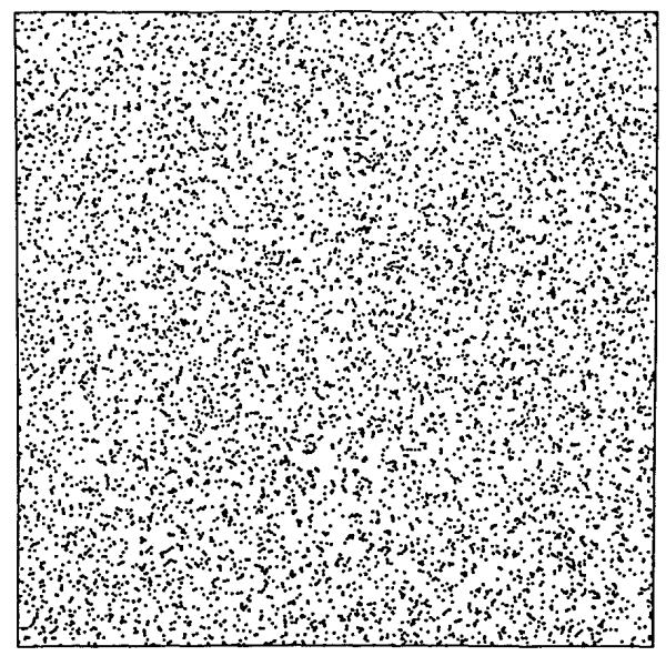
Array of points generated by a uniform random number generator. What is the variation in the density of points?

The value of the mean is known, 8,192 points per unit square. To measure the variation in local point density we might overlay grids with differently sized pixels, as in Fig. 2. The RD for the number of points for the 4-pixel grid was 2.2010, for the 16-pixel grid was 4.6%, and for the 64-pixel grid was 8.9%. This was extended to finer grids. The plot of the logarithm of RD vs. the logarithm of the number of pixels is shown in Fig. 3. The expected slope is that with each quadrupling of the number of pixels the RD should increase by a factor of two. Fitting a linear regression to the logarithms (admitting that this may not be a completely appropriate regression in view of the fact that the original data were in a linear, not logarithmic, domain as critiqued by Berkson (4)), gave an estimated slope of 0.4965. The fractal, or power law, expression is:

$$\frac{\mathit{RD}\left(n\right)}{\mathit{RD}\left(64\right)}={\left(\frac{n}{64}\right)}^{0.4965},$$ (3)

where N = 64 was the arbitrarily chosen reference number of pixels. The estimated fractal D was 1.4965 compared to the theoretical value of 1.5.

FIGURE 2.

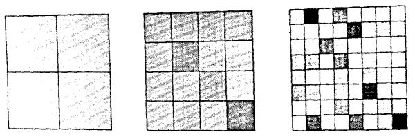
Overlay of grids with differing mesh sizes on the array of uniform random points in Fig. 1. The gray shade assigned to each pixel indicates the % difference between the number of points in the pixel and the mean number of points per pixel at that pixel size. White indicates 20% below the mean and black 20% above the mean.

FIGURE 3.

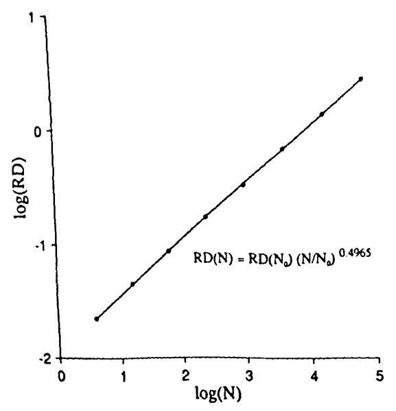
Relative dispersions obtained from the uniform random points of Fig. 1 as a function of the number of pixels (N) in the grid. The slope of the regression line is close to the theoretical value of 0.5.

RESULTS WITH NONRANDOM ARRAYS

Performing the same exercise with nonrandom arrays leads to an interesting result. Correlation between the local densities of neighbors was obtained by generating a function whose densities, while still probabilistic, were distinctly shaped over the field. Gaussian, 2-dimensional profiles resulted from generating the sum of two sets of points, each from a random number generator producing a Gaussian density function with standard deviation of 0.15, centered at (X, Y) = (0.3,0.3) and (0.7,0.7). The number of point totaled 8,192, as in Fig. 1, so that the mean densities are identical in Figs. 1 and 4. The same sequence of grids was placed over this correlated array, and RD calculated for each mesh size as before. The results, shown in Fig. 5, differ in two respects: the line is no longer a simple power law relationship and, at mesh sizes below 64 × 64 pixels, the slope of the line of RD vs. mesh size is less than for uniformly distributed data.

FIGURE 4.

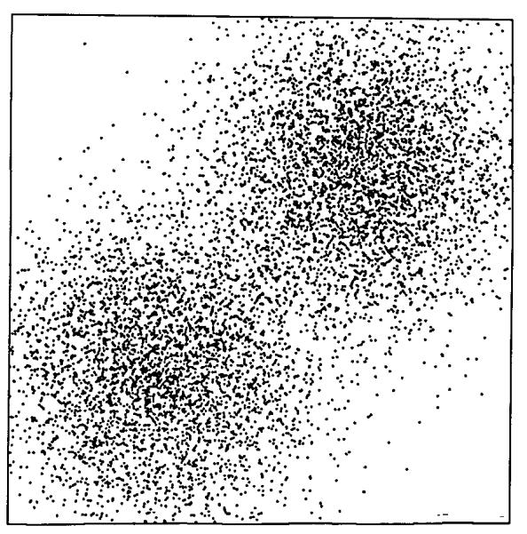
Array of points generated from the sum of two Gaussian distributions (SD = 0.15) centered at X, Y = 0.3,0.3 and 0.7,0.7. The total number of points is 8192.

FIGURE 5.

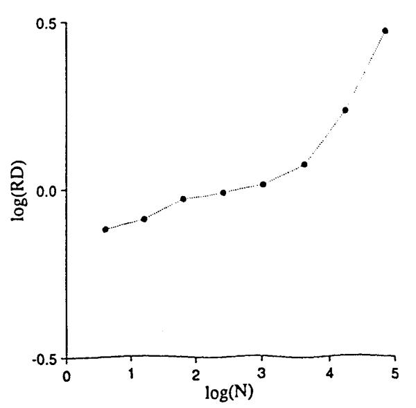
Relative dispersions for different mesh sizes on the array of Fig. 4.

AN EXPLORATION OF CONTINUOUS DISTRIBUTIONS

Instead of generating the positions of points with a statistical distribution of locations in 2-space, we generated the continuous distribution shown in Fig. 6. It has the same mean probability densities, or concentrations, as for Fig. 4. The mesh was 64 × 64 (2⁶ by 2⁶) for a total of 4,096 (2¹²) squares within the original unit square. Within each pixel the concentration was considered uniform. The grids were overlaid, the average concentration calculated for each grid unit, and the RDs calculated for the field as before. The result is trikingly different. The relationship between RD and the number of grid elements, shown in Fig. 7, now has a clearly defined plateau beyond which further refinement of the grid element size, or resolution of the observation element size, gives no further increase in the observed heterogeneity. The plateau begins at the grid resolution that matches the pixel size of the original continuous distribution. The result is inevitable, namely that subdividing internally uniform units produces no increase in the apparent dispersion of the concentrations.

FIGURE 6.

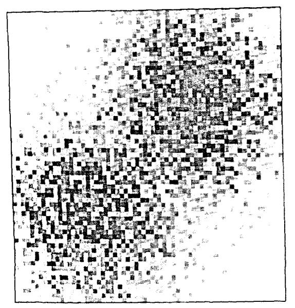
Continuous representation of the Gaussian distributions shown in Fig. 4. Each of the 4096 pixels is internally uniform in concentration.

FIGURE 7.

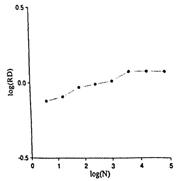
Relative dispersions for different mesh sizes on the continuous distribution of Fig. 6.

CONTINUOUS DISTRIBUTIONS WITH SUBUNITS CONTAINING NEGATIVELY CORRELATED SUBUNITS

In dichotomous branching systems where a parent source divides into two daughter branches, there is an opportunity for negative correlation between the daughter branches. An example is the twinkling of local flows in the microvasculature where, if the flow in the parent source is held constant but that in one daughter branch increases, then the flow in the other daughter branch must decrease. We examined a simple case of this type.

Each of the pixels of Fig. 6 was further subdivided using the pattern of 16 subunits on a square grid (Fig. 8) where the concentrations in the dark squares were set to be one eighth the mean concentration of the original, and those in the light squares were set to zero. Thus, the mean number of points in the unit square remained unchanged at 8,192. Again the RDs were calculated for the various grids.

FIGURE 8.

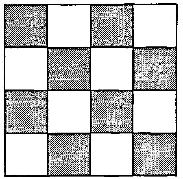
Checkerboard pattern used for further subdividing each of the 4096 pixels in Fig. 6.

The results, shown in Fig. 9, are identical to those in Fig. 5 up through the division into 4,096 units, log (N) = 3.6. The next division into 16,384 units produces no increase in observed dispersion since each of the four quarters of Fig. 8 has the same mean as the whole square. The next division, however, shows a sudden increase in observed dispersion since the heterogeneity of the units is now revealed. As in Fig. 7, further division of these now uniform units does not increase the observed dispersion beyond the second plateau.

FIGURE 9.

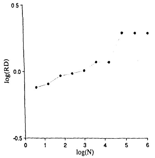
Relative dispersions for different mesh sizes when there is negative correlation within the 4096 units as in Fig. 8.

The negative correlation produces a segment of the slope of log RD vs. log (N that has a slope with a fractal dimension greater than 1.5, that is, with a fractal D greater than that of random noise. Since such possibilities for negative correlation exist in many biological situations, combinations of positively and negatively correlated features in tissue structures or functions should not be thought of as strange.

ESTIMATES OF HETEROGENEITY OF REGIONAL MYOCARDIAL BLOOD FLOWS

We reconstructed sheep hearts that had been divided into about 250 identified pieces into aggregates composed of nearest neighbors. Given these data, we could numerically divide the heart into 4, 8, 16, etc. sections, each composed of pieces that were originally neighbors (see Fig. 10). Division of the left ventricle into four regions in each of 11 hearts resulted in the highest peak distribution in Fig. 10; division into 192 pieces of average mass O.22g gave the broadest, lowest peaked distribution. Figure 11 shows the results when the log of the RD is plotted against the log of the average piece size. (This is equivalent to Fig. 3, realizing that decreasing piece mass is equivalent to increasing the number of pixels). The low end of the range of piece size is limited by the resolution with which the heart was originally divided, i.e. about 220 mg. The data from 10 baboon and 11 sheep hearts can be summarized by the equation:

$$\mathit{RD}\left(m\right)=18\cdot m^{-0.2}(D=1.2)$$ (4)

FIGURE 10.

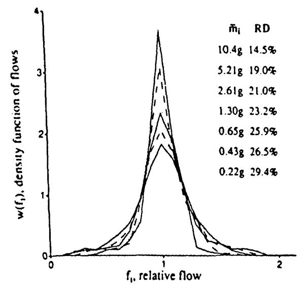
The effect of sample size on the apparent dispersion of regional myocardial blood flow in the left ventricle of 11 sheep hearts. Data were obtained using the “molecular microsphere” iododesmethylimipramine. The average mass of the pieces. m_i, are in the order of the peak heights of the distributions and the RDs increase with finer divisions. [Reprinted from Bassingthwaighte et al. (3) by permission of the American Heart Association. Inc.]

FIGURE 11.

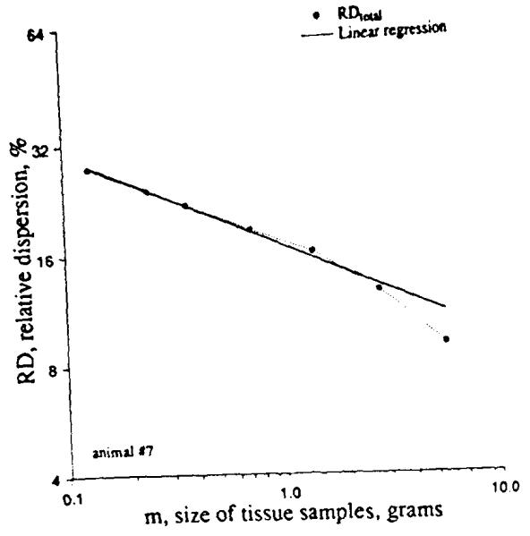
Fractal relationship between the relative dispersions of regional flows (measured by the deposition of microspheres in the heart of a baboon) and the average mass of the pieces into which the heart was divided. The equation of the regression line is RD(m)=16.9m^−0.25 (r=0.996) The rightmost point was not used in the regression. [Reprinted from Basslngthwalghte and van Beek (2). Copyright 1988 IEEE.]

SPATIAL CORRELATION IS CHARACTERIZED BY THE FRACTAL DIMENSION

An intriguing and useful feature of the fractal relationship is that it specifies the degree of correlation between neighbors in a spatial domain. In the preceding section, we considered the relative dispersion, or coefficient of variation, of regional flows as a one-dimensional intensity, analogous to a voltage as a function of time. It is better to consider regional flow as the intensity of a property of the myocardium in three-dimensional space, just as we would consider the water density in a cloud at different positions in a three-dimensional domain. In reconstructing the heart from the smallest pieces cut into larger and larger pieces, we were careful always to group together the nearest neighbors to form the aggregates of a larger size. When pieces of a given size are cut in half, then the increase in apparent variation will be greater when the two halves of each piece are uncorrelated than when they are correlated. Van Beek worked out a general relationship (11) for the correlation coefficient, r = 2^3−2D − 1.

When D = 1.5, then r = 0, and when D = 1.0, r = 1, fulfilling expectations. With D = 1.2, the average for our sheep and baboon hearts, then r = 2^0.6 − 1 = 1.6 − 1 = 0.6, or 60%. This is the correlation between nearest neighbor voxels (volume elements) of equal volume. Because the system has statistically fractal self-similar properties there is the same degree of correlation between adjacent 1-mm cubes as between adjacent l-cm cubes. The correlation between voxels that are not adjacent is less; the correlation between pieces of any particular size falls off monotomcally but not exponentially.

CAN WE PREDICT THE SIZE OF THE MYOCARDIAL MICROVASCULAR UNIT?

The fractal slopes differed from animal to animal, but in each set of observations it was consistent that those animals that exhibited large relative dispersion at any chosen reference size had lower fractal dimensions, slopes, than did those that had small relative dispersions at that chosen size. Preliminary evidence for a given species suggests that the family of lines might intersect at a common point. This idea was applied by Roger et al. (7) as illustrated for the sheep data in Fig. 12.

FIGURE 12.

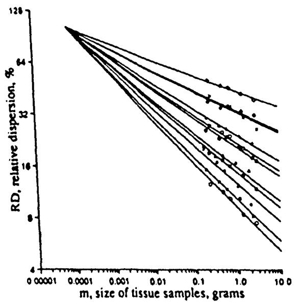
Projection of the fractal relationships for the relative dispersions of regional myocardial flows in 11 sheep through a common point. The best fit was obtained with m = 75 μg and RD = 102% (r = 0.975).

The point of intersection is at RD = 102% at a volume element size of 75 μg. This intersection suggests that 75 μg is the size of a microvascular unit. This would suggest that these are 13 arterioles per mm³ of tissue, in line with estimates made by others (5,6,1). But an RD of 102% is large compared to the 50% RD seen in hamster hearts (10) using quantitative autoradiography with element sizes less than 100-cubic microns, using the “molecular microsphere” iododesmethylimipramine. For the sheep and baboons data, the 102% RD was an extrapolation from the smallest observed pieces of about 100 mg down to pieces of less than 100 μg, three orders of magnitude smaller.

Was the extrapolation simply over too large a range or is the heterogeneity less in small hearts? Van Beek et al. (11) sought to resolve this apparent disparity by developing a dichotomously branching model of the arterial system that has the appropriate relative dispersions. The heterogeneity was given by asymmetry in flow at each branch point; 3% to 4% deviation from 50% sufficed. The branching network has fractal characteristics, the division of flow being self-similar on scaling. This does not result in straight log–log plots as in Fig. 11, but rather in convex-upward curves that gave a common intersection at a much lower RD, 55%, close to that of the hamsters. Analysis of autoradiographic resolution data on the larger hearts is now required to determine if their flow heterogeneity is fundamentally different than that of the smaller hamster hearts.

It may be reasonable that the heterogeneity in larger hearts is greater at a given unit size than in small hearts. Since there must be a larger number of generations of branching to supply a given unit size in a large heart than in a small one.

CONCLUSION

Fractals are useful tools for examining flow heterogeneity. First, they describe flow heterogeneity over a large range of sizes of the observed tissue samples. Second, fractally branching arterial networks can explain such observed heterogeneity. Third, they predict the functional microvascular unit size. Since appropriate data have not been obtained, the extrapolation is too great to instill confidence, but it is testable by experiment.

Fractal geometry is not proven to be the basis of flow heterogeneity in the myocardium, but the use of fractal approaches provokes questions that push one to investigate more deeply.

REFERENCES

- 1.Bassingthwaighte JB, Yipintsoi T, Harvey RB. Microvasculature of the dog left ventricular myocardium. Microvasc. Res. 1974;7:229–249. doi: 10.1016/0026-2862(74)90008-9. [DOI] [PMC free article] [PubMed] [Google Scholar]
- 2.Bassingthwaighte JB, van Beek JHGM. Lightning and the heart: Fractal behavior in cardiac function. Proc. IEEE. 1988;76:693–699. doi: 10.1109/5.4458. [DOI] [PMC free article] [PubMed] [Google Scholar]
- 3.Bassingthwaighte JB, King RB, Roger SA. Fractal nature of regional myocardial blood flow heterogeneity. Circ. Res. 1989;65:578–590. doi: 10.1161/01.res.65.3.578. [DOI] [PMC free article] [PubMed] [Google Scholar]
- 4.Berkson J. Are there two regressions? J. Am. Stat. Assoc. 1950;45:164–180. [Google Scholar]
- 5.Eng C, Cho S, Factor SM, Sonnenblick EH, Kirk ES. Myocardial micronecrosis produced by microsphere embolization: Role of an α-adrenergic tonic influence on the coronary microcirculation. Circ. Res. 1984;54:74–82. doi: 10.1161/01.res.54.1.74. [DOI] [PubMed] [Google Scholar]
- 6.Kaneko N. The basic structure of intramyocardial microcirculation system in the normal human heart. In: Tsuchiya J, Asano M, Mishima Y, Oda M, editors. Microcirculation - an update. Vol. 2. Amsterdam; Elsevier Science Publishers: 1987. pp. 159–160. [Google Scholar]
- 7.Roger SA, van Beek JHGM, Bassingthwaighte JB. Estimating the functional myocardial microvascular unit size using fractal models. Microvasc Res. (under review) [Google Scholar]
- 8.Rogers A. Statistical Analysis of Spatial Dispersion. Pion; London, England: 1974. [Google Scholar]
- 9.Snedecor GW, Cochran WG. Statistical Methods. Iowa State University Press; Ames, IA: 1980. [Google Scholar]
- 10.Stapleton D, van Beek J, Roger SA, Baskin DG, Bassingthwaighte JB. Regional myocardial flow heterogeneity assessed with 2-iododesmethylimipramine. Circulation. 1988;78:II 405. [Google Scholar]
- 11.van Beek JHGM, Roger SA, Bassingthwaighte JB. Regional myocardial flow heterogeneity explained with fractal networks. Am. J. Physiol(Heart.Circ.PhysioI.26) 1989;257:H1670–H1680. doi: 10.1152/ajpheart.1989.257.5.H1670. [DOI] [PMC free article] [PubMed] [Google Scholar]