SENSOP: A Derivative-Free Solver for Nonlinear Least Squares with Sensitivity Scaling

Abstract

Nonlinear least squares optimization is used most often in fitting a complex model to a set of data. An ordinary nonlinear least squares optimizer assumes a constant variance for all the data points. This paper presents SENSOP, a weighted nonlinear least squares optimizer, which is designed for fitting a model to a set of data where the variance may or may not be constant. It uses a variant of the Levenberg–Marquardt method to calculate the direction and the length of the step change in the parameter vector. The method for estimating appropriate weighting functions applies generally to 1-dimensional signals and can be used for higher dimensional signals. Sets of multiple tracer outflow dilution curves present special problems because the data encompass three to four orders of magnitude; a fractional power function provides appropriate weighting giving success in parameter estimation despite the wide range.

INTRODUCTION

The weighted nonlinear least squares problem arises from the need to fit curves and estimate parameters. One attempts to fit a set of data (with inhomogeneous variance) with a mathematical model where the parameters appear nonlinearly. The weighted nonlinear least squares problem consists of choosing parameters so that the fit is as close as possible. Data are necessarily noisy, but the noise effects are offset by using a larger number of data points than the number of free parameters. Weighted nonlinear least squares methods, which minimize the sum of squares of weighted deviations, are a variant of the ordinary nonlinear least squares, which minimizes the sum of squares of unweighted or evenly weighted deviations.

An ordinary least squares model fitting criterion yields efficient parameter estimates if the errors are random, are uncorrelated and have common mean zero. The errors should also have constant variance independent of position within the data set. In fitting multiple tracer outflow dilution curves and residue data, the variances for the individual data points are not constant. For example, the data of Kroll et al. (10) for a multiple tracer study using albumin, l-glucose, and uric acid encompass a 4 order of magnitude range; the absolute variance is greater at the peaks of the curves (of the type shown below in Fig. 3) but the relative error is much less than those at very early or late time points; certain parameters of models are highly dependent on the waveform at the peaks of the curves, while others are wholly determined from the tails, so the whole range is important. Box and Hill (4) suggested using a power transformation and combining with ordinary least squares to tackle the problem of inhomogeneous variances. The use of nonlinear least squares is very computationally intensive, in part because the method of power transformation has to use the nonlinear least squares solver several times in order to determine the appropriate power. In this case, the weighted least squares solver is more efficient if the weights can be obtained directly.

FIGURE 3.

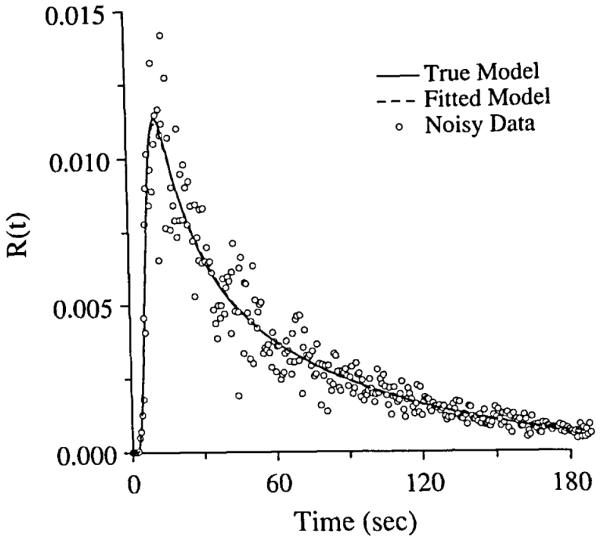
Fitting of blood–tissue exchange model, BTEX30, to simulated residue function data with 20% Gaussian Noise. The open circles were the noise added residue curve. The solid line curve was the model solution with the exact parameters. The dashed line curve was the model solution with the fitted parameters, and almost exactly matches the curve with the exact parameters.

There are available a number of programmed routines that solve ordinary nonlinear least squares problems. An evaluation of these “state of the art” mathematical software routines was given by Hiebert (9). We present herein SENSOP, a routine that is general, but that works particularly well for fitting data covering a wide range, such as tracer dilution data to be fitted with our blood-tissue exchange model (2).

SENSOP was developed to handle problems of parameter determination from multiple sources of data. Because complex models may be used to fit thousands of data sets, efficiency in finding a solution is critical. All too often it is difficult to differentiate such model functions analytically, so constructing a subroutine for the computation of the Jacobian is not only time consuming but also introduces another source of error. SENSOP, for simplicity of code and usage, uses numerical differentiation. Even though the numerical differentiation will lead to less accurate results than using analytical differentiation, an optimal or nearly optimal mesh spacing will increase the accuracy of the numerical differentiation.

THE THEORY OF THE SENSOP OPTIMIZATION METHOD

Since the notation used in the field of curve fitting and parameter optimization is so varied, the notation used in this paper is defined next.

Notation

The observed data y_i, i = 1, … , m are described by the following equations:

$$y_i=f(\theta ,x_i)+r_i\text{for}i=1,\dots ,m,$$ (1)

where f(θ,x_i) is a mathematical model, a function of the parameter vector θ of dimension p, x_i is the independent variable defined at m points, and the r_i are random errors with mean zero and variance ${\sigma }_i^2$. In vector notation:

$$Y=F(\theta ,X)+R.$$ (2)

We denote an m × m weighting matrix by

$$W=\mathrm{diag}(w_1,w_2,\dots ,w_m),$$ (3)

where $w_i=1∕{\sigma }_i^2$.

Let the m × 1 residual vector be given by

$$R\left(\theta \right)=Y-F(\theta ,X).$$ (4)

Let the sum of squares of weighted residuals SSR(θ) be denoted by

$$\mathrm{SSR}\left(\theta \right)=\frac{1}{2}\sum _{i=1}^m{(f(\theta ,x_i)-y_i)}^2{w}_i=\frac{1}{2}R{\left(\theta \right)}^{T}WR\left(\theta \right).$$ (5)

The Jacobian matrix is defined as ∂f(θ,x)/∂θ in its continuous form, but requires redefinition where numerical derivatives requires taking a finite step in θ. Therefore, the sensitivity matrix S(θ) is defined with components

$$s({\theta }_j,x_i,h_{ij})=\frac{f(\theta +h_{ij}{I}_j,x_i)-f(\theta ,x_i)}{h_{ij}}\text{for}1\le i\le m\text{and}1\le j\le p,$$ (6)

and is an approximation of the Jacobian matrix, where I_j is the jth column of a p × p identity matrix, and h_ij is the step size or mesh spacing for jth parameter and ith observation.

Mesh Spacing

In the numerical approximation of derivatives by finite differences there are two types of errors, both step-size dependent: one varies with 1/h_ij and the other with h_ij. The error in the partial derivative of f(θ,x_i) with respect to the jth component of θ is weighted by |1/h_ij|, at the ith observation. The truncation error of the numerical estimate of the derivative is weighted by |h_ij|. Two different methods may be used for selecting a value of h_ij to compromise this opposition:

1. Minimize the sum of the worst error magnitudes.

2. Use the “folk-dictum” as in Eq. 9: choose h_ij so that the significance of function differences is halved.

Specifically by the first method we mean: find a|h_ij| to minimize the bound B_ij, where

$$B_{ij}=2{\zeta }_{i}f(\theta ,x_i)∕\mid h_{ij}\mid +0.5M\mid h_{ij}\mid .$$ (7)

Here M is an upper bound for the second derivative |∂²f(θ,x)/∂θ²|, and ζ_if(θ,x_i) is an upper bound for the “noise” on f(θ,x_i). Then

$$\mid (f(\theta +h_{ij}{I}_j,x_i)-f(\theta ,x_i))∕h_{ij}-f^{\prime }(\theta ,x_i)\mid \le B_{ij}.$$ (8)

By the second method we mean choosing h_ij such that

$$\mid f(\theta +h_{ij}{I}_j,x_i)-f(\theta ,x_i)\mid =\sqrt{{\zeta }_i}\mid f(\theta ,x_i)\mid ,\text{for}j=1,\dots ,p.$$ (9)

Both of the above principles will be utilized. We do not, however, wish to spend the time required to adjust m ×p different step sizes |h_ij| that the above principles seem to require. We shall reduce this number to p as illustrated in the next section.

Updating the Parameter Vector and Mesh Spacing

The following variant of the Levenberg–Marquardt method (13,14) will be used to find an approximate solution vector θ, which minimizes the SSR(θ).

$${\theta }^{k+1}={\theta }^k-\gamma {(S{\left({\theta }^k\right)}^{T}WS\left({\theta }^k\right)+\alpha I)}^{-1}\times S{\left({\theta }^k\right)}^{T}WR\left({\theta }^k\right),$$ (10)

where α = β∥S(θ^k)^TWR(θ^k)∥₂ and β is a positive constant, I is the p × p identity matrix, γ ≤ 1 is a relaxation coefficient, which we called the Levenberg–Marquardt or L–M coefficient, and k is the index of iteration.

We now indicate how the folk-dictum of Eq. 9 is implemented. The initial spacing is calculated from the upper bound for the noise, being given by $h_{ij}^0=\sqrt{{\zeta }_i}{\theta }_j$, 1 ≤ j ≤ p, 1 ≤ i ≤ m, if θ_j ≠ 0; otherwise $h_{ij}^0=\sqrt{{\zeta }_i}$. New spacings will be updated by the formula

$$\mid h_{ij}^{k+1}\mid =\frac{\sqrt{{\zeta }_i}\mid f({\theta }_j,x_i)\mid }{\mid s({\theta }_j,x_i,h_{ij}^k)\mid },$$ (11)

where $({\theta }_j,x_i,h_{ij}^k)$ is the component of the sensitivity matrix at the kth iteration. Equation 11 is obtained by linearization of f(θ + h_jjI_j,x_i) using $s({\theta }_j,x_i,h_{ij}^k)$ and invoking Eq. 9. While this formula could be used to generate a sequence of hopefully improved updates, we shall only update with it once for each index k.

To avoid computing the mesh spacing for each i, 1 ≤ i ≤ m we shall do “sensitivity scaling.” To compute the step length for the jth column of the finite difference approximation of the Jacobian or sensitivity matrix, an index q that maximizes |s(θ_j,x_i,h_ij)| over 1 ≤ i ≤ m is chosen. Then $h_{qj}^{k+1}$ is computed from Eq. 11 above. These spacings $h_{qj}^{k+1}$ are used to calculate the approximate Jacobian for the next iteration. Since the sensitivities are more or less smooth, the selection of the qth point represents choosing a region of the sensitivity function; using the center index of a region is an alternative approach. This process increases the accuracy of certain entries in the columns of the Jacobian: namely, those entries where the model function is most sensitive to the parameter associated with that column. Since the index q is a constant for each jth parameter and each kth iteration, from now on we will drop the index q when we refer the step size $h_{qj}^k$, i.e., $h_{qj}^k=h_j^k$.

It remains to discuss the use of the bound B_ij in Eq. 7. Because Eq. 7 requires estimation of second derivatives, it would be wasteful of function evaluations to use it too often. When the algorithm below terminates, an extra step can be made using Eq. 7 in the same way that Eq. 9 would have been applied. Generally, the result is more accurate than would have been obtained by Eq. 9.

IMPLEMENTATION OF THE SENSOP ALGORITHM

The algorithm can be described generally:

• 0)Estimate the weighting function w_i, from the local variances, ${\sigma }_i^2$, for i = 1, … , m.
• 1)Set k = 0, define the initial parameter vector θ⁰ and the initial step size $h_j^0$.
• 2)Compute the $w_i^{1∕2}$ for i = 1, … , m and store the result.
• 3)Compute the model function f(θ,x_i), for i = l, … , m.
• 4)Compute the weighted deviation $r(\theta ,x_i)w_i^{1∕2}=(y_i-f(\theta ,x_i))w_i^{1∕2}$ for i = 1, … , m.
• 5)Compute the sum of squares of weighted deviation SSR(θ^k).
• 6)Compute the matrix S(θ^k).
• 7)Select the sensitive data points, which have the largest absolute values of the sensitivity function values, and update the step size for each parameter, h_j.
• 8)Compute the L–M coefficient α, for Eq. 10.
• 9)
  Solve the linear equations for the step increment in the parameter vector,

  $$\Delta \theta ={(S{\left({\theta }^k\right)}^{T}WS\left({\theta }^k\right)+\alpha I)}^{-1}S{\left({\theta }^k\right)}^{T}WR\left({\theta }^k\right).$$ (12)
• 10)Find the modified step length γ for Eq. 10 by halving the step increment until SSR(θ^k − γΔθ) ≤ SSR(θ^k).
• 11)Update the solution θ^k+1 = θ^k − γΔθ.
• 12)
  Check if any of the following criteria are met:

  1. The number of function generations exceeds a maximum number.
  2. The sum of squares of weighted deviations, SSR(θ) from Eq. 5, is less than a preassigned level.
  3. The size of gradient of sum of squares of weighted deviation ∥S(θ^k)^TWR(θ^k)∥ is less than a pre-assigned tolerance.
  4. The relative step change in the parameter vector is smaller than a chosen value. The calculation of the relative step size is

     $${\left(\sum _{j=1}^p{\left(\frac{\Delta {\theta }_i}{\mathrm{MAX}(\mid {\theta }_i\mid ,∊)}\right)}^2\right)}^{1∕2},$$ (13)

     where ε is a small positive number representing a machine precision.
  5. If none of the stopping criteria is met, k = k + 1, go to Step 3.
  6. When a stopping criterion is met, compute the confidence interval for parameters, and terminate the algorithm.

METHODS OF ESTIMATING THE WEIGHTING FUNCTION

There are many ways to estimate a weighting function, with the optimal weighting function being the inverse of the variance of the data point $(w_i=1∕{\sigma }_i^2)$, (16). One may of course obtain an unweighted (evenly weighted) fit of the model to the data, or any other personally chosen weighting scheme. For a general approach, the variances of data points were obtained by using the fitted deviations of n_n nearest neighboring points,

$${\widehat{\sigma }}_i^2=\frac{1}{n_n}\sum _{k=i-n_n∕2}^{k=i+n_n∕2}{(y_k-f(\theta ,x_k))}^2.$$ (14)

The unweighted fit is biased when the variances for individual data points differ; the estimates of weighting function may be inappropriate. Several iterations of the process (which uses the estimated weighting function to estimate yet another weighting function by a weighted fitting) can be used to negate the biases in estimating the variance of the data points.

The repetition of nonlinear fitting is computationally intensive, one may replace the model fitting by fitting piecewise polynomials to the data. To obtain a piecewise polynomial, we minimize

$$\sum _{j=1}^J\sum _{k=1}^{n_j}{(P_j\left(x_{n_1+n_2+\dots +n_{j-1}+k}\right)-y_{n_1+n_2+\dots +n_{j-1}+k})}^2,$$ (15)

where J is the number of partitions of data points, and n_j the number of observations in the jth partition.

Using the residuals of the fit, we can estimate the error variance of y_i. We use a moving average with n_m + 1 fitting deviations, i.e.,

$${\widehat{\sigma }}_i^2=\frac{1}{n_m}\sum _{u=i-n_m∕2}^{i+n_m∕2}{(P_j\left(x_u\right)-y_u)}^2.$$ (16)

The weighting function $w_i=1∕{\widehat{\sigma }}_i^2$ (16) obtained here is not dependent upon a single point, i.e., the estimation will be stable in the presence of noise.

For multitracer outflow experiment data such as that of Kroll et al. (10), we used a weighting function which is in inverse proportion to a power function of the datum point

$$w_i=\frac{1}{y_i^{\psi }},$$ (17)

where ψ is a positive constant in the range from 0 to 1. This is in accord with the idea that noise in the measurement of tracer activity is proportional to the reciprocal of the number of counts, modified by pipetting error, etc. We commonly used ψ = 0.56. For a positive datum value, y_i, when ψ = 0, the weighting function is a constant one, and the fitting is equivalent to the fitting of ordinary least squares. When ψ = 1, the fitting is equivalent to the fitting in a logarithmic domain. Using ψ in the middle, 0.5–0.6, gives a compromise, a “best fit” over the three orders of magnitude of the data when there are relatively more low values than high values. If the range is greater or the number of low points is smaller, then a larger ψ is used to achieve a balanced weighting.

CONFIDENCE INTERVALS OF ESTIMATED PARAMETERS

The covariance matrix of the solution parameters can be estimated by the Hessian matrix at the solution (i.e., the second derivative matrix). Near the solution for small residuals, the right hand side of Eq. 18 below is an approximation to the covariance matrix,

$$\mathit{Cov}\left(\theta \right)=\left(\frac{\mathrm{SSR}\left(\theta \right)}{m-p}\right){\left(S{\left(\theta \right)}^{T}WS\left(\theta \right)\right)}^{-1}.$$ (18)

Based on the approximation, the 95% confidence interval for the parameter θ_j, will be

$${\theta }_j\pm t_{m-p,0.95}\sqrt{\mathrm{diag}{\left(\mathit{Cov}\left(\theta \right)\right)}_j},$$ (19)

where t_m–p,0.95 is the Student’s t-distribution with m – p degrees of freedom (17).

The estimates of the confidence interval will be underestimated if the model function f(θ,x_i) is highly nonlinear and the residuals are large. We choose this linearization method of calculation for the covariance matrix, because the major part of calculation S(θ)^TWS(θ) is already done in the optimization process. To measure the goodness of estimated confidence interval, one may perform a simulation study by repeated trials on fitting model solutions to data to which the experimentally appropriate levels of random noise have been added. If high accuracy of the confidence interval is desired, one may try a more computationally intensive method such as that of Duncan (8) in which asymmetry of the upper and lower limits is properly treated. An extensive comparison of various methods for the confidence intervals was reported by Donaldson and Schnabel (7).

NUMERICAL RESULTS

SENSOP was tested on a variety of examples and practical problems, and its behavior compared to several time-tested curve fitting algorithms. The problem sets include test problems listed in Moré, Garbow, and Hillstrom (15), and the practical problems of fitting tracer data with blood-tissue exchange models (2). The curve fitting routines tested against SENSOP were the IMSL (International Mathematical and Statistical Library, Houston, TX) routine ZXSSQ, and the TOMS algorithm 573, NL2SNO [the derivative-free version of NL2SOL, which solves the nonlinear least squares problem, written by David M. Gay (6)].

Weighted Versus Unweighted

In order to compare the results of the weighted nonlinear least squares optimizer and ordinary nonlinear least squares, we chose SENSOP (the weighted least squares solver) and ZXSSQ (an IMSL routine for nonlinear least squares). Both of the routines use the Levenberg–Marquardt step calculations. The data used to compare the parameter estimates for both methods were generated by using a modified Gaussian function (15) with 50% uniform random noise added,

$$y_i=0.4e^{-0.5{\left(x_i\right)}^2}\times (1\pm 0.5\times U[0,1])\text{for}i=1,\dots ,15,$$ (20)

where x_i = (8 — i)/2. The model function used to fit the data is a Gaussian type function (15), i.e.,

$$f(\theta ,x_i)={\theta }_1{e}^{-0.5{\theta }_2{(x_i-{\theta }_3)}^2}.$$ (21)

The correct values should therefore be θ₁ = 0.4, θ₂ = 1.0, and θ₃ = 0; however, only a single realization of the noisy functions was fitted, which means that the noise-free function cannot be identified by any method. The following are the results generated by SENSOP and ZXSSQ using single precision arithmetic with five different sets of starting values. Only the relative step size was used as a stopping criterion, the routines terminated when the L-2 norm of the relative parameter changes was less than 10⁻⁴.

The parameter estimates using weighted least squares are better in the sense that they are closer to the true values than those of unweighted least squares. Since only one data set was used for the trials in Tables 1 and 2, the systematic deviations in the final estimates presumably reflect the form of the particular data set. In this problem, the expected variance of y_i is equal to f(θ,x_i)/12, i.e., the variance is inhomogeneous across the whole set of the data. In Fig. 1, the curves fitted via ZXSSQ (unweighted fit) and SENSOP (weighted fit) were plotted along with the true underlying model (curve with the solid line type) and its noisy representation (curve with the open circle symbols). Note that the ZXSSQ fit (curve with the dashed line type) appears systematically narrower. Using SENSOP with uniform weighting (unweighted) gave essentially similar estimates to those obtained with ZXSSQ.

TABLE 1. Results of weighted fitting on Gaussian function.

	Final Parameter Estimates
Starting Value	θ 1	θ 2	θ 3
(0.4, 1, 0)	0.4060	1.0861	0.0514
(0, 0, 0)	0.4060	1.0862	0.0512
(0.5, 0.5, 0.5)	0.4060	1.0861	0.0514
1, 1, 1	0.4060	1.0861	0.0514
(2, 2, 2)	0.4060	1.0861	0.0514

TABLE 2. Results of unweighted fitting on Gaussian function.

	Final Parameter Estimates
Starting Value	θ 1	θ 2	θ 3
(0.4, 1, 0)	0.4547	1.1952	0.1198
(0, 0, 0)	0.4547	1.1951	0.1198
(1, 1, 1)	0.4547	1.1951	0.1198
(0.5, 0.5, 0.5)	0.4547	1.1953	0.1198
(2, 2, 2)	0.4547	1.1952	0.1198

FIGURE 1.

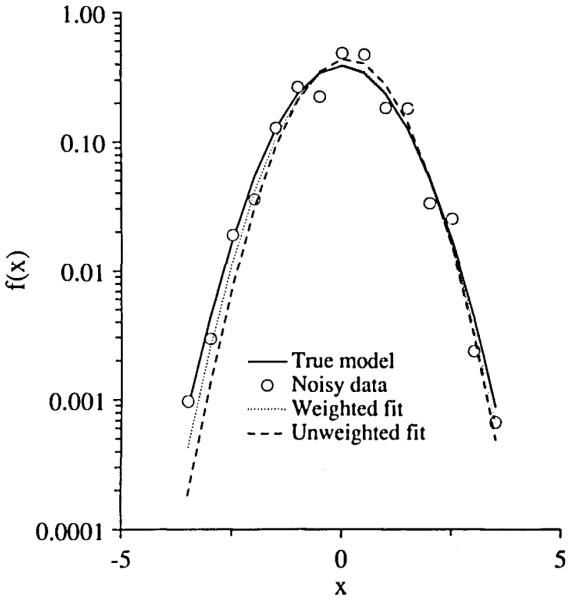
The generated data with 50% uniform random noise added to Gaussian function (○). The curve with solid line was the true Gaussian function. The data were fitted by weighted least squares routine SENSOP (····) and unweighted least squares routine ZXSSQ (---).

Multi-Exponential Curve Fitting

Biggs 6EXP (15) was used to compare the derivative-free methods of nonlinear least squares, ZXSSQ and NL2SNO and nonlinear least squares with sensitivity scaling, SENSOP. NL2SNO uses quasi-Newton step calculation. The ψ of the weighting function in SENSOP, Eq. 17, was set to 0.0, which is equivalent to solving an ordinary least squares problem.

The Biggs 6EXP model functions are

$$f(\theta ,x_i)={\theta }_1{e}^{-x_i{\theta }_2}-{\theta }_3{e}^{-x_i{\theta }_4}+{\theta }_5{e}^{-x_i{\theta }_6},$$ (22)

where x_i = 0.1 × i, i = 1, … ,30. The data functions

$$y_i=e^{-x_i}-5e^{-10x_i}+3e^{-4x_i},$$ (23)

with minimal sum of square residuals zero at (1,1,5,10,3,4), i.e., this is a no-noise case. These particular values are chosen because they pose a difficult optimization problem even in the absence of noise and even though the function covers only a twenty fold range of values.

The problem of fitting multi-exponential functions is well known to be difficult computationally. The extreme sensitivity of the exponent was pointed out by Lanczos (12), who showed for a particular example that various parameter values can give near-optimal results. Fitting a multi-exponential function to time course data is widely used for obtaining estimates of kinetic parameters. An example is the fitting of tracer washout data with Eq. 22 representing a three-compartmental system.

The following tables summarize the results generated by single precision versions of SENSOP, ZXSSQ and NL2SNO with five different sets of starting values: (1, 1, 1, 2, 1, 1), (1, 1, 1, 20, 1, 1), (5, 5, 5, 5, 5, 5), (10, 10, 10, 10, 10, 10) and (1, 1, 1, 10, 1, 1). The runs were performed on the Cray 2 at San Diego Supercomputer Center. No vectorization of the code was done to speed up SENSOP or NL2SNO. We used the library routine ZXSSQ, LINPACK routines and BLAS routines installed on the Cray 2 machine, for which some improvements by vectorization had been achieved.

We used the relative parameter change and the sum of squares of residuals as the stopping criteria for these routines; the algorithms stopped when the L-2 norm of the relative parameter changes (Eq. 13) was less then 10⁻⁶ and the sum of squares of residuals was less than 10⁻¹⁰. Figure 2 shows the parameter vectors as functions of the number of iterations for SENSOP (Fig. 2a) and for NL2SNO (Fig. 2b). There are plotted the normalized parameter vectors generated by SENSOP with a starting parameter vector (1, 1, 1, 2, 1, 1). At the 11th iteration, the solution obtained by SENSOP was within 0.1% accuracy. It took 14 iterations to achieve the 0.0001% accuracy. For fitting our dilution outflow curve, we are satisfied with 1% accuracy. For the five trials with the different starting values, on the average SENSOP took 128 function generations, with a strong dependence on starting values, as seen in Table 3. For these same five trials, NL2SNO took an average of 200 function generations. ZXSSQ also took an average of 200 function generations to fit the data but the number was strikingly dependent on starting values.

FIGURE 2.

The normalized parameter vectors as functions of the number of iterations. The parameter vectors were generated by SENSOP (a) and NL2SN0 (b) with a starting vector (1,1,1,2,1,1). The normalized parameter value was a ratio of the parameter value generated by optimizers and over the true parameter value.

TABLE 3. Summary of test results on Biggs 6EXP problem.

Starting Value	Number of Function Calls	Final Function Value SSR(θ)	Overall CPU (ms)	Overhead CPU* per Iterations (ms)	Number of Iterations
SENSOP
(1, 1, 2, 1, 1)	95	0.846523E–14	15.0	1.0	13
(1, 1, 1, 20, 1, 1)	133	0.331124E–13	16.7	0.8	18
(5, 5, 5, 5, 5, 5)	87	0.211775E–13	14.8	1.0	12
(10, 10, 10, 10, 10, 10)	217	0.366096E–13	28.0	0.8	30
(1, 1, 1, 10, 1, 1)	110	0.682926E–13	15.4	0.9	15
Average	128		18.0	0.9	18
ZXSSQ
(1, 1, 1, 2, 1, 1)	129	0.205221E–11	21.9	1.1	18
(1, 1, 1, 20, 1, 1)	161	0.539402E–11	24.8	1.0	22
(5, 5, 5, 5, 5, 5)	154	0.189740E–11	23.3	1.0	21
(10, 10, 10, 10, 10, 10)	374	0.111117E–11	48.1	0.8	52
(1, 1, 1, 10, 1, 1)	181	0.268886E–11	25.2	1.1	25
Average	200		28.8	1.0	27
NL2SNO
(1, 1, 1, 2, 1, 1)	194	0.109604E–11	58.1	2.1	27
(1, 1, 1, 20, 1, 1)	215	0.198726E–11	68.1	2.2	30
(5, 5, 5, 5, 5, 5)	213	0.130705E–11	66.5	2.1	30
(10, 10, 10. 10, 10, 10)	203	0.633125E–12	63.4	2.1	28
(1, 1, 1, 10, 1, 1)	174	0.612274E–12	52.4	2.1	24
Average	200		61.7	2.1	27

^*Overhead is computation time required excluding the computation time for model function generation.

With respect to CPU time on the Cray 2, SENSOP took an average of 18 ms on the Cray 2, ZXSSQ took an average of 29 ms, and NL2SNO took an average of 62 ms (Table 3). The time for the optimizer computation (excluding the time for the model function calculation) per iteration for SENSOP was 0.9 ms, for ZXSSQ 1.0 ms, and for NL2SNO 2.1 ms. As the computation for the model function gets more intensive, the overhead of the computation by the optimization routines becomes negligible. In the case of the blood–tissue exchange model, which is the solution of convection-diffusion-reaction partial differential equations, the overall computation time is nearly proportional to the number of function generations, the overhead being small. Only if the model function is very simple is the overall computation time governed by the overhead optimization routines.

Each of these optimizers used about seven model function calls per iteration, depending on the updating step and the need to generate a new model function. SENSOP took an average of 18 iterations for the convergence. ZXSSQ took an average of 27 iterations for the convergence. NL2SNO took an average of 27 iterations for the convergence.

Fitting the Blood–Tissue Exchange Model to Simulated Tracer Data

An example of a common type of waveform obtained by positron emission tomographic imaging of tracer glucose (¹¹C-D-glucose or ¹⁸F-deoxy-D-glucose) is the tracer content within an organ or a region of an organ following an injection into the circulation upstream to the inflow. A noise-free tracer residue function curve, R(t), mimicking a 180-s set of data was generated by an input function and a model system. The input was a lagged normal density function (1) σ = 2.0, τ = 2.0, and t_c = 5.0 s, which is a right skewed density function with a mean of 7 s and a relative dispersion of 0.4. The model system was a single capillary, three-region blood–tissue exchange model (3) with a flowing cylindrical core (blood space) exchanging across membranes with two stagnant regions (interstitial and parenchymal cell spaces). The parameters were the membrane conductances, PS, the intracellular consumption and trapping of the tracer, G_pc, the flow F_p and the regional volumes, V. The parameter values were PS_g = 1.5, PS_pc = 0.5, G_pc = 0.1; F_p = 0.1 ml g⁻¹ min⁻¹; and V_p = 0.035, $V_{\mathit{isf}}^{\prime }=0.28$, $V_{\mathit{pc}}^{\prime }=0.46$ ml g⁻¹. Axial diffusion was zero. One hundred simulated system responses, realizations of R(t) + noise, were generated by adding 20% Gaussian random noises to the above noise-free tracer residue curve. An example is shown in Fig. 3.

SENSOP was used to fit each of the 100 different noisy curves using weighting function w_i = 1/[R(t_i)^0.56]. This weighting provided a satisfactory balance in weighting over the whole function; uniform weighting overemphasizes the peak, while logarithmic overemphasizes the tail. The results are shown in Fig. 4. The abscissa is the index of the trial, and ordinates are the ratios of the estimated parameter values divided by the correct parameter values. When mean value of the ratio was one, it indicated that the estimates were unbiased; a prerequisite for such a conclusion is that the added noise had no bias. The actual mean ratios ± 1 standard error for the parameters were: PS_g, 1.025 ± 0.201; $V_{\mathit{isf}}^{\prime }$, 1.017 ± 0.175; PS_pc, 0.985 ± 0.147; $V_{\mathit{pc}}^{\prime }$, 1.017 ± 0.088; and G_pc, 1.08 ± 0.366. Thus there are only small systematic errors but a moderately large random error, of the same order as the noise added. Fortunately in real experiments the noise is much less, about 1% at the peak and still less than 20% at the tail.

FIGURE 4.

100 trials of fitting the BTEX30 model to the residue curve with 100 different realizations of 20% Gaussian noise added.

Fitting the Blood–Tissue Exchange Model to Multiple Tracer Outflow Dilution Curves

Consider the application of SENSOP for fitting parameters for the blood–tissue exchange model of Bassingthwaighte et al. (2) to the recorded outflow multiple indicator dilution curves from an isolated perfused heart. Figure 5 is a typical set: an adenosine outflow curve is denoted by the open square symbols; the crosses denote the sucrose outflow curve (an extracellular reference tracer) and the plus signs give the albumin outflow curve (an intravascular reference tracer). These outflow dilution curves were obtained by outflow sampling from an isolated guinea pig heart following injection of tracer-labeled albumin, sucrose and adenosine into the inflow in the cannulated aorta as described by Kuikka et al. (11). The model of Bassingthwaighte et al. (2) is the solution to the four-region convection-diffusion partial differential equations, which describes the concentrations as a function of position along the length of the capillary and at the outflow. The regions are the capillary plasma, endothelial cells, interstitial fluid space and parenchymal cells.

FIGURE 5.

Fitting the blood–tissue exchange model (BTEX40) to adenosine outflow curve. The curve with plus symbols was ¹³¹I-albumin outflow curve which was used as the intravascular reference. The curve with cross symbols was ¹⁴C-sucrose outflow curve which was used as the extracellular reference. The curve with open square symbols was the ³H-adenosine outflow curve. The dotted line was the BTEX40 model solution.

Our approach first estimated the form of the input function, C_in(t), deconvoluting the observed albumin concentration time curve using the approximately known vascular volume, V_P and the measured probability density functions of the regional flow. The deconvolution method was an adaptation of that of Bronikowski et al. (5) resulting in a smooth unimodal input waveform for C_in(t). The second phase was the adjustment of the two free model parameters for the sucrose curve, namely, PS_g, the permeability-surface area product for the inter-endothelial clefts or gaps, and $V_{\mathit{isf}}^{\prime }$, the interstitial volume of distribution, obtaining values of PS_g = 1.55 ± 0.12 ml g⁻¹ min⁻¹ and $V_{\mathit{isf}}^{\prime }=0.24$ ml g⁻¹. The same input curve and the same model parameters for regional flows, capillary volume, PS_g and $V_{\mathit{isf}}^{\prime }$ were then used to fit the adenosine curve. PS_g for adenosine was set at 1.86 ml g⁻¹ min⁻¹ to correct for the 20% lower diffusion coefficient for sucrose compared to that of adenosine. The remaining free parameters were adjusted to fit the adenosine curves. The parameters, PS_ecl = 2.03 ± 0.01, PS_eca = 27.5 ± 1.01, PS_pc = 2.58 ± 0.3, G_ec = 7.57 ± 0.05, G_pc = 0.0. ± 0.0 ml g⁻¹ min⁻¹, $V_{\mathit{ec}}^{\prime }=0.02\pm 0.00$, and $V_{\mathit{pc}}^{\prime }=0.54\pm 0.02$ ml g⁻¹ were obtained by fitting the model to the dilution curve at discrete points, with weighting function $w_i=1∕y_i^{0.56}$. (The exponent is a variable between 0 and 1. A value of 0 gives equal weighting and 1 gives logarithmic weighting. The value 0.56 was chosen for fitting data where the tail of the function is two to four orders of magnitude smaller than the peak, and is a compromise allowing weighting on both peak and tail.) Standard deviation values are also given, as estimated from the covariance matrix by Eq. 19. The number of function generations required for the fit was 92, which includes generating solutions to calculate sensitivity functions. The total number of trial parameter vectors calculated to obtain the fit was 11. The values of the parameter estimates are similar to those obtained by Wangler et al. (18) in similar experiments.

DISCUSSION

Is the Model Fit to the Data Meaningful?

In fitting tracer data with blood–tissue exchange models, how can we tell whether the result reported by a fitting routine is “correct”? Since there is no noise present in the data curve, we can not give an exact estimate of a parameter, but we can give an estimate of a parameter with a confidence interval (Eq. 19).

Given that the optimization run provides a solution, we should then examine by which criterion a curve-fitting routine finishes. There are four stopping criteria listed as step 12 in the SENSOP algorithm. If the fitting routine returns a solution because the maximum number of function generation tolerance is reached, then the solution is very likely not to be a good solution. If the fitting routine exits because the routine achieves the lower limit of the fitting error or the relative size of the parameter changes, we need to examine the size of the gradient values. If the size of the gradient values is small, e.g., 10⁻³, the routine finds the “best” solution. By examining the covariance matrix, one can spot whether the parameters are linearly independent. If the covariance matrix is singular, this means that at least one pair of parameters is interdependent, behaving as if it appeared as a product or quotient or sum in the set of equations defining the model. Such interdependent parameters cannot be uniquely determined. This may in some cases be due to inadequacy in the data rather than being due to the analyst failing to see mathematical dependencies. For example, in the blood–tissue exchange models long data acquisition times are required to distinguish the volume of distribution in the parenchymal cell, $V_{\mathit{pc}}^{\prime }$, giving prolonged retention with larger volume, from intracellular sequestration, G_pc, giving irreversible retention. If data cannot be acquired over longer time, then one of these parameters should be determined from another type of experiment. Then the remedy is to fix the value of that parameter and rerun the optimization to determine the other. To determine whether the fitting is unbiased, one may plot the weighted deviations, $(y_i-f(\theta ,x_i))w_i^{1∕2}$ or perform a statistical test to see if the deviations differ significantly from zero.

Systematic misfitting of the model to the data implies that the model is incorrect or incomplete. Since progress in science is made by rejecting the proposed hypothesis, the model, systematic error is the stimulus for progress, and forces the formulation of an improved hypothesis, a better model. Curve fitting of the quality of Fig. 5 more or less implies that the model is a good working hypothesis that will serve to describe the physiology in a quantitative fashion. This is valuable in that it allows making comparisons between parameter estimates obtained under different conditions and thereby testing hypotheses which are not a part of the model.

Model or Parameter Identifiability

The sensitivity matrix provides not only a guide to parameter optimization but also a formal view of model identifiability.

A complicated and nonlinear model can be defined as identifiable when all parameters that one needs to estimate are individually identifiable. For our input/output experiments, one determines the parameters which are identifiable by examining the modal matrix of the sensitivity matrix, S(θ), in the experiment design stage. Because identifiability depends upon the values of the parameters and not merely upon their mathematical independence, just as do the forms of the sensitivity functions, an a priori test necessarily depends on assuming trial values or ranges for the parameters. The sensitivity matrix is composed of the partial derivatives of the model solution of the outflow with respect to each free parameter.

The simplest way to find out whether the model solution is identifiable is to compute the determinant of the modal matrix of the sensitivity matrix, S(θ)^TS(θ). If the determinant is zero, then at least one of the free parameters is not identifiable, even though in the differential equations it is mathematically independent of other parameters. An example is that G_pc cannot be determined when PS_pc = 0, since substrate cannot reach the intracellular site to be consumed. To diagnose the problem, one may use a singular value decomposition for the modal matrix to determine which parameters are unidentifiable. One must then fix such a problematic parameter, in order to force the model solution to become identifiable.

SUMMARY

We have presented SENSOP, a robust optimization routine using a modified Levenberg–Marquardt parameter vector adjustment. It is moderately more efficient than two other good routines which are generally available. It works well for adjusting 5–15 parameters on sets of fairly simple waveforms, and has been applied extensively in the analysis of outflow indicator dilution curves. It has also been demonstrated to be useful for analyzing time–activity curves of the sort obtained from multiple regions of interest in image sequences from positron emission tomography.

Note that the SENSOP code is available by FTP using the internet address nsr.bioeng. washington.edu and login as anonymous, along with instructions for usage and a test program.

AUTHOR PROFILES

Joseph I.S. Chan is a Scientific/System Programmer for the National Simulation Resource at the University of Washington. He received a B.S. and M.S. degrees from the University of Washington in Seattle.

Allen A. Goldstein was Professor of Mathematics at the University of Washington from 1965 through 1990 and is currently Professor Emeritus. Dr. Goldstein received a Ph.D. in Astronomy with a Mathematics minor from Georgetown University.

James B. Bassingthwaighte, M.D., Ph.D., received his B.A. and M.D. from the University of Toronto and his Ph.D. from the Mayo Graduate School of Medicine in Rochester, Minnesota. He is currently a Professor of Bioengineering and Director of the National Simulation Resource at the University of Washington in Seattle, Washington.

REFERENCES

- 1.Bassingthwaighte JB, Ackerman FH, Wood EH. Applications of the lagged normal density curve as a model for arterial dilution curves. Circ. Res. 1966;18:398–415. doi: 10.1161/01.res.18.4.398. [DOI] [PMC free article] [PubMed] [Google Scholar]
- 2.Bassingthwaighte JB, Wang CY, Chan IS. Blood–tissue exchange via transport and transformation by endothelial cells. Circ. Res. 1989;65:997–1020. doi: 10.1161/01.res.65.4.997. [DOI] [PMC free article] [PubMed] [Google Scholar]
- 3.Bassingthwaighte JB, Chan IS, Wang CY. Computationally efficient algorithms for capillary convection-permeation-diffusion models for blood–tissue exchange. Ann. Biomed. Eng. 1992;20:687–725. doi: 10.1007/BF02368613. [DOI] [PubMed] [Google Scholar]
- 4.Box GEP, Hill WJ. Correcting inhomogeneity of variance with power transformation weighting. Technometrics. 1974;16:385–389. [Google Scholar]
- 5.Bronikowski TA, Dawson CA, Linehan JH. Model-free deconvolution techniques for estimating vascular transport functions. Int. J. Biomed. Comput. 1983;14:411–429. doi: 10.1016/0020-7101(83)90024-7. [DOI] [PubMed] [Google Scholar]
- 6.Dennis JE, Gay DM, Welsch RE. Algorithm 573: NL2SOL—An adaptive nonlinear least-squares algorithm. ACM TOMS. 1981;7:369–383. [Google Scholar]
- 7.Donaldson JR, Schnabel RB. Computational experience with confidence regions and confidence intervals for nonlinear least squares. Technometrics. 1987;29:67–82. [Google Scholar]
- 8.Duncan GT. An empirical study of jackknife-constructed confidence regions in nonlinear regression. Technometrics. 1978;20:123–129. [Google Scholar]
- 9.Hiebert KL. An evaluation of mathematical software that solves nonlinear least squares problems. ACM TOMS. 1981;7:1–16. [Google Scholar]
- 10.Kroll K, Bukowski TR, Schwartz LM, Knoepfler D, Bassingthwaighte JB. Am. J. Physiol. Heart Circ. Physiol. 1992;262(31):H420–H431. doi: 10.1152/ajpheart.1992.262.2.H420. Capillary endothelial transport of uric acid in the guinea pig heart. [DOI] [PMC free article] [PubMed] [Google Scholar]
- 11.Kuikka J, Levin M, Bassingthwaighte JB. Am. J. Physiol. Heart Circ. Physiol. 1986;250(19):H29–H42. doi: 10.1152/ajpheart.1986.250.1.H29. Multiple tracer dilution estimates of d- and 2-deoxy-d-glucose uptake by the heart. [DOI] [PMC free article] [PubMed] [Google Scholar]
- 12.Lanczos C. Applied analysis. Prentice-Hall; Englewood Cliffs, NJ: 1956. [Google Scholar]
- 13.Levenberg K. A method for the solution of certain problems in least squares. Quart. Appl. Math. 1944;2:164–168. [Google Scholar]
- 14.Marquardt DW. An algorithm for least-squares estimation of nonlinear parameters. J. Soc. Ind. Appl. Math. 1963;11:431. [Google Scholar]
- 15.Moré JJ, Garbow BS, Hillstrom KE. Testing unconstrained optimizer software. ACM TOMS. 1981;7:17–41. [Google Scholar]
- 16.Press SJ. Applied multivariate analysis. Holt, Rinehart and Winston; New York: 1972. [Google Scholar]
- 17.Ratkowsky DA. Nonlinear regression modeling: A unified practical approach. Marcel Dekker; New York: 1983. [Google Scholar]
- 18.Wangler RD, Gorman MW, Wang CY, DeWitt DF, Chan IS, Bassingthwaighte JB, Sparks HV. Am. J. Physiol. Heart Circ. Physiol. 1989;257(26):H89–H106. doi: 10.1152/ajpheart.1989.257.1.H89. Transcapillary adenosine transport and interstitial adenosine concentration in guinea pig hearts. [DOI] [PMC free article] [PubMed] [Google Scholar]