Joint Representation of Depth from Motion Parallax and Binocular Disparity Cues in Macaque Area MT

Abstract

Perception of depth is based on a variety of cues, with binocular disparity and motion parallax generally providing more precise depth information than pictorial cues. Much is known about how neurons in visual cortex represent depth from binocular disparity or motion parallax, but little is known about the joint neural representation of these depth cues. We recently described neurons in the middle temporal (MT) area that signal depth sign (near vs far) from motion parallax; here, we examine whether and how these neurons also signal depth from binocular disparity. We find that most MT neurons in rhesus monkeys (Macaca Mulatta) are selective for depth sign based on both disparity and motion parallax cues. However, the depth-sign preferences (near or far) are not always aligned: 56% of MT neurons have matched depth-sign preferences (“congruent” cells) whereas the remaining 44% of neurons prefer near depth from motion parallax and far depth from disparity, or vice versa (“opposite” cells). For congruent cells, depth-sign selectivity increases when disparity cues are added to motion parallax, but this enhancement does not occur for opposite cells. This suggests that congruent cells might contribute to perceptual integration of depth cues. We also found that neurons are clustered in MT according to their depth tuning based on motion parallax, similar to the known clustering of MT neurons for binocular disparity. Together, these findings suggest that area MT is involved in constructing a representation of 3D scene structure that takes advantage of multiple depth cues available to mobile observers.

Introduction

Binocular disparity and motion parallax provide two independent, quantitative cues for depth perception (Howard and Rogers, 1995, 2002). Binocular disparity refers to the difference in position between the two retinal image projections of a point in 3D space. The robust percepts of depth that are obtained when viewing random-dot stereograms (Julesz, 1971) demonstrate that the brain can compute depth from binocular disparity cues alone. Motion parallax refers to the relative image motion (between objects at different depths) that results from translation of the observer. Isolated from binocular and pictorial depth cues, motion parallax can also provide precise depth perception (Rogers and Graham, 1979, 1982), provided that it is accompanied by ancillary signals that specify the change in eye orientation relative to the visual scene (Rogers and Rogers, 1992; Nawrot, 2003a,b; Naji and Freeman, 2004; Nawrot and Joyce, 2006; Nawrot and Stroyan, 2009). Rogers and Graham (1982) showed that the perceptual sensitivities of binocular disparity and motion parallax cues are similar. They also demonstrated that adaptation to depth defined by motion parallax induces aftereffects on binocular disparity stimuli, and vice versa (Rogers and Graham, 1984). These findings, along with recent neuroimaging studies (Ban et al., 2012), suggest strongly that disparity and motion parallax cues are processed together in the brain. However, essentially nothing is known about how disparity and motion parallax are coprocessed by individual neurons.

Most neurophysiological studies of depth perception have focused on processing of binocular disparity information, and single-unit recording studies have described disparity-selective neurons in many regions of macaque cortex, including V1 and several extrastriate areas (for review, see Cumming and DeAngelis, 2001; Parker, 2007; Roe et al., 2007). In the middle temporal (MT) area, we have previously shown that ∼90% of neurons are tuned for binocular disparity (DeAngelis and Uka, 2003), and they are organized into columns by disparity preference (DeAngelis and Newsome, 1999). We have also shown that MT neurons contribute to coarse judgments of depth through microstimulation and reversible inactivation experiments (DeAngelis et al., 1998; Uka and DeAngelis, 2006; Chowdhury and DeAngelis, 2008).

More recently, we discovered that neurons in area MT code depth sign based on motion parallax by combining retinal image motion with smooth eye movement signals (Nadler et al., 2008, 2009). The existence of neurons tuned for motion parallax in MT raises several obvious questions. Are MT neurons tuned for depth based on both binocular disparity and motion parallax cues? If so, what is the relationship between neural depth preferences for the two cues? For example, do neurons that prefer near objects defined by binocular disparity also prefer near objects defined by motion parallax? Does adding disparity to motion parallax stimuli improve the depth selectivity of MT neurons? Finally, are cells in MT clustered according to their depth preferences based on motion parallax, as they are for disparity? We addressed these questions by measuring the depth tuning of MT neurons in response to both binocular disparity and motion parallax cues.

Materials and Methods

Neurophysiological experiments were performed using two alert, trained male monkeys (Macaca mulatta). A head-restraint device consisting of a large Delrin ring was attached to the skull with T-bolts and acrylic cement. Additionally, scleral coils were implanted under the conjunctiva in both eyes to measure eye movements. All surgeries were performed under general anesthesia and approved by the Animal Studies Committee at Washington University School of Medicine and by the University Committee on Animal Resources at the University of Rochester. Further information about procedures for preparation of subjects has been described previously (Gu et al., 2006).

Experimental apparatus

The animal's head was immobilized via a 3-point interface with the top of the chair, and the animal was positioned at a viewing distance of 32 cm from a 60 × 60 cm tangent screen. A stereoscopic projector (Christie Digital Mirage 2000) rear-projected visual stimuli onto the display screen, creating a visual display that subtended ∼90° × 90° of visual angle and was refreshed at 60 Hz. Stimuli were viewed by the animal through customized ferro-electric liquid crystal shutter glasses (shutters by DisplayTech). These shutters were synchronized to the display refresh and allowed either monocular presentation of visual stimuli or binocular presentation by means of frame alternation.

All hardware was mounted on a 6 degree-of-freedom motion platform (MOOG 6DOF2000E), which enabled us to translate the subject along any axis within the frontoparallel plane. To accurately track the position of the platform at all times, we measured the system's transfer function and verified our calculations with measurements from an accelerometer. We could then predict the movement of the platform accurately and use the predicted trajectory to precisely generate the visual stimuli as described below (Gu et al., 2006, 2007). To eliminate delays between platform movement and the visual stimulus, we used a room-mounted laser to project a point onto the display screen, and we adjusted a variable delay parameter until the visual image of a virtual world-fixed point precisely tracked the movement of the laser spot across the display screen (to within ∼1 ms delay). Additional information regarding the motion platform and projection system has been described previously (Gu et al., 2006).

Visual stimuli

The OpenGL graphics library was used to create visual stimuli consisting of a fixation target and a patch of random dots in a virtual environment (Nadler et al., 2008, 2009). A random-dot patch was created in the image plane using a dot size of 0.21 deg and a density of 0.47 dots/deg². To locate the random-dot patch in depth, it is insufficient to simply shift the patch along the z-axis. To present a stimulus at a particular simulated depth, we used a ray tracing procedure to project points from the image plane onto a cylinder of the appropriate radius (Nadler et al., 2008). Different depths correspond to cylinders having different radii. Through this procedure, the retinal image of the random-dot patch remains circular, but the patch appears as a concave surface in the virtual workspace, as though it were painted onto the surface of a transparent cylinder of the appropriate diameter. This procedure ensures that patch size, location, and dot density are identical in the retinal image while the simulated depth varies; hence, all pictorial depth cues are eliminated. As the simulated depth increases away from the point of fixation (either near or far), the speed of motion of the dots will increase on the retina. In practice, even the 0° equivalent disparity stimulus (passing through the fixation point) contains very slight retinal image motion due to the fact that the animal is translated along a frontoparallel axis rather than along a segment of the Vieth–Müller circle. To eliminate occlusion cues when the random-dot patch overlaps the fixation target, the stimulus was transparent. In general, visual stimuli were presented to the eye contralateral to the recording hemisphere. This was achieved by keeping the shutter for one eye closed while the other remained open.

For horizontal (left/right) translations of the head and eyes, the set of cylinders specifying our stimuli are vertically oriented. However, the axis of translation of the head within the frontoparallel plane was chosen such that image motion would be generated along the preferred-null axis of each recorded neuron. As a result, the cylinders onto which our random-dot patches were projected changed orientation with the direction of head motion, such that each motion parallax stimulus would consist of a single equivalent disparity (Nadler et al., 2008 ).

We have computed our visual stimuli such that the random-dot patch should appear stationary in the world to the moving observer, provided that eye movements are accurate. Thus, we assume that the animal perceived the motion of the random-dot patch to be generated by self-motion (Wallach et al., 1974). However, it should be noted that previous work (Tcheang et al., 2005) has demonstrated that humans may misperceive object rotation during self-motion in the absence of a structured visual background, perhaps resulting from errors in path integration. In ongoing studies, we are investigating the effects of a structured background on depth-sign tuning.

Experimental protocol

For each isolated neuron, we first mapped the receptive field by hand and estimated the stimulus preferences. We then obtained quantitative measurements of direction tuning, speed tuning, and receptive field location using random-dot stimuli presented within circular apertures. To measure direction tuning, random-dot patterns were presented at a constant speed in one of eight directions separated by 45 degrees. A direction tuning curve was plotted by accumulating three to five measurements of response for each direction of motion. To measure speed tuning, each neuron was tested with random-dot patterns moving in the neuron's preferred direction, with speeds of 0, 0.5, 1, 2, 4, 8, 16, and 32 degrees/s. The preferred speed of the neuron was determined from a gamma function fit to the speed tuning data (Nover et al., 2005). The receptive field was mapped by presenting small patches of moving dots at 16 locations on a 4 × 4 grid that covered an area somewhat larger than the receptive field. A 2D Gaussian was fit to this quantitative map to determine the center location and size of the receptive field. Results of these preliminary tests were used to specify the location, size, and direction axis of the random-dot stimulus used in our main experiment.

In our main experimental run, stimuli of several different depths were presented using motion parallax and/or binocular disparity cues. In each trial, after the monkey established fixation of the world-fixed target for 500 ms, the random-dot stimulus was presented in the neuron's receptive field. One of nine simulated depths was chosen pseudorandomly from the following set of equivalent disparities: 0.0, ±0.5, ±1.0, ±1.5, and ±2.0 deg. “Null” trials, in which no stimulus was presented over the receptive field, were also interleaved.

Four stimulus conditions were randomly presented to the monkey in our main experiment. In the Motion Parallax (MP) condition, the animal experienced whole-body translation through one cycle of a 0.5 Hz sinusoid having a total displacement of 4 cm, which is slightly more than the animal's interocular distance. To smooth out the beginning and end of the movement so that there were no hard accelerations, the 2 s sinusoidal trajectory was windowed with a Gaussian function that was exponentiated to a large power as follows:

where t0 = 1.0 s, σ = 0.92 s, and n = 22. The resulting retinal velocity profiles are shown by gray curves in Figure 1B. All movements were generated along the preferred-null motion axis of the recorded neuron as determined by the preliminary measurement of direction tuning, thus constraining all platform movements along an axis in the frontoparallel plane. Because the stimulus trajectory was a modified sinusoid, random-dot motion oscillated between the neuron's preferred and null directions of motion. For half of the trials, platform movement began in the neuron's preferred direction; for the other half of the trials, the phase of motion was reversed (Fig. 1B, left and right columns). Throughout the stimulus presentation, the animal was required to maintain visual fixation on a world-fixed target. Thus, during rightward head motion, the animal needed to generate a smooth leftward eye movement to maintain fixation. As a result, the MP condition elicited extraretinal signals related to eye movements and passive translation of the head (Nadler et al., 2009). Horizontal and vertical positions of both eyes were monitored with scleral search coils and captured at a sampling rate of 250 Hz. To allow the monkey an opportunity to make an initial catch-up saccade (if necessary) at the onset of pursuit, the fixation window was initially 3.0–4.0 degrees in diameter, and shrunk to 1.5–2.0 degrees after 250 ms.

Figure 1.

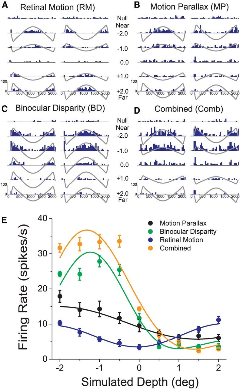
Raw data from an example MT neuron. A, PSTHs (blue bars) for the RM condition. The left and right columns correspond to the two starting phases of simulated observer motion. The top row shows PSTHs for the “null” condition in which no dots were presented in the receptive field. The remaining rows show PSTHs for 5 of the 9 simulated depths that were tested. Gray curves show the retinal velocity profile of each stimulus. B–D, PSTHs are shown, in the same format as A, for the MP condition, the BD condition, and the Comb condition, respectively. E, Depth tuning curves are shown for the same example neuron for the RM (blue), MP (black), BD (green), and Comb (orange) conditions. Each tuning curve plots mean firing rate (averaged across the duration of the trial as well as the two starting phases of motion) against simulated depth of the stimulus. Error bars indicate SEM.

In the Retinal Motion (RM) condition, the visual image (relative to the fixation target) was identical to that of the MP condition but the monkey was not translated by the motion platform and the monkey did not need to move its eyes to maintain fixation. In this control condition, the visual image was generated by translating the OpenGL camera along the same trajectory that the monkey followed in the MP condition. As the OpenGL camera translated, it also rotated to maintain “aim” at the fixation target. This simulates the smooth tracking eye movements of the animal, and generates visual stimuli that match those in the MP condition (assuming accurate smooth pursuit). The monkey performed 6–10 repetitions of each stimulus condition at each simulated depth, randomly interleaved. Because retinal stimulation was essentially the same between the MP and RM conditions (assuming accurate pursuit, see Nadler et al., 2008), any differences in neural responses should be due to extraretinal signals.

In the MP and RM conditions, visual stimuli were viewed monocularly and no binocular depth cues were present. In contrast, the Binocular Disparity (BD) condition was used to determine the disparity tuning of the neuron. This condition involved no platform or camera movement and the visual stimulus (again, a circular patch of random dots) was viewed dichoptically. Stereoscopic images were created by using two OpenGL cameras that were separated horizontally by one interocular distance (Monkey 1 = 3.1 cm, Monkey 2 = 3.5 cm), and stereoscopic presentation was achieved by presenting left and right half-images on alternate video frames. Since many MT neurons respond weakly to stationary random-dot stimuli (Palanca and DeAngelis, 2003) and this condition contained no platform or camera movement, we chose to add some motion to the dots. Using the same movement profile as in the MP condition (a modified sinusoid), the cylinder on which the dots were projected was rotated sinusoidally, while the fixation point and OpenGL camera remained stationary. Thus, the random-dot patch oscillated back and forth along the neuron's preferred-null axis, and the magnitude and direction of the excursion were independent of simulated depth. The movement of the dots (peak retinal velocity = 5 degrees/s) was identical for all depths, and only the amount of binocular disparity varied. As in the MP condition, depths ranged from −2 to +2 degrees in 0.5 degree intervals, for a total of nine simulated depths.

Finally, the Combined (Comb) condition is identical to the MP condition, except that the visual stimuli were presented to both eyes. In this case, both the monkey and a pair of OpenGL cameras were translated. Both binocular disparity and MP cues signaled the same simulated depth. It is important to note, however, that a direct equivalence between motion parallax and disparity cues only holds for horizontal translations of the head. Whereas a single eye can be translated in any direction in the frontoparallel plane to produce motion parallax, binocular disparity is produced by the physical separation of the two eyes, and that separation is always in the horizontal plane of the head. When the axis of translation is horizontal, equivalent disparity is identical to binocular disparity. However, when the axis of motion is not horizontal, the locus of points that has a constant equivalent disparity (an oriented cylinder), does not have a constant binocular disparity. Thus, when the axis of motion is not horizontal in the Comb condition, binocular disparities can vary across the stimulus patch. The range of disparity variation depends mainly on the axis of translation, and to a lesser extent on the retinotopic location of the stimulus patch. Importantly, both disparity and motion parallax cues simulated the same physical surface, and thus were congruent.

Electrophysiological recordings

A bilateral recording grid was placed over the skull, and fixed in place using dental acrylic. Small burr holes were drilled at known stereotaxic locations under general anesthesia. These locations were aligned to the recording grid, such that the electrode was advanced into the brain through a guide tube by a hydraulic microdrive that was mounted above the recording grid. Tungsten microelectrodes (FHC) having a typical impedance of 1–2 MΩ were used to record extracellular activity. Raw neural signals were amplified and bandpass filtered, using an eight-pole filter with cutoff frequencies at 400 Hz and 5 kHz. Action potentials of single units (SUs) were isolated using a window discriminator (Bak Electronics) and their times were recorded with 1 ms resolution.

Multi-unit (MU) activity was extracted off-line, from continuous recordings of the raw neural signals that were sampled at 25 kHz using a CED Power1401 interface. An MU event was defined as any deflection of the analog voltage signal that exceeded a threshold voltage level. The absolute frequency of MU events was arbitrary and changed depending on the level of the event threshold. To achieve some consistency across recording sites, the event level threshold was adjusted such that we obtained an MU spontaneous activity level that was 75 spikes/s greater than the spontaneous activity level of the SU. To make the MU event train independent of the SU spike train, each SU spike was removed (off-line) from the MU event stream. Cross-correlation analyses performed before and after the removal of SU spikes confirmed the success of this manipulation (Chen et al., 2008).

Area MT was recognized based on the following criteria: comparison of gray and white matter transitions along electrode penetrations with structural MRI images of the monkey's brain, response properties of SUs and MU clusters (direction, speed, and disparity tuning), retinal topography, the relationship between receptive field size and eccentricity, and passage through gray matter with response properties typical of the dorsal subdivision of the medial superior temporal (MSTd) before entry into MT.

Data analysis

Data were analyzed using custom software written in MATLAB (MathWorks). For generation of peristimulus time histograms (PSTHs), firing rate was computed in 50 ms bins. To construct depth tuning curves (see Fig. 2), we combined data across the two phases of platform motion and computed mean firing rates within a temporal window matching the total duration of each 2 s trial. This temporal window began 80 ms after stimulus onset and ended 80 ms after stimulus offset (to compensate for response latency).

Figure 2.

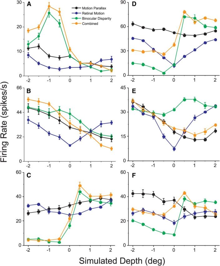
Depth tuning curves for six additional example neurons. Data are shown for six MT cells that show significant selectivity for depth sign based on both motion parallax and binocular disparity cues. Mean firing rates are plotted as a function of simulated depth for the MP (black), RM (blue), BD (green), and Comb (orange) conditions, in the same format as Figure 1E. Error bars indicate SEM. A, B, Neurons that prefer near stimuli in both the MP and BD conditions. C, A neuron that prefers far stimuli in both the MP and BD conditions. D–F, Neurons that exhibit opposite depth-sign preferences for motion parallax and disparity.

Quantification of depth-sign selectivity.

Because the visual motion stimulus in the RM and MP conditions was designed to be depth-sign ambiguous, we focus on quantifying the extent to which MT neurons show selectivity for depth sign (i.e., a preference for near or far). This was quantified by computing a Depth-Sign Discrimination Index (DSDI; Nadler et al., 2008, 2009) as follows:

For each pair of depths symmetric around zero (e.g., ±1 degree), we calculated the difference in response between far (R_far) and near (R_near) depths, relative to response variability (σ_avg, the average SD of the two responses). We then averaged this metric across the four matched pairs of depths to obtain the DSDI, which ranges from −1 to 1. The DSDI metric has the advantage of taking into account trial-to-trial variations in response while quantifying the magnitude of response differences between near and far. Neurons that respond more strongly to near stimuli will have negative DSDI values, whereas neurons that prefer far stimuli will have positive DSDI values. DSDI values were calculated separately for each of the four stimulus conditions. Each DSDI value was classified as significantly different from zero (or not) by permutation test (1000 permutations, p < 0.05; Nadler et al., 2008).

We then categorized cells as “congruent” or “opposite” based on their depth-sign selectivity in the MP and BD conditions. This was done for neurons that showed significant depth tuning (ANOVA, p < 0.05) and DSDI values significantly different from zero (permutation test, p < 0.05) in both the MP and BD conditions. Among cells that met these criteria, congruent cells were defined as those having DSDI values with the same sign for the MP and BD conditions, whereas opposite cells were those for which the DSDI values had opposite signs.

Gabor fits to depth tuning curves.

To quantify and parameterize depth tuning curves, data were fit with a Gabor function (DeAngelis and Uka, 2003) of the form:

where d denotes the depth of the stimulus (in units of degrees of equivalent disparity or binocular disparity), R₀ is the baseline response level, A is the tuning curve amplitude, d₀ is the depth at the center of the Gaussian envelope, σ is the SD of the Gaussian envelope, f is the frequency of the sinusoid, and Φ is the phase of the sinusoid.

The frequency parameter, f, was varied only within a range of ± 10% around the peak of the Fourier transform of the raw depth tuning curve. This improved convergence of the optimization with minimal increase in the overall error of the fits (DeAngelis and Uka, 2003). Overall, the Gabor function provided excellent fits to depth tuning curves of MT neurons, accounting for 87% (median) of the variance in the data for the MP condition, 90% for the BD condition, and 91% for the Combined condition.

Eye movement analyses.

Horizontal and vertical eye position signals (which were sampled at 250 Hz) were differentiated to compute horizontal and vertical eye velocity signals. For quantification of pursuit eye movements, we then computed eye velocity along the axis of the eye movement (which was determined by the direction tuning of each neuron). Pursuit gain was computed to measure how accurately the animal tracks the smooth motion of the fixation target in the MP and Comb conditions. To calculate pursuit gain, we used Fourier analysis to compute the amplitude of the 0.5 Hz component of the average measured eye velocity, and we divided this by the amplitude of the 0.5 Hz component of the target (FP) velocity (0.5 Hz is the fundamental frequency). Pursuit gain values < 1.0 reflect underpursuit and values > 1.0 indicate overpursuit. When binocular eye movement signals were available, pursuit gain was computed from the average velocity of the two eyes.

Eye movement signals were available from both eyes for virtually all recording sessions from Monkey 1 (78/79) and for a small subset (10/55) of recording sessions from Monkey 2. We computed vergence error as the difference in eye position between the left and right eyes. This difference signal was averaged over the course of each stimulus presentation to compute an average vergence error for each trial. If the monkey's eyes are correctly converged on the fixation target (in the plane of the display), then the vergence error is expected to be zero.

Results

To understand the relationships between selectivity for depth based on motion parallax and binocular disparity cues, we measured depth tuning curves for MT neurons in four stimulus conditions: the MP condition in which depth from motion was disambiguated by extraretinal cues (namely eye movements; Nadler et al., 2009); the RM condition in which no extraretinal cues were present and depth sign from motion parallax was ambiguous; the BD condition in which depth was specified only by binocular disparity; and the Comb condition in which binocular disparity cues were added to the motion parallax stimulus of the MP condition. We recorded from any MT neuron for which action potentials could be isolated, even though some cells had poor responses to the range of speeds that were present in the motion parallax stimuli (up to ∼5 deg/s). Our dataset includes extracellular recordings from 133 well isolated SUs that were tested under all four stimulus conditions described above and one additional cell that was tested under three of the four conditions (MP, RM, and BD).

Example neurons

Figure 1, A–D, shows PSTHs of responses of an example MT neuron to stimuli presented in the four stimulus conditions described above (MP, RM, BD, and Comb). The responses are grouped into columns according to the starting phase of the real or simulated self-motion (see Materials and Methods; Nadler et al., 2008). In the RM condition (Fig. 1A), responses of the example neuron largely follow the retinal velocity profiles of the visual stimuli (gray curves), with robust responses to retinal motion in the preferred direction (positive deflections of the gray curves) and little response during motion in the null direction (negative deflections). Because the visual stimuli in the RM condition are depth-sign ambiguous, near and far simulated depths of equal magnitude (e.g., −2° vs +2°) produce similar levels of neural activity. When mean firing rates (averaged across time and starting phases of motion) are plotted as a function of simulated depth, the depth tuning curve for the RM condition (Fig. 1E, blue) is symmetrical around zero. The curve is U-shaped because the speed of retinal image motion increases with the magnitude of simulated depth, and this neuron preferred speeds larger than that corresponding to the largest depth tested (∼5 deg/s). Thus, as expected from the design of the stimuli, the response of the example MT neuron is depth-sign ambiguous in the RM condition.

In striking contrast, the same neuron shows a very different pattern of responses in the MP condition (Fig. 1B), even though the retinal velocity profiles of the stimuli are the same. In the MP condition, this example neuron shows elevated responses to near-simulated depths and suppressed responses to far simulated depths. This yields a clearly asymmetrical depth tuning curve (Fig. 1E, black) in which responses decrease monotonically from near to far. Thus, as shown previously (Nadler et al., 2008), many MT neurons combine extraretinal signals with retinal image motion to signal depth sign from motion parallax.

The main goal of this study is to compare depth tuning in the MP condition with that obtained by presenting stimuli with different binocular disparities. Figure 1C shows responses of the example neuron to stimuli of various depths in the BD condition. Note that, for the BD stimuli, all simulated depths have identical retinal velocity profiles, and only the disparity varies. The response of this neuron to the BD condition is strong for near depths and declines sharply as disparities become positive (far). Thus, the depth tuning curve in the BD condition (Fig. 1E, green) is fairly similar in shape to that of the MP condition (black), and we refer to such neurons as “congruent” cells.

Finally, Figure 1D shows responses of the example neuron in the Comb condition. This condition is identical to the MP condition except that the stimulus is presented to both eyes and contains binocular disparity cues. The cell's pattern of response is very similar to that seen for the BD condition, but there is substantially greater response modulation for near depths. As a result, the depth tuning curve in the Comb condition (Fig. 1E, orange) has a similar shape but a greater peak-to-trough response differential than the tuning curve in the BD condition. For this neuron, it is therefore clear that motion parallax and binocular disparity cues interact to enhance depth selectivity, but we shall see that other outcomes also occurred frequently.

Tuning curves for six additional example neurons are shown in Figure 2. All of these neurons show significant selectivity for depth sign in the MP and BD conditions (permutation test, p < 0.05). If MT neurons represent depth in a cue-invariant fashion, then we expect depth-sign preferences to be matched in the MP and BD conditions, as was the case in Figure 1. This was often the case, as illustrated by the example neurons shown in Figure 2A–C. However, we also found numerous examples of MT neurons with opposite depth-sign preferences for the two cues (Fig. 2D–F).

In the Comb condition, depth tuning depended substantially on the congruency between tuning in the MP and BD conditions. For neurons with matched depth-sign preferences, depth tuning in the Comb condition was generally similar to that of one or both of the individual cues (Fig. 2A–C, orange curves). For these congruent cells, the peak-to-trough response modulation in the Comb condition was generally larger than that for the MP and BD conditions (Fig. 2A–C). For neurons with opposite depth-sign preferences for the two cues (“opposite cells”), various patterns of Comb tuning were observed. For cells such as that in Figure 2D, tuning in the Comb condition closely resembled that of the BD condition. In other opposite neurons, Comb tuning closely followed that of the MP condition and the disparity cue appeared to have little effect (Fig. 2E). Finally, many neurons showed tuning in the Comb condition that was intermediate, reflecting the contributions of both the motion parallax and binocular disparity cues to varying extents (Fig. 2F).

It is clear from the example neurons in Figure 2 that depth tuning curves measured in the MP and BD conditions often have different shapes, even when they share a common depth-sign preference (Fig. 2A,C). Consistent with previous quantitative reports (Maunsell and Van Essen, 1983; DeAngelis and Uka, 2003), many MT neurons have disparity tuning curves with well defined peaks and troughs over the disparity range tested, whereas depth tuning curves for the MP condition are typically monotonic (Nadler et al., 2008, 2009). To summarize the degree of similarity between the shapes of depth tuning curves for the MP, BD, and Comb conditions, we computed correlation coefficients between the tuning curves (mean firing rate at nine depths) for all three pairs of these conditions. Comparing tuning curves for the MP and BD conditions (Fig. 3A), we find that correlation coefficients are broadly distributed, with a median value (0.017) that is not significantly different from zero (p = 0.495 Wilcoxon rank-sum test) and approximately equal numbers of positive and negative correlations. This likely reflects the approximately equal proportions of congruent and opposite cells in MT, as described below, as well as differences in the shape of depth tuning curves in the MP and BD conditions. Comparing depth tuning in the Comb condition with that in the MP (Fig. 3B) or BD (Fig. 3C) conditions, we find a much greater prominence of positive correlations, with median correlation coefficients of 0.483 for Comb versus MP and 0.715 for Comb versus BD (both of which are significantly greater than zero, p < 0.0001 Wilcoxon rank-sum test). Moreover, the median R value for Comb versus BD is significantly greater than that for Comb versus MP (p < 0.05, Wilcoxon signed-rank test), indicating that Comb tuning tends to be more similar to BD tuning for a greater proportion of neurons (Fig. 2A,C,D). As shown by the representative examples in Figure 2, many neurons have sharper peaks and/or steeper slopes in their BD tuning curves, as compared with MP curves, and the Comb responses often seem to reflect these prominent features of the disparity tuning. Figure 3D shows the Comb versus BD correlation coefficient plotted against the Comb versus MP correlation coefficient, for all neurons. There is no significant correlation between the variables (r = −0.15, p = 0.09), and no clear tendency for congruent or opposite cells to have Comb tuning that is more strongly correlated with BD or MP tuning.

Figure 3.

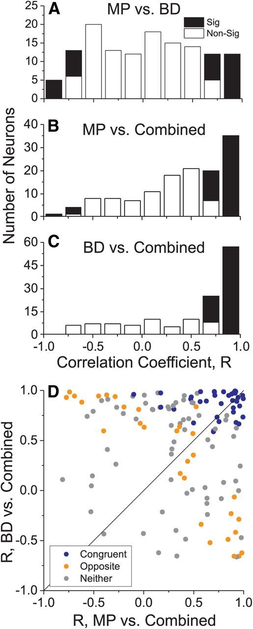
Summary of similarity of tuning curve shapes across stimulus conditions. For each neuron (N = 133), we computed the Pearson correlation coefficient (R) between depth tuning curves for each pairing of the MP, BD, and Comb conditions. Filled bars denote correlations that were significantly different from zero (p < 0.05). A, MP versus BD conditions. The distribution of correlation coefficients was very broad, indicating no systematic tendency for depth tuning to be similar in the MP and BD conditions. B, MP versus Comb conditions. The shift toward positive R values indicates that Comb tuning is similar in shape to MP tuning for many cells. C, BD versus Comb conditions. The larger shift toward positive R values indicates that Comb tuning tends to be more similar to BD tuning than MP tuning. D, Scatter plot showing the correlation coefficient for BD versus Comb against the correlation coefficient for MP versus Comb. Symbol colors denote congruent (blue, N = 37), opposite (orange, N = 29), and unclassified (gray, N = 67) cells.

Given that Comb tuning is often similar to BD tuning for many cells, one may wonder whether the Comb responses of MT neurons could simply be predicted from a combination of BD and RM tuning, without any substantive contribution from the extraretinal signals that generate depth-sign selectivity in the MP condition. To examine this issue, we attempted to fit Comb responses as a weighted sum of either RM and BD responses, or MP and BD responses as follows:

where R_Comb, R_RM, R_MP, and R_BD denote responses in the Comb, RM, MP, and BD conditions, respectively. W_RM, W_MP, and W_BD are free parameters that denote the weights applied to the individual cue responses, and C is a constant free parameter. We found that the median R² value of the fits was 0.64 for Equation 3 and 0.79 for Equation 4, and this difference was highly significant (Wilcoxon matched-pairs test, p < 10⁻⁶). Thus, it is clear that extraretinal signals make a substantial contribution to depth tuning in the Comb condition.

Population summary of depth-sign selectivity

To quantify the depth-sign selectivity of MT neurons, we computed a DSDI (see Materials and Methods; Nadler et al., 2008). This index measures the relative strength of responses to near and far stimuli, and ranges from −1 to +1 with negative values denoting a near preference and positive values indicating a far preference. Figure 4A shows a comparison of DSDI values between the MP and BD conditions for our sample of 134 MT neurons. Among these, 72% (97/134) showed significant depth-sign selectivity in the MP condition while 64% (86/134) expressed significant depth-sign selectivity in the BD condition (permutation test, p < 0.05). Since DSDI only measures a neuron's near/far preference, we also used ANOVA to assess the significance of depth tuning. This revealed that 54% (73/134) of MT neurons showed significant depth tuning in the MP condition, and 72% (96/134) showed significant tuning in the BD condition. The greater incidence of significant BD selectivity by ANOVA versus DSDI is not surprising because some MT neurons have BD tuning curves that peak near zero disparity (DeAngelis and Uka, 2003), whereas peaked tuning in the MP condition is very uncommon (Nadler et al., 2008). In contrast, ANOVA yielded fewer significantly tuned cells than DSDI for the MP condition, presumably because the DSDI measure is more sensitive due to pooling of responses across depths.

Figure 4.

Comparison of depth-sign selectivity and depth preferences between the MP and BD conditions. A, The DSDI for the BD condition (ordinate) is plotted against the DSDI value for the MP condition (abscissa) for each neuron in our sample (N = 134). Filled black symbols indicate DSDI values that are significantly different from zero (p < 0.05, permutation test) in both the MP and BD conditions. Filled red symbols indicate DSDI values that are significantly different from zero in the MP condition, but not in the BD condition. Open black circles indicate DSDI values that are significantly different from zero in the BD condition, but not in the MP condition. Finally, open red circles indicate DSDI values that are not significantly different from zero in either the BD or MP conditions. Cells with near-horizontal direction preferences (within 30 degrees of the horizontal meridian) are represented by triangles (N = 39) while all other cells are represented by circles. B, Scatter plot showing the preferred depth for the BD condition plotted against that for the MP condition. Data are shown for all neurons with significant depth tuning (ANOVA, p < 0.05) in both the MP and BD conditions (N = 52). Symbol colors indicate congruent (blue, N = 31), opposite (orange, N = 13), and unclassified (gray, N = 8) cells. Cells with near-horizontal direction preferences are again represented by triangles while all other cells are represented by circles. Marginal histograms show distributions of depth preferences for congruent, opposite, and unclassified neurons.

Overall, 66/134 MT neurons had significant depth-sign selectivity (DSDI values significantly different from zero) for both the MP and BD conditions (Fig. 4A, filled black symbols). Among these neurons selective for both cues, 56% (37/66) had the same depth-sign preference for the MP and BD conditions (Fig. 4A, data points in the upper right and lower left quadrants). The remaining 44% (29/66) had opposite depth-sign preferences for the two cues (upper left and lower right quadrants), with the majority preferring near depths for motion parallax and far depths for disparity. Across the entire population, there is a weak but significant correlation between DSDIs for the MP and BD conditions (r = 0.24, p = 0.005; Spearman correlation). Thus, MT neurons on the whole show only a modest tendency to have matched depth tuning for motion parallax and disparity cues.

One potential reason for mismatches between MP and BD tuning may be the stimuli themselves. The axis of head translation is tailored to the preferred direction of the neuron from which we are recording, and the stimuli are portions of a cylinder whose long axis is perpendicular to the axis of translation (so that retinal motion is depth-sign ambiguous; Nadler et al., 2008). When the direction of head translation is horizontal (left or right), the stimuli lie on a vertical cylinder whose cross section is a locus of constant horizontal disparity (i.e., the Vieth–Müller circle). Thus, for horizontal head movements, each visual stimulus contains a single binocular disparity value. In contrast, when head motion has a vertical component, the visual stimulus for a given simulated depth contains a range of disparity values. Hence it is possible that neurons with mismatched MP and BD tuning are cells with preferred directions of motion that have a substantial vertical component.

To address this issue, we examined data from a subset of cells (39 neurons) that had preferred directions within ±30 deg of horizontal. DSDI values for those neurons are represented in Figure 4A as triangles. Twenty of these 39 neurons had significant DSDI values for both the MP and BD conditions. Of these, 60% (12/20) had the same sign of depth preference for MP and BD conditions, compared with 56% for the full population. The remaining 40% (8/20) had opposite depth-sign preferences for the two cues, compared with 44% of the full population. The proportion of congruent cells among this subset of horizontal-preferring neurons was not significantly different from that of the full population (p = 0.755; χ² test). Moreover, in this subset, there was no significant correlation between DSDIs for the MP and BD conditions (r = 0.11, p = 0.64; Spearman correlation). To further assess the above hypothesis for the entire sample of neurons, we examined the relationship between direction preference (relative to horizontal) and the absolute difference in DSDI between the MP and BD conditions, and we found no significant correlation (r = −0.06, p = 0.49; Spearman rank correlation). Thus, it is clear that many MT neurons have mismatched depth-sign preferences for the MP and BD conditions and that this cannot simply be attributed to direction preferences.

Next, we examined the relationship between preferred depth values for the MP and BD conditions. For each neuron with significant depth tuning (ANOVA, p < 0.05) in both the MP and BD conditions (N = 52), we fit the tuning curve with a Gabor function (see Materials and Methods) and determined the depth at which the cell produced the greatest response. Consistent with previous studies (DeAngelis and Uka, 2003), the distribution of preferred binocular disparities is broad and centered around zero disparity (Fig. 4B, right marginal histogram). In contrast, the distribution of depth preferences in the MP condition is clearly bimodal, with neurons responding best to either large near or large far depths (Fig. 4B, top marginal histogram). This is consistent with the observation that MP tuning is generally monotonic in MT (Nadler et al., 2008, 2009).

For neurons with significant depth tuning in both MP and BD conditions, the relationship between depth preferences depends strongly on congruency, as expected. For congruent cells (Fig. 4B, blue symbols), data generally fall in the upper right and lower left quadrants, whereas data fall in the upper left and lower right quadrants for opposite cells (orange). Gray symbols denote cells that cannot be classified as either congruent or opposite, and most of these have a preferred depth near zero for the BD condition.

Effect of cue combination on depth-sign selectivity

We now consider whether responses to combinations of motion parallax and binocular disparity cues (Comb condition) show enhanced depth-sign selectivity relative to the single-cue conditions. Since the stimulus in the Comb condition is the MP stimulus with added disparity, we first compare DSDI values between the Comb and MP conditions. As shown in Figure 5A, DSDI values are strongly correlated between Comb and MP conditions across the whole sample of neurons (r = 0.78, p < 0.0001, Spearman rank correlation). Among cells with significant depth-sign selectivity in both conditions, the vast majority have matched depth-sign preferences (Fig. 5A, filled black symbols in upper right and lower left quadrants). To compare the strength of selectivity across conditions, independent of sign, we plotted the absolute values of DSDI in Figure 5C. Across the entire sample of MT neurons, mean values of |DSDI| are 0.40 ± 0.02se for the MP condition and 0.46 ± 0.02se for the Comb condition, and this difference was significant (p = 0.01; Wilcoxon signed-rank test). When considering congruent neurons alone (Fig. 5C, blue symbols), the difference in |DSDI| becomes larger and more significant, with mean values of 0.71 ± 0.03se for the Comb condition and 0.56 ± 0.02se for the MP condition (p < 0.0001; Wilcoxon signed-rank test). In contrast, for opposite cells, the mean value of |DSDI| for the Comb condition (0.44 ± 0.04se) was smaller than that for the MP condition (0.51 ± 0.03se), although the difference did not reach significance (Fig. 5C, orange symbols; p = 0.11). Thus, adding disparity cues to the MP stimulus improves depth-sign selectivity for congruent cells, but not for opposite cells.

Figure 5.

Comparison of depth-sign selectivity between the single-cue conditions and the Comb condition. A, DSDI values for the Comb condition are plotted against those for the MP condition. All neurons are included (N = 133) except for one cell for which the Comb condition was not tested. Filled black symbols denote cells with significant selectivity in both conditions (permutation tests, p < 0.05), whereas filled red symbols denote cells with significantly selectivity for the MP condition only. Open black symbols indicate cells with significant selectivity in the Comb condition, whereas open red symbols indicate that selectivity was significant in neither condition. B, DSDI values for the Comb versus BD conditions. Format as in A. C, The absolute value of DSDI for the Comb condition is plotted against absolute DSDI for the MP condition (N = 133). Symbol colors denote congruent (blue, N = 37), opposite (orange, N = 29), and unclassified (gray, N = 67) cells. D, The absolute value of the DSDI for the Comb condition versus that for the BD condition. Same format as C.

Similar results were obtained for a comparison of depth-sign selectivity between the Comb and BD conditions, although it should be noted at the outset that the stimulus in the Comb condition is not simply the result of adding motion parallax to the BD stimulus (see Materials and Methods). Nevertheless, DSDI values were robustly correlated between the Comb and BD conditions (Fig. 5B, r = 0.61, p < 0.0001; Spearman rank correlation). Considering the absolute value of DSDI for all neurons, there was only a marginally significant difference in |DSDI| between the Comb condition (0.46 ± 0.02se) and the BD condition (0.42 ± 0.02se, p = 0.053; Wilcoxon signed-rank test). For congruent cells, however, |DSDI| was significantly greater in the Comb condition (0.71 ± 0.03se) than in the BD condition (0.63 ± 0.03se, Fig. 5D, blue symbols; p = 0.007; Wilcoxon signed-rank test). For opposite cells, there was a marginally significant trend in the other direction, such that the average |DSDI| in the Comb condition (0.44 ± 0.04se) was less than that measured in the BD condition (0.55 ± 0.03se, Fig. 5D, orange symbols; p = 0.04). Overall, these findings suggest that combining motion parallax and binocular disparity cues improves depth-sign selectivity, but only for congruent cells.

Clustering of depth tuning properties

It is well established that adjacent neurons in visual cortex often share similar tuning properties and may be organized in columnar structures (Hubel and Wiesel, 1962, 1963; Freeman, 2003; Horton and Adams, 2005). In area MT, previous work has shown that there is clustering of neurons according to tuning for direction (Albright et al., 1984; Malonek et al., 1994), speed (Liu and Newsome, 2003), and disparity (DeAngelis and Newsome, 1999). Here, we examine whether there is clustering of depth tuning based on motion parallax, and compare it to clustering for binocular disparity.

To assess clustering, we compared the depth tuning of SU and MU activity recorded simultaneously from a single electrode in area MT. MU events were defined by thresholding the raw neural signals (see Materials and Methods), and SU spikes were removed from the MU event train such that MU responses reflect the activity of neurons that are nearby the SU. Independence of MU and SU activity (following subtraction of SU events from the MU record) was confirmed by computing cross-correlograms, as described previously (Chen et al., 2008). If MU activity generally has depth tuning properties similar to SU activity, this would provide evidence that depth tuning properties are clustered in MT.

Examples of SU and MU depth tuning curves are shown for two different recording sites in Figure 6. For both the BD (blue) and MP (red) conditions, depth tuning curves are closely matched for MU and SU activity. Note that the peak MU response is ∼3-fold larger than the peak SU response for the recording of Figure 6A, and ∼10-fold larger for the recording of Figure 6B. These examples suggest that depth tuning properties are clustered in MT.

Figure 6.

Comparison of SU and MU depth tuning curves. Data are shown for two example recording sites in MT (A and B). Depth tuning curves are shown for the MP (red) and BD (blue) conditions. Filled symbols represent SU responses whereas open symbols denote MU responses. Error bars indicate SEM.

Figure 7 summarizes the relationships between depth tuning parameters derived from MU and SU activity. A comparison of peak responses (at the preferred depth) between MU and SU responses is shown in Figure 7A for the MP condition and in Figure 7B for the BD condition. For the MP condition, the average peak response of MU activity (135.5 ± 5.3 SEM impulses/s) was almost fivefold greater than the average peak response for SUs (25.7 ± 1.6 spikes/s). Results were similar for the BD condition (mean MU response: 145.4 ± 6.3 impulses/s; mean SU response: 27.5 ± 1.5 spikes/s). In addition, the average difference in response between the peak and trough of the depth tuning curve was much greater for MU activity (MP: 39.1 ± 2.2 impulses/s; BD: 66.6 ± 5.1 impulses/s) than for SU activity (MP: 8.4 ± 0.5 spikes/s; BD: 14.2 ± 1.1 spikes/s). Together, these data suggest that action potentials from multiple SUs contributed to most of our MU recordings.

Figure 7.

Comparison of MT response properties between SU and MU activity. A, The peak response of MU activity is plotted against the peak SU response, for the MP condition. Data points lie well above the unity-slope diagonal indicating substantially larger MU than SU responses. Data are shown for all recording sites for which MU activity was available (N = 119). B, Comparison of SU and MU peak responses for the BD condition (N = 117). Format as in A. C, DSDI values are compared between MU and SU responses for the MP condition. Same dataset as in A (N = 119). D, Comparison of MU and SU DSDI values for the BD condition (N = 117). E, The preferred depth for MU activity is plotted against the corresponding preferred depth for SU activity. Preferred depths were obtained as the peak of the best-fitting Gabor function (see text). Data are shown for the subset of recording sites for which depth tuning was significant for both MU and SU activity (ANOVA, p < 0.05, N = 47). F, Comparison of MU and SU depth preferences for the BD condition (N = 74).

Figure 7, C and D, compares DSDI values derived from SU and MU responses for the MP and BD conditions, respectively. MU and SU DSDI values were strongly correlated in both the MP (r = 0.78, p < 0.0001, Spearman rank correlation) and BD (r = 0.82, p < 0.0001) conditions. There was a marginally significant difference between MU and SU DSDI values for the MP condition (Wilcoxon signed-rank test, p = 0.02), with no significant difference for the BD condition (p = 0.2). For the absolute value of DSDI, there was no significant difference between SU and MU activity for either stimulus condition (Wilcoxon signed-rank test, MP: p = 0.45, BD: p = 0.43, data not shown). These results show that depth sign selectivity is generally quite similar for SU and MU activity in MT.

Next, we compared SU and MU depth preferences. For this analysis, we selected only recording sites that showed significant depth tuning (ANOVA, p < 0.05) for both MU and SU responses (N = 47 for the MP condition and N = 74 for the BD condition). For each such recording site, we fit tuning curves with Gabor functions (Fig. 1E) and defined the preferred depth as that corresponding to the peak of the fitted curve. Figure 7E compares depth preferences for SU and MU responses in the MP condition. Because most MP tuning curves are monotonic, preferred depths tend to cluster around large positive or negative values. SU and MU depth preferences are strongly correlated for the MP condition (r = 0.80, p < 0.0001, Spearman rank correlation), indicating that MT neurons are strongly clustered according to whether they prefer near or far stimuli based on motion parallax. For the BD condition, depth preferences are more broadly distributed (Fig. 7F) and are generally well matched between MU and SU responses (r = 0.82, p < 0.0001), as expected from previous work (DeAngelis and Newsome, 1999). Together, the data of Figure 7 demonstrate that MT neurons are robustly clustered according to their depth tuning for motion parallax, and the strength of this clustering is similar to that seen for binocular disparity tuning.

If depth preferences are clustered in both the MP and BD conditions, and this is true for both congruent and opposite cells, this suggests that MT neurons should also be clustered according to the congruency of their depth tuning for disparity and motion parallax. Indeed, this was found to be the case. The vertical axis of Figure 8 shows the difference between DSDI values computed from MU responses in the MP and BD conditions, and the horizontal axis shows the corresponding difference between DSDI values computed from SU activity at the same recording sites. Data are color coded according to the congruency of SU depth tuning at each site. A robust correlation is observed in this plot (r = 0.80, p < 0.001, N = 117), indicating that the congruency of depth tuning is strongly clustered in MT. Data from congruent cells lie near the origin in this plot, indicating that they have similar DSDI values in the MP and BD conditions for both MU and SU activity. In contrast, opposite cells lie near the extremes of the cluster of data points in Figure 8. Importantly, almost all opposite cells lie in the top right or bottom left quadrants, indicating that their mismatched depth preferences have the same sign relationships for both MU and SU responses.

Figure 8.

MT neurons are clustered according to the congruency of their depth tuning for disparity and motion parallax. For each recording site for which MU activity was available for MP and BD conditions (N = 117), we computed the difference between the DSDI value for the MP condition (DSDI_MP) and that for the BD condition (DSDI_BD). This difference was computed from both MU activity (vertical axis) and SU activity (horizontal axis). Data points are color coded according to the congruency of SU responses, as in Figure 4B. For congruent cells (blue), the difference in DSDI is close to zero for both SU and MU activity because depth-sign preferences are well matched. For opposite cells (orange), negative values of the DSDI difference indicate a far preference for the BD condition and a near preference for the MP condition, whereas positive differences indicate a near BD preference and a far MP preference. The robust correlation in this scatter plot (see text for details) indicates clustering according to MP–BD congruency.

Eye movement analyses

We previously performed extensive analyses of eye movements in the MP and RM conditions (Nadler et al., 2008) and showed that depth-sign selectivity could not be accounted for by inaccurate pursuit. However, it is important to examine whether differences in pursuit gain between stimulus conditions (e.g., MP vs Combined) might account for differences in depth-sign selectivity. In addition, it is important to rule out that variations in the vergence posture of the eyes could account for differences in depth tuning between MP, BD, and Comb conditions.

To quantify the quality of pursuit, we computed pursuit gain from eye velocity traces (see Materials and Methods). The average pursuit gain (across 134 sessions) was 0.953 ± 0.003 SEM for the MP condition and 0.966 ± 0.003 SEM for the Comb condition (133 sessions), and this difference was significant (p < 0.01, Wilcoxon signed rank test). Thus, pursuit gain was significantly greater (closer to the idealized gain of 1.0) in the Comb condition. Importantly, this difference is in the wrong direction to account for the greater DSDI values exhibited by MT neurons in the Comb condition relative to the MP condition. As shown previously (Nadler et al., 2008), underpursuit (pursuit gain < 1) could enhance the depth-sign selectivity of neurons; thus, the slightly greater pursuit gain observed in the Comb condition suggests that the difference in DSDI values between the Comb and MP conditions (Fig. 5C) may indeed be underestimated. Critically, we found no significant correlation between DSDI and pursuit gain for either the MP (r = 0.11, p = 0.22, N = 134) or Comb (r = 0.06, p = 0.47, N = 133) conditions, consistent with previous results for the MP condition (Nadler et al., 2008).

Many MT neurons showed strikingly different depth tuning in the MP and BD conditions. Given that visual stimuli were viewed monocularly in the MP condition and binocularly in the BD and Comb conditions, it is important to exclude the possibility that uncontrolled variations in vergence posture might account for the differences in depth tuning across conditions. For this purpose, we analyzed binocular eye movements obtained during 78 sessions from Monkey 1 and 10 sessions from Monkey 2 (see Materials and Methods). First, we found that there was no significant correlation between vergence error and stimulus depth for any of the stimulus conditions (RM: r = 0.01, p = 0.80; MP: r = 0.01, p = 0.87; BD: r = 0.00, p = 0.92; Comb: r = 0.00, p = 0.97; data pooled across 88 sessions for each condition), indicating that vergence posture was not systematically influenced by stimulus depth. Second, the average vergence error (in degrees, positive indicates convergence nearer than the fixation point) was small across all stimulus conditions for both animals (RM: 0.073 ± 0.042 SEM for Monkey 1, and −0.138 ± 0.045 for Monkey 2; MP: 0.176 ± 0.041 for Monkey 1, and −0.072 ± 0.047 for Monkey 2; BD: 0.041 ± 0.041 for Monkey 1, and −0.131 ± 0.054 for Monkey 2; Comb: 0.078 ± 0.041 for Monkey 1, and −0.118 ± 0.054 for Monkey 2). These small differences in vergence posture between stimulus conditions could not possibly account for the large differences in depth preference between the MP and BD conditions that were exhibited by many neurons (Fig. 4B). Moreover, the difference in vergence error between the MP and BD conditions was not significantly greater for opposite cells than congruent cells (Wilcoxon rank-sum test, p = 0.53). Third, there was no significant correlation between vergence error and the DSDI values of MT neurons for any of the stimulus conditions (RM: r = −0.06, p = 0.57; MP: r = −0.14, p = 0.21; BD: r = −0.02, p = 0.88; Combined: r = −0.12, p = 0.28; data from 88 sessions for each stimulus condition). This indicates that the small variations in vergence error from session to session were not predictive of depth-sign selectivity.

In our experimental design, the fixation window around the target shrunk after 250 ms to allow the animal to initiate pursuit and catch up to the target. Since initial pursuit lags the target, there will be some offset of the visual stimulus relative to the receptive field in the initial 250 ms of each trial. To assess the magnitude of this transient stimulus offset, we computed the position error between eye and target during the initial 250 ms of pursuit, and this error averaged 0.69 deg ± 0.03 SEM. In comparison, receptive field diameters ranged from 7 to 30 deg, with a median value of 11 deg. Thus, as a fraction of receptive field diameter, the position offset of the stimulus during pursuit initiation ranged from 0.02 to 0.15, with a median value of 0.05 (or 5%). Thus, during pursuit initiation, the offset of the stimulus relative to the receptive field was quite small and therefore had little effect on response magnitudes.

Together, these analyses suggest strongly that none of our main conclusions are confounded by imperfections in pursuit gain or variations in either pursuit gain or vergence error between stimulus conditions.

Discussion

It is well established that most MT neurons are selective for depth from binocular disparity (Maunsell and Van Essen, 1983; Bradley et al., 1995; DeAngelis and Uka, 2003; Palanca and DeAngelis, 2003; Ponce et al., 2008; Krug and Parker, 2011), and we previously reported that many MT neurons are also selective for depth defined by motion parallax (Nadler et al., 2008, 2009). Here, we examined whether single MT neurons are selective for each cue individually and how their depth selectivity improves when disparity and motion parallax cues are combined. We found that many neurons show depth selectivity for both motion parallax and disparity, but their depth-sign preferences can be either congruent or opposite. For congruent cells, depth-sign selectivity is enhanced when MP and BD cues are combined, but this does not occur for opposite cells. Finally, we observed that neurons are clustered in MT according to their depth preferences for motion parallax, similar to what was found previously for binocular disparity (DeAngelis and Newsome, 1999). These results demonstrate that area MT is involved in constructing a 3D representation of the visual scene based on multiple depth cues, and our findings suggest that MT may play at least a partial role in combining disparity and motion parallax cues to achieve more robust depth perception when observers are in motion.

Potential roles of MT in cue integration for depth perception

In everyday life, the visual system infers the 3D structure of the environment from a variety of depth cues, including binocular disparity and motion parallax cues as well as various pictorial depth cues (Howard and Rogers, 1995, 2002). Thus, it is of considerable interest to understand how neurons integrate depth cues. Many psychophysical studies have shown that humans can combine multiple sensory cues near-optimally to maximize behavioral performance (Ernst and Banks, 2002; Alais and Burr, 2004), including multiple cues to 3D visual structure (Jacobs, 1999; Knill and Saunders, 2003; Hillis et al., 2004; Knill, 2007; Girshick and Banks, 2009). Recent studies have demonstrated that monkeys integrate visual and vestibular cues to self-motion in near-optimal fashion (Fetsch et al., 2009), and have uncovered the operations by which single neurons in area MSTd combine visual and vestibular inputs to achieve near-optimal cue integration (Gu et al., 2008; Fetsch et al., 2012). However, little is currently known about how neurons integrate multiple depth cues, such as disparity and motion parallax, to produce robust depth perception.

Although the present study was not designed to examine cue integration directly, it provides the first evidence regarding how binocular disparity and motion parallax cues are combined by single neurons in visual cortex. Our findings demonstrate that MT neurons with congruent depth-sign preferences for motion parallax and disparity show greater depth selectivity when both cues are presented together, whereas this does not occur for opposite cells (Fig. 5). Some potential limitations of this study should be noted, however. Most importantly, the Combined stimulus in our experiment is not a simple sum of stimuli from the BD and MP conditions for a couple of reasons. First, since the primary objective of this study was to compare depth tuning from disparity and motion parallax, we added independent motion to the stimulus in the BD condition to better stimulate neurons and measure their disparity tuning. Second, because we are examining a combination of monocular and binocular cues, adding binocular disparity to our MP condition also entails adding motion information to the second eye. As a result, we cannot directly compare the response of MT neurons in the Comb condition with some function (e.g., a weighted sum) of their responses in the MP and BD conditions. As a result of these considerations, we have mainly focused on comparing depth-sign selectivity in the MP condition with that in the Comb condition, when binocular cues are added. Clearly, future studies should focus on designing experiments that will allow a direct comparison between neural and behavioral measurements of cue integration for motion parallax and binocular disparity cues.

The functional roles of congruent and opposite cells

Perhaps the most salient finding of this study is that the depth tuning of almost half of MT neurons for motion parallax is not consistent with their depth tuning for binocular disparity (Figs. 2, 4). What is the potential functional role of these “opposite” cells, and why might MT contain them along with congruent cells? Since congruent cells show greater depth-sign selectivity when disparity cues are added to motion parallax (Fig. 5C), it is reasonable to speculate that congruent cells may play a role in combining disparity and motion parallax cues to achieve more precise depth perception. However, opposite cells do not attain greater depth-sign selectivity during cue combination (Fig. 5C,D), and thus may not be useful for cue integration.

Our findings in area MT are strongly reminiscent of recent findings regarding visual and vestibular tuning for self-motion (heading) in the dorsal subdivision of area MST. Approximately half of MSTd neurons have congruent heading tuning based on visual and vestibular cues, whereas the remaining half prefer opposite directions of motion defined by optic flow and inertial motion of the body (Gu et al., 2006; Morgan et al., 2008). Notably, a mixture of congruent and opposite self-motion neurons can also be found in other cortical areas, including the ventral intraparietal area (Chen et al., 2011a) and the visual posterior sylvian area (Chen et al., 2011b), suggesting that mixtures of neurons with matched or mismatched tuning may be a common finding in areas of the cerebral cortex that contain spatial representations based on multiple cues.

In monkeys trained to perceptually combine visual and vestibular cues during a heading discrimination task, recent studies have shown that congruent MSTd neurons are able to account for perceptual improvements in discrimination performance during cue combination (Gu et al., 2008), as well as perceptual weighting of visual and vestibular cues according to their relative reliabilities (Fetsch et al., 2012). Opposite cells can account for neither the improvement in sensitivity nor the cue weighting effects (Gu et al., 2008; Fetsch et al., 2012). Correspondingly, responses of congruent cells in MSTd are found to correlate with perceptual decisions regarding heading during cue combination, whereas responses of opposite cells do not (Gu et al., 2008). In comparison to these findings, it seems likely that MT neurons with congruent depth tuning for disparity and motion parallax may be well suited to play a role in perceptual depth-cue integration, whereas cells with opposite depth-sign preferences may not.

What, then, might be the functional role of opposite cells in area MT? When an observer translates, all stationary objects in the scene will have retinal image motion that is determined by the distance of the object and the velocity of self-motion. When the observer maintains visual fixation on a world-fixed target during lateral self-translation, stationary objects nearer than the fixation point will move opposite to the head whereas far objects will move in the same direction as the head. Against this backdrop, consider what happens when an object moves in the world during observer translation (Fig. 9). The retinal image motion of such an object will not correspond to what the brain may expect from the object's distance and the velocity of self-motion. In other words, the local retinal motion of the moving object will not be consistent with that predicted from its binocular disparity and the observer's head velocity. If the brain can detect such a local mismatch between disparity and retinal image motion, it should provide an important signal that an object is moving in the world.

Figure 9.

Schematic illustration of the local discrepancy between disparity and motion cues that can arise for a moving object in the world. In this illustration, an observer maintains visual fixation on the traffic light while moving their head to the right. In this case, all stationary objects in the scene have an image velocity that is determined by their 3D location in the scene (as specified by binocular disparity, for example) and the movement of the observer's head. Stationary near objects move leftward in the image, whereas stationary far objects move rightward in the image. However, a moving object (the car) creates local retinal image motion that is not consistent with that expected from the binocular disparity of the object and the movement of the observer. This local discrepancy between disparity and retinal image motion might be sensed by the relative activity of congruent and opposite cells in MT.

We suggest that MT neurons with opposite depth-sign preferences for disparity and motion parallax may be well suited to detecting such local mismatches between image motion and disparity. An opposite cell should not respond maximally to combinations of disparity and motion parallax associated with objects that are stationary in the world, but may respond maximally when an object moves in the world such that its local retinal motion is opposite to that expected from its location in depth (Fig. 9, the moving car). Therefore, we speculate that the brain may detect moving objects by comparing the activity of congruent cells and opposite cells. Such a mechanism would be particularly useful when object motion is not easily detectable via other cues, such as the relative temporal profiles of object motion and self-motion. Testing this hypothesis is a focus of ongoing studies in our laboratory. More generally, the existence of a mixture of neurons with congruent and opposite selectivities may reflect a general coding strategy that the brain adopts to deal with situations in which visual motion signals need to be parsed according to their underlying causes.

References

- Alais D, Burr D. The ventriloquist effect results from near-optimal bimodal integration. Curr Biol. 2004;14:257–262. doi: 10.1016/S0960-9822(04)00043-0. [DOI] [PubMed] [Google Scholar]
- Albright TD, Desimone R, Gross CG. Columnar organization of directionally selective cells in visual area MT of the macaque. J Neurophysiol. 1984;51:16–31. doi: 10.1152/jn.1984.51.1.16. [DOI] [PubMed] [Google Scholar]
- Ban H, Preston TJ, Meeson A, Welchman AE. The integration of motion and disparity cues to depth in dorsal visual cortex. Nat Neurosci. 2012;15:636–643. doi: 10.1038/nn.3046. [DOI] [PMC free article] [PubMed] [Google Scholar]
- Bradley DC, Qian N, Andersen RA. Integration of motion and stereopsis in middle temporal cortical area of macaques. Nature. 1995;373:609–611. doi: 10.1038/373609a0. [DOI] [PubMed] [Google Scholar]
- Chen A, Gu Y, Takahashi K, Angelaki DE, DeAngelis GC. Clustering of self-motion selectivity and visual response properties in macaque area MSTd. J Neurophysiol. 2008;100:2669–2683. doi: 10.1152/jn.90705.2008. [DOI] [PMC free article] [PubMed] [Google Scholar]
- Chen A, DeAngelis GC, Angelaki DE. Representation of vestibular and visual cues to self-motion in ventral intraparietal cortex. J Neurosci. 2011a;31:12036–12052. doi: 10.1523/JNEUROSCI.0395-11.2011. [DOI] [PMC free article] [PubMed] [Google Scholar]
- Chen A, DeAngelis GC, Angelaki DE. Convergence of vestibular and visual self-motion signals in an area of the posterior sylvian fissure. J Neurosci. 2011b;31:11617–11627. doi: 10.1523/JNEUROSCI.1266-11.2011. [DOI] [PMC free article] [PubMed] [Google Scholar]
- Chowdhury SA, DeAngelis GC. Fine discrimination training alters the causal contribution of macaque area MT to depth perception. Neuron. 2008;60:367–377. doi: 10.1016/j.neuron.2008.08.023. [DOI] [PMC free article] [PubMed] [Google Scholar]
- Cumming BG, DeAngelis GC. The physiology of stereopsis. Annu Rev Neurosci. 2001;24:203–238. doi: 10.1146/annurev.neuro.24.1.203. [DOI] [PubMed] [Google Scholar]
- DeAngelis GC, Newsome WT. Organization of disparity-selective neurons in macaque area MT. J Neurosci. 1999;19:1398–1415. doi: 10.1523/JNEUROSCI.19-04-01398.1999. [DOI] [PMC free article] [PubMed] [Google Scholar]
- DeAngelis GC, Uka T. Coding of horizontal disparity and velocity by MT neurons in the alert macaque. J Neurophysiol. 2003;89:1094–1111. doi: 10.1152/jn.00717.2002. [DOI] [PubMed] [Google Scholar]
- DeAngelis GC, Cumming BG, Newsome WT. Cortical area MT and the perception of stereoscopic depth. Nature. 1998;394:677–680. doi: 10.1038/29299. [DOI] [PubMed] [Google Scholar]
- Ernst MO, Banks MS. Humans integrate visual and haptic information in a statistically optimal fashion. Nature. 2002;415:429–433. doi: 10.1038/415429a. [DOI] [PubMed] [Google Scholar]
- Fetsch CR, Turner AH, DeAngelis GC, Angelaki DE. Dynamic reweighting of visual and vestibular cues during self-motion perception. J Neurosci. 2009;29:15601–15612. doi: 10.1523/JNEUROSCI.2574-09.2009. [DOI] [PMC free article] [PubMed] [Google Scholar]
- Fetsch CR, Pouget A, DeAngelis GC, Angelaki DE. Neural correlates of reliability-based cue weighting during multisensory integration. Nat Neurosci. 2012;15:146–154. doi: 10.1038/nn.2983. [DOI] [PMC free article] [PubMed] [Google Scholar]
- Freeman RD. Cortical columns: a multi-parameter examination. Cereb Cortex. 2003;13:70–72. doi: 10.1093/cercor/13.1.70. [DOI] [PubMed] [Google Scholar]
- Girshick AR, Banks MS. Probabilistic combination of slant information: weighted averaging and robustness as optimal percepts. J Vis. 2009;9(9):8.1–20. doi: 10.1167/9.9.8. [DOI] [PMC free article] [PubMed] [Google Scholar]
- Gu Y, Watkins PV, Angelaki DE, DeAngelis GC. Visual and nonvisual contributions to three-dimensional heading selectivity in the medial superior temporal area. J Neurosci. 2006;26:73–85. doi: 10.1523/JNEUROSCI.2356-05.2006. [DOI] [PMC free article] [PubMed] [Google Scholar]
- Gu Y, DeAngelis GC, Angelaki DE. A functional link between area MSTd and heading perception based on vestibular signals. Nat Neurosci. 2007;10:1038–1047. doi: 10.1038/nn1935. [DOI] [PMC free article] [PubMed] [Google Scholar]
- Gu Y, Angelaki DE, DeAngelis GC. Neural correlates of multisensory cue integration in macaque MSTd. Nat Neurosci. 2008;11:1201–1210. doi: 10.1038/nn.2191. [DOI] [PMC free article] [PubMed] [Google Scholar]
- Hillis JM, Watt SJ, Landy MS, Banks MS. Slant from texture and disparity cues: optimal cue combination. J Vis. 2004;4(12):967–992. doi: 10.1167/4.12.1. [DOI] [PubMed] [Google Scholar]
- Horton JC, Adams DL. The cortical column: a structure without a function. Philos Trans R Soc Lond B Biol Sci. 2005;360:837–862. doi: 10.1098/rstb.2005.1623. [DOI] [PMC free article] [PubMed] [Google Scholar]
- Howard IP, Rogers BJ. Binocular vision and stereopsis. New York: Oxford UP; 1995. [Google Scholar]
- Howard IP, Rogers BJ. Depth perception. Vol. 2. Toronto: I. Porteous; 2002. Seeing in depth. [Google Scholar]
- Hubel DH, Wiesel TN. Receptive fields, binocular interaction and functional architecture in the cat's visual cortex. J Physiol. 1962;160:106–154. doi: 10.1113/jphysiol.1962.sp006837. [DOI] [PMC free article] [PubMed] [Google Scholar]
- Hubel DH, Wiesel TN. Shape and arrangement of columns in cat's striate cortex. J Physiol. 1963;165:559–568. doi: 10.1113/jphysiol.1963.sp007079. [DOI] [PMC free article] [PubMed] [Google Scholar]
- Jacobs RA. Optimal integration of texture and motion cues to depth. Vision Res. 1999;39:3621–3629. doi: 10.1016/S0042-6989(99)00088-7. [DOI] [PubMed] [Google Scholar]
- Julesz B. Foundations of cyclopean perception. Chicago: University of Chicago; 1971. [Google Scholar]
- Knill DC. Robust cue integration: a Bayesian model and evidence from cue-conflict studies with stereoscopic and figure cues to slant. J Vis. 2007;7(7):5, 1–24. doi: 10.1167/7.7.5. [DOI] [PubMed] [Google Scholar]
- Knill DC, Saunders JA. Do humans optimally integrate stereo and texture information for judgments of surface slant? Vision Res. 2003;43:2539–2558. doi: 10.1016/S0042-6989(03)00458-9. [DOI] [PubMed] [Google Scholar]
- Krug K, Parker AJ. Neurons in dorsal visual area V5/MT signal relative disparity. J Neurosci. 2011;31:17892–17904. doi: 10.1523/JNEUROSCI.2658-11.2011. [DOI] [PMC free article] [PubMed] [Google Scholar]
- Liu J, Newsome WT. Functional organization of speed tuned neurons in visual area MT. J Neurophysiol. 2003;89:246–256. doi: 10.1152/jn.00097.2002. [DOI] [PubMed] [Google Scholar]
- Malonek D, Tootell RB, Grinvald A. Optical imaging reveals the functional architecture of neurons processing shape and motion in owl monkey area MT. Proc Biol Sci. 1994;258:109–119. doi: 10.1098/rspb.1994.0150. [DOI] [PubMed] [Google Scholar]
- Maunsell JH, Van Essen DC. Functional properties of neurons in middle temporal visual area of the macaque monkey. II. Binocular interactions and sensitivity to binocular disparity. J Neurophysiol. 1983;49:1148–1167. doi: 10.1152/jn.1983.49.5.1148. [DOI] [PubMed] [Google Scholar]
- Morgan ML, DeAngelis GC, Angelaki DE. Multisensory integration in macaque visual cortex depends on cue reliability. Neuron. 2008;59:662–673. doi: 10.1016/j.neuron.2008.06.024. [DOI] [PMC free article] [PubMed] [Google Scholar]
- Nadler JW, Angelaki DE, DeAngelis GC. A neural representation of depth from motion parallax in macaque visual cortex. Nature. 2008;452:642–645. doi: 10.1038/nature06814. [DOI] [PMC free article] [PubMed] [Google Scholar]
- Nadler JW, Nawrot M, Angelaki DE, DeAngelis GC. MT neurons combine visual motion with a smooth eye movement signal to code depth-sign from motion parallax. Neuron. 2009;63:523–532. doi: 10.1016/j.neuron.2009.07.029. [DOI] [PMC free article] [PubMed] [Google Scholar]
- Naji JJ, Freeman TC. Perceiving depth order during pursuit eye movement. Vision Res. 2004;44:3025–3034. doi: 10.1016/j.visres.2004.07.007. [DOI] [PubMed] [Google Scholar]
- Nawrot M. Eye movements provide the extra-retinal signal required for the perception of depth from motion parallax. Vision Res. 2003a;43:1553–1562. doi: 10.1016/S0042-6989(03)00144-5. [DOI] [PubMed] [Google Scholar]
- Nawrot M. Depth from motion parallax scales with eye movement gain. J Vis. 2003b;3(11):841–851. doi: 10.1167/3.11.17. [DOI] [PubMed] [Google Scholar]
- Nawrot M, Joyce L. The pursuit theory of motion parallax. Vision Res. 2006;46:4709–4725. doi: 10.1016/j.visres.2006.07.006. [DOI] [PubMed] [Google Scholar]
- Nawrot M, Stroyan K. The motion/pursuit law for visual depth perception from motion parallax. Vision Res. 2009;49:1969–1978. doi: 10.1016/j.visres.2009.05.008. [DOI] [PMC free article] [PubMed] [Google Scholar]
- Nover H, Anderson CH, DeAngelis GC. A logarithmic, scale-invariant representation of speed in macaque middle temporal area accounts for speed discrimination performance. J Neurosci. 2005;25:10049–10060. doi: 10.1523/JNEUROSCI.1661-05.2005. [DOI] [PMC free article] [PubMed] [Google Scholar]
- Palanca BJ, DeAngelis GC. Macaque middle temporal neurons signal depth in the absence of motion. J Neurosci. 2003;23:7647–7658. doi: 10.1523/JNEUROSCI.23-20-07647.2003. [DOI] [PMC free article] [PubMed] [Google Scholar]
- Parker AJ. Binocular depth perception and the cerebral cortex. Nat Rev Neurosci. 2007;8:379–391. doi: 10.1038/nrn2131. [DOI] [PubMed] [Google Scholar]
- Ponce CR, Lomber SG, Born RT. Integrating motion and depth via parallel pathways. Nat Neurosci. 2008;11:216–223. doi: 10.1038/nn2039. [DOI] [PMC free article] [PubMed] [Google Scholar]
- Roe AW, Parker AJ, Born RT, DeAngelis GC. Disparity channels in early vision. J Neurosci. 2007;27:11820–11831. doi: 10.1523/JNEUROSCI.4164-07.2007. [DOI] [PMC free article] [PubMed] [Google Scholar]
- Rogers B, Graham M. Motion parallax as an independent cue for depth perception. Perception. 1979;8:125–134. doi: 10.1068/p080125. [DOI] [PubMed] [Google Scholar]
- Rogers B, Graham M. Similarities between motion parallax and stereopsis in human depth perception. Vision Res. 1982;22:261–270. doi: 10.1016/0042-6989(82)90126-2. [DOI] [PubMed] [Google Scholar]
- Rogers BJ, Graham ME. Aftereffects from motion parallax and stereoscopic depth: similarities and interactions. In: Spillman L, Wooten BR, editors. Sensory experience, adaptation, and perception: Festschrift Ivo Kohler. Hillsdale, NJ: Lawrence Erlbaum; 1984. pp. 603–619. [Google Scholar]
- Rogers S, Rogers BJ. Visual and nonvisual information disambiguate surfaces specified by motion parallax. Percept Psychophys. 1992;52:446–452. doi: 10.3758/BF03206704. [DOI] [PubMed] [Google Scholar]
- Tcheang L, Gilson SJ, Glennerster A. Systematic distortions of perceptual stability investigated using immersive virtual reality. Vision Res. 2005;45:2177–2189. doi: 10.1016/j.visres.2005.02.006. [DOI] [PMC free article] [PubMed] [Google Scholar]
- Uka T, DeAngelis GC. Linking neural representation to function in stereoscopic depth perception: roles of the middle temporal area in coarse versus fine disparity discrimination. J Neurosci. 2006;26:6791–6802. doi: 10.1523/JNEUROSCI.5435-05.2006. [DOI] [PMC free article] [PubMed] [Google Scholar]
- Wallach H, Stanton L, Becker D. The compensation for movement-produced changes of object orientation. Percept Psychophys. 1974;15:339–343. doi: 10.3758/BF03213955. [DOI] [Google Scholar]