Scoring by nonlocal image patch estimator for early detection of Alzheimer's disease

Abstract

Detection of Alzheimer's disease (AD) at the first stages of the pathology is an important task to accelerate the development of new therapies and improve treatment. Compared to AD detection, the prediction of AD using structural MRI at the mild cognitive impairment (MCI) or pre-MCI stage is more complex because the associated anatomical changes are more subtle. In this study, we analyzed the capability of a recently proposed method, SNIPE (Scoring by Nonlocal Image Patch Estimator), to predict AD by analyzing entorhinal cortex (EC) and hippocampus (HC) scoring over the entire ADNI database (834 scans). Detection (AD vs. CN) and prediction (progressive — pMCI vs. stable — sMCI) efficiency of SNIPE were studied using volumetric and grading biomarkers. First, our results indicate that grading-based biomarkers are more relevant for prediction than volume-based biomarkers. Second, we show that HC-based biomarkers are more important than EC-based biomarkers for prediction. Third, we demonstrate that the results obtained by SNIPE are similar to or better than results obtained in an independent study using HC volume, cortical thickness, and tensor-based morphometry, individually and in combination. Fourth, a comparison of new patch-based methods shows that the nonlocal redundancy strategy involved in SNIPE obtained similar results to a new local sparse-based approach. Finally, we present the first results of patch-based morphometry to illustrate the progression of the pathology.

1. Introduction

The diagnosis of Alzheimer's disease (AD) at pre-clinical stages or the prediction of conversion of patients with mild cognitive impairment (MCI) to AD is a very challenging problem receiving attention because of the immense associated social and economic costs. Longitudinal studies have examined cognitive capacities during aging and demonstrate that alterations with significant decline occur more than a decade prior to clinical diagnosis (Amieva et al., 2008; Elias et al., 2000). Research from diverse scientific disciplines has focused increasing attention on identifying the earliest prodromal signs and risk factors for Alzheimer's disease (Ballard et al., 2011).

Several biomarker candidates have already been studied in depth with the goal of achieving this task. For example, the presence of amyloid-β (Aβ), a hallmark of AD, seems to occur in the very early course of the pathology, long before the typical clinical, behavioral, and social criteria of dementia are fully met (Frisoni et al., 2010). Aβ presence can be studied using cerebrospinal fluid (CSF) markers or positron emission tomography (PET). Generally speaking, the results found are heterogeneous, and therefore, links between Aβ burden and cognitive deficits are still unknown (Aizenstein et al., 2008; Chetelat et al., 2010; Kantarci et al., 2012; Villemagne et al., 2011). By contrast, biomarkers based on anatomical magnetic resonance imaging (MRI) are increasingly under investigation because they are considered more sensitive to pathology evolution in the pre-demential stage of AD (Frisoni et al., 2010). Usually, these imaging biomarkers are used to detect abnormal patterns of atrophy caused by AD on key structures in the brain; such patterns are considered the macroscopic signs of microscopic alterations.

The structures in the medial temporal lobe (MTL) are being studied especially intensively because of their strong involvement in the pathogenesis of AD (Braak and Braak, 1991). Recent MRI studies have also contributed to understanding the structural changes underlying AD cognitive impairment by demonstrating the association of cognitive difficulties with reductions in hippocampal volume (de Jong et al., 2008). Accordingly, the histopathological investigation of Braak and Braak (Braak and Braak, 1991) suggests that AD begins with the formation of neurofibrillary tangles in the MTL, particularly the entorhinal cortex (EC), a structure of the parahippocampal cortex, which then continues in the hippocampus (HC) and from there expands to other structures throughout the neocortex. Therefore, using EC and HC atrophy as early imaging biomarkers is considered a promising way of following the progression of AD (Frisoni et al., 2010), especially since changes in these structures are closely related to modifications in the subject's cognitive performance. However, the automatic extraction of these MTL structures is challenging, especially in the case of the EC (Du et al., 2001). Moreover, the intersubject variability of brain anatomy tends to limit AD detection methods that use only volumetric approaches (Coupe et al., 2012a; Wolz et al., 2011b). These two aspects limit the capability of volume-based imaging biomarkers that use MTL structures to characterize the earliest stages of AD as well as to develop efficacious strategies for prevention or early intervention.

Recently, we proposed new methods to address these issues: We developed a robust approach to automatically segment the HC and EC (Coupe et al., 2011) and introduced a new scoring method to enable better characterization of structure atrophy (Coupe et al., 2012a). In the latter work, scoring of the structure under consideration is achieved by estimating the nonlocal similarity of the subject to different training populations. Because it uses a nonlocal framework, our Scoring by Nonlocal Image Patch Estimator (SNIPE) addresses the problem of intersubject variability nicely by enabling a one-to-many mapping between the subject's anatomy and those of the training templates. Moreover, by employing the patch-based comparison principle, SNIPE detects subtle changes caused by the disease, as already shown in Coupe et al. (2012a). In this previous study, we demonstrated the high success rate of SNIPE at detecting AD (i.e., AD patients vs. cognitively normal (CN) individuals) in a subset of the Alzheimer's Disease Neuroimaging Initiative (ADNI) database (i.e., 100 subjects).

From a clinical perspective, the ability to predict AD (i.e., identifying progressive (pMCI) vs. stable MCI (sMCI)) is more crucial than being able to detect AD. However, prediction is clearly more challenging because (i) the anatomical changes to be identified are more subtle at the prodromal phase of the disease and (ii) the heterogeneous MCI group includes a mix of individuals, some who will convert to AD and others who will not. The distinction between the two is the crucial test for any proposed biomarker. Recently, several studies have compared the sensitivity and accuracy to differentiate between sMCI and pMCI of a number of structural imaging biomarkers such as HC volume, cortical thickness measurements (CTH), voxel-based methods using VBM features, and tensor-based methods using TBM features (Cho et al., 2012; Chupin et al., 2009; Cuingnet et al., 2011; Davatzikos et al., 2011; Koikkalainen et al., 2011; Misra et al., 2009; Querbes et al., 2009; Westman et al., 2011; Wolz et al., 2011b). In voxel-based methods, features similar to those involved in voxel-based morphometry (Ashburner and Friston, 2000) (i.e., the focal tissue probabilities) are used to achieve an individual patient's classification, sometimes after a step of dimensionality reduction of the features (Kloppel et al., 2008; Vemuri et al., 2008). Similarly, individual classification can be also obtained using tensor-based morphometry features (Wolz et al., 2011b). Detailed reviews and comparisons of these imaging biomarkers can be found in Cuingnet et al. (2011) and Wolz et al. (2011b). According to these analyses, the accuracy of AD prediction of the usual methods (e.g., HC volume, CTH, VBM, or TBM) is less than 66% (Wolz et al., 2011b) when applied to the ADNI database. To the best of our knowledge, the highest prediction accuracy obtained on all the baseline scans of the ADNI database (834 subjects) was achieved by combining the four methods, resulting in an accuracy of 68% for pMCI versus sMCI (Wolz et al., 2011b).

In the current study, we investigate the capability of SNIPE to early detect AD using the entire ADNI database. We compare the obtained results with those of the different methods compared in Wolz et al. (2011b) by using the same cohorts and the same validation framework. Our analysis also includes results from a new sparse-based approach proposed in Liu et al. (2012). Finally, a presentation of the pathology progression around the HC and EC is presented through a patch-based morphometry (PBM) analysis, as recently suggested in Coupe et al. (2012b).

2. Materials and methods

Data used in the preparation of this article were obtained from the ADNI database (adni.loni.ucla.edu). The ADNI was launched in 2003 by the National Institute on Aging (NIA), the National Institute of Biomedical Imaging and Bioengineering (NIBIB), the Food and Drug Administration (FDA), private pharmaceutical companies, and nonprofit organizations as a $60 million, 5-year public–private partnership. The primary goal of the ADNI has been to test whether serial MRI, PET, other biological markers, and clinical and neuropsychological assessment can be combined to measure the progression of MCI and early AD. Determination of sensitive and specific markers of very early AD progression is intended to aid researchers and clinicians in developing new treatments and monitoring their effectiveness, as well as lessen the time and cost of clinical trials.

2.1. MRI dataset

2.1.1. ADNI dataset: 834 baseline scans

The current study aims to investigate the capability of SNIPE to produce early diagnosis of AD compared with recently proposed methods. In our experiment, the 834 baseline scans at 1.5 T of the ADNI database were used. The scans were divided into four populations, with an MCI subject considered progressive if he or she converted to AD as of July 2011. This population construction resulted in the four groups composing our dataset: 231 CN, 238 sMCI, 167 pMCI, and 198 AD. The four constructed cohorts are the same as those used in Wolz et al. (2011b), and the CN, AD, and pMCI cohorts are also the same cohorts as used in a recently published study that used the sparse-based method (Liu et al., 2012). Demographic details of the dataset can be found in Table 1.

Table 1.

Demographic details of the dataset used.

	Population size	% Male	Age ± SD	MMSE ± SD
CN	231	52%	76.0 ± 5.0	29.1 ± 0.9
sMCI	238	67%	74.9 ± 7.7	27.2 ± 2.5
pMCI	167	60%	74.5 ± 7.2	26.4 ± 2.0
AD	198	50%	75.6 ± 7.7	22.8 ± 2.9

2.1.2. Preprocessing

Before applying SNIPE, all the images were preprocessed through a fully automatic pipeline, which comprised the following steps: estimation of the standard deviation (SD) of Rician noise with (Coupe et al., 2010); denoising based on an optimized nonlocal means filter (Coupe et al., 2008); correction of inhomogeneities using N3 (Sled et al., 1998); registration to the stereotaxic space based on a linear transform to the ICBM152 template (1 × 1 × 1 mm³ voxel size) (Collins et al., 1994) using a population-specific template derived from the ADNI database and constructed using the algorithm published in Fonov et al. (2011); linear intensity normalization of each subject on template intensity; brain extraction using BEaST (Eskildsen et al., 2012); image crop around the structures of interest (see Fig. 1); and cross-normalization of the MRI intensity between the subjects using the method proposed in Nyul and Udupa (2000) within the estimated brain mask.

Fig. 1.

Example of SNIPE workflow for an MCI subject. Once the label propagation step is finished, the resulting training libraries can be used by SNIPE to estimate the grading maps of the entire ADNI database (AD, pMCI, sMCI, and CN). In this study, SNIPE was applied following the procedure described in Coupe et al. (2012a, 2012b) (see Fig. 1).

• 1.
  Template preselection: Preselection of the N/2 closest subjects from each training library (AD and CN populations) is achieved using the sum of the squared difference over the initialization mask.
• 2.
  Scoring of the subject under study: For each voxel (included in the initialization mask) of the subject under study (pMCI in this example), we compared the surrounding patch with all the patches from the N training templates selected from the AD and CN populations.
• 3.
  Feature extraction: The average grading value over the HC and EC segmentations is used as the relevant feature for the classification step.
• 4.
  Classification: The final classification step is based on linear discriminant analysis using all the other subjects (AD and CN populations for AD or CN subjects, and pMCI and sMCI populations for MCI subjects).

2.2. Scoring by Nonlocal Image Patch Estimator (SNIPE)

Inspired by our work based on a nonlocal patch-based framework for MRI denoising (Coupe et al., 2008) and for MRI segmentation (Coupe et al., 2011), we recently proposed a new method to estimate structure grading called SNIPE (Coupe et al., 2012a). The grading or scoring of the structure under consideration is achieved by estimating the nonlocal similarity of the subject under study to different training populations (see Fig. 1). With the nonlocal framework, SNIPE is able to handle intersubject variability by enabling a one-to-many mapping between the subject's anatomy and those of the training templates. Moreover, by employing the patch-based comparison principle, SNIPE can detect subtle anatomical changes caused by the disease (see (Coupe et al., 2012a) for details).

2.2.1. Label propagation

The first step of the SNIPE method is to propagate a small number of manual segmentations over the entire training library. In this study, the AD and CN populations were used as the training library to achieve the scoring of the AD, CN, sMCI, and pMCI populations; therefore, label propagation was performed only on AD and CN subjects. As done in Coupe et al. (2012a), 20 scans were first randomly selected from the AD and CN populations (10 CN and 10 AD) for manual labeling. The HC and EC in these 20 scans were manually segmented by an expert using the protocol described in Pruessner et al. (2002). Then, the manual segmentations were used to segment the entire AD and CN populations, ensuring that no subject was used for its own segmentation. Finally, automatic segmentations were available for the 231 CN subjects and 198 AD patients constituting our training library (see Fig. 1).

2.2.2. Structure grading

Once the label propagation step was finished, the resulting training library could be used by SNIPE to estimate the grading maps for the entire ADNI database (AD, pMCI, sMCI, and CN). SNIPE was applied according to the following procedure (see Fig. 1):

• 1)Template selection: The selection of the N/2 closest subjects from each training population (i.e., AD and CN) is achieved using the sum of the squared difference (SSD) over an initialization mask. For the AD and CN subjects, we removed the subject under study from the training library.
• 2)Scoring of the subject under study: For each voxel (included in the initialization mask) of the subject under study (pMCI in the example provided in Fig. 1), we compared the surrounding patch with all the patches from the N training templates selected from the AD and CN populations. Thus, we simultaneously obtained a grading map and a segmentation for the HC and EC.
• 3)Feature extraction: The segmentations were used to compute the structure volumes, and the average grading value was estimated over the HC and EC segmentations. Both biomarkers were used as features in the classification step.

2.2.3. Classification

The classification step is based on linear discriminant analysis (LDA). In Coupe et al. (2012a), we showed that slightly better classification accuracy could be obtained for AD vs. CN using quadratic discriminant analysis (QDA); however, to enable comparison with recently published results based on linear classification techniques (Cuingnet et al., 2011; Wolz et al., 2011b), we used LDA in this study. Moreover, in Coupe et al. (2012a), we demonstrated that better classification accuracy could be achieved by using subject age as a feature in addition to volume or grade. Therefore, all the presented results for grade and volume biomarkers were obtained using the ages of the subjects as an additional feature in LDA. The correlation between the imaging biomarkers used and subject age will be also studied here.

2.3. Validation framework design

In our validation, we tried to minimize the impact of bias during feature extraction and feature classification. The design of this type of validation is challenging because of both the many possible sources of bias and the trade-off between bias and variance.

2.3.1. Feature extraction

The first source of bias may occur when a sample is involved in its own classification. This type of bias, known as “double-dipping” (Kriegeskorte et al., 2009), is sometimes difficult to avoid. With methods requiring the extraction of regions of interest (ROIs) where the populations differ the most (e.g., VBM, TBM, CTH), this type of bias occurs often and plays a role in recent studies carried out on the ADNI database (Koikkalainen et al., 2011; Querbes et al., 2009; Wolz et al., 2011b). We recently showed that double-dipping leads to a significantly overestimated detection and prediction accuracy (Eskildsen et al., in press).

To avoid the double-dipping bias, authors usually use strategies based on splitting populations into training and testing folds. For instance, in Cuingnet et al. (2011), the studied dataset is separated into two subsets of similar sizes for VBM and CTH approaches. This technique allowed ROIs to be estimated on the training dataset and applied to the test dataset. However, as we will show later and as discussed in Wolz et al. (2011b), this type of removal of the double-dipping bias in feature extraction occurs at the expense of a drastic increase in variability of the estimated success rates during feature classification.

In our study, we avoid this type of bias during ROI estimation since our ROIs are obtained by structure segmentation at the same time as grading estimation. In our validation framework, the template selection is achieved by removing the current subject from the library. For a given subject, the N closest training templates were selected from all the remaining subjects in the training library. Then, the segmentation and grading were obtained using these N selected training templates. This technique ensures that a given subject is not included in the training library used by SNIPE for its own processing. The absence of double-dipping is implicit for MCI subjects since we used the AD and CN populations as training templates.

2.3.2. Classification

Once all the subjects were processed using SNIPE, the final step consisted in subject classification based on the extracted features, namely, volumes and grades. At this point, different possibilities were available to perform the cross-validation (CV), several of which have been recently used on the ADNI database.

• -Controlled 50% vs. 50%: In Cuingnet et al. (2011), the authors used the 50% vs. 50% procedure, randomly splitting each population into two subsets (one training and one testing) with similar properties for age and gender attributes. This method should ensure the absence of bias during classification, but as discussed in Wolz et al. (2011b) and later in this paper, this validation procedure results in high variance of the distribution of success rates according to the random population splitting.
• -Repeated LNOCV: To moderate the high variance of the obtained success rates, Wolz et al. (2011b) proposed to use a repeated leave-N-out cross-validation (LNOCV) method. They used 95% of the datasets as the training set and the remaining 5% as the testing set (randomly selected). To reduce the variance of the results, they repeated this procedure 100 times and used the mean classification rate as the final result. This method requires 100 × 20 classifications.
• -Stratified k-fold: More recently, Liu et al. (2012) proposed to use a stratified 10-fold CV procedure. The dataset is first split into 10 subsets of similar sizes, while preserving the label proportion of the original dataset. Then, in turn, each fold is used as the test set, and the nine remaining folds, as the training set.
• -LOOCV: In Coupe et al. (2012a), we used a leave-one-out cross-validation (LOOCV) procedure. In this type of CV, the classifier is trained on n− 1 samples and then used to classify the remaining samples. This type of approach can be computationally expensive depending on n, the number of subjects in the dataset.

To evaluate which method is best suited to perform the CV of the ADNI dataset, we compared the previously described approaches. Fig. 2 shows the comparison of CV procedures for AD vs. CN using HC volumes in terms of success rate; controlled 50% vs. 50%, 100 × LNOCV, stratified 10-fold, and LOOCV were compared using an LDA classifier over 1,000 realizations. The mean success rates were 78.7%, 78.9%, 79.0%, and 79.1% respectively, and the median success rates were 78.9%, 78.9%, 78.9%, and 79.1% respectively. Although both the mean and median success rate values were 79% for all compared validation procedures (for LOOCV, there is only one deterministic value), high variations were observed for the 50% vs. 50% and 100 × LNOCV procedures, which led to maximum values of 84% and 82% respectively. This high variation in success rates makes it difficult to compare methods because the published results may be derived from the median or from the extreme limits of the distribution. Interestingly, the value provided by LOOCV is similar to the median values of the distribution obtained with other validation procedures.

Fig. 2.

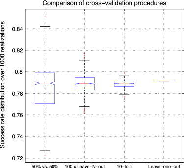
Comparison of cross-validation (CV) procedure for AD vs. CN using hippocampal volumes and subjects' ages in terms of success rate. The 50% vs. 50% CV, 100 × leave-N-out CV, 10-fold CV, and leave-one-out CV were compared using LDA over 1000 realizations. The mean success rates were 78.7%, 78.9%, 79.0%, and 79.1% respectively. The median success rates were 78.9%, 78.9%, 78.9%, and 79.1% respectively.

In practice, alternative validation procedures are used in place of LOOCV for computational reasons when a large number of samples are involved. In the case of the ADNI dataset, the LOOCV required less than 2 seconds and was faster than the 100 × LNOCV. Moreover, LOOCV is known to be an almost unbiased estimator (Cawley and Talbot, 2004). Therefore, we decided to use LOOCV in our validation, since the value obtained with LOOCV corresponds to the median value of the distributions obtained with other CV procedures, without any possible variations in published results according to the random sampling. The maximum values obtained by using 100 × LNOCV and 10-fold CV are presented only for the comparison with previously published work in order to provide the median (i.e., LOOCV) and the upper limit of the success rate distributions for a fairer comparison.

2.4. Implementation details

In this study, we used all the parameters proposed in Coupe et al. (2012a), except for the patch size for EC and the number of training templates used, N. Recently, we showed in Hu et al. (in press) that a patch of 5 × 5 × 5 voxels is sufficient for EC segmentation and is thus used for computational reasons. Here, we used this patch size for EC and patches of 7 × 7 × 7 voxels for HC, as suggested in Coupe et al. (2012a) and Coupe et al. (2011). In Coupe et al. (2012a), we also suggested that 60% of the entire library be selected during template selection (i.e., 30 AD and 30 CN on the 50 available). In this study, we used only around 25% of the entire library (N_AD = 50 and N_CN = 50) for computational reasons. Details on all other parameters can be found in Coupe et al. (2012a)).

3. Results

3.1. SNIPE volumetric study

Fig. 3 shows the volumes obtained by SNIPE for HC and EC. Volumes are plotted according to subject age for the four studied populations, and the distributions are presented as boxplots. We can observe a reduction in the volumes with age for HC, whereas for EC, this reduction is not statistically significant as assessed by p-values and Pearson's coefficients. For HC, a greater reduction can be noted for the AD population, a finding that can be explained by the addition of age-related atrophy to that related to the pathology. The means of the HC volume distributions are significantly different according to a multi-comparison test, and the expected order is observed (AD < pMCI < sMCI < CN). The change in evolution of EC volumes with age is more difficult to interpret. The low Pearson's coefficient r and the high p-values of the linear regressions indicate a nonsignificant linear correlation between EC volumes and age, except for in the AD population. Compared with the results for the HC volumes, this finding might be due to higher intersubject variability and more frequent errors in the segmentation, as discussed in Coupe et al. (2012a). For EC then, the pathology-related patterns seem partially obscured by the intersubject variability. However, except for AD vs. pMCI, the means of EC volume distributions are significantly different according to a multi-comparison test at 95% confidence. Finally, a larger mean difference is observed between sMCI and CN volume distributions than between AD and pMCI (especially for EC volumes).

Fig. 3.

SNIPE-based volumetric study. Left: Volume of HC and EC structures for studied populations according to subject age. Linear regressions are displayed for better visualization of global tendencies. Pearson's coefficients and p-values of the regressions are provided in the legend. Right: Boxplots of the distributions. Colored stars above the boxplots indicate a significantly different mean from those of other groups, obtained using a multi-comparison test at 95% confidence.

3.2. SNIPE grading study

Fig. 4 presents the average grading values obtained by SNIPE for HC and EC. For the studied structures, the grading values are significantly correlated with age (all p-values are < 0.05) and decrease with age. Moreover, this correlation holds when controlling for MMSE. In comparison with those obtained in the volumetric study, the correlation coefficients obtained for grading are higher. As expected, CN subjects have the highest grading values, and AD patients, the lowest. Interestingly, the same observation holds for sMCI compared with pMCI. In all the studied cases, the means of the grading distributions of the studied populations were significantly different. The HC-grade distributions present lower variances and smaller overlap between populations compared with EC-grade distributions. In addition, the boxplots of grade distributions also show fewer outliers (red cross) and a smaller overlap between distributions compared with volume distributions. Finally, as we show later in the classification experiment by comparing volume and grade biomarkers, the higher correlation with age enables a better distinction between anatomical differences due to age-related modifications and those due to pathology-related alterations, and the lower intrapopulation variance enables a better distinction between anatomical differences due to intersubject variability and those due to pathology-related alterations.

Fig. 4.

SNIPE-based grading study. Left: Grade of HC and EC structures for studied populations according to subject age. Linear regressions are displayed for better visualization of global tendencies. Pearson's coefficients and p-values of the regressions are provided in the legend. Right: Boxplots of the distributions. Colored stars above the boxplots indicate a significantly different mean from those for other groups, obtained using a multi-comparison test at 95% confidence.

Visual assessment of the changes in the grading maps with age between populations is proposed in Fig. 5. The estimated scoring is visually lower for AD than for CN. This tendency can also be observed between sMCI and pMCI populations, and a global decrease in grading values with age is visible for the four studied populations. The increased atrophy of HC in the oldest subjects is also visible, especially for pMCI and AD subjects aged 80 to 90 years, in whom the combination of age-related and pathology-related atrophy yields significant HC reduction.

Fig. 5.

Typical grading maps for each population according to subject age.

3.3. Comparison of SNIPE-based biomarkers

Table 2 presents the classification success rates obtained by the imaging biomarkers under consideration for AD vs. CN, pMCI vs. CN, AD vs. sMCI, and pMCI vs. sMCI. These results show that (i) grading-based biomarkers outperform volume-based biomarkers (+ 5% to + 13%) and (ii) EC-based biomarkers are less efficient than HC-based biomarkers, except for AD vs. sMCI where both structures provided similar accuracy. Finally, the combination of volume and grade did not really change results from those obtained with the use of grade only. As assessed by p-values of McNemar test (McNemar, 1947) in Table 2, all the SNIPE-based biomarkers performed significantly better (i.e., p < 0.05) than random classification for all the population comparisons considered. In addition, in order to estimate if the difference between the classification accuracy of biomarkers was significant, we compared the classification results of HC and EC, and of grading and structure volumes in Table 3. By using a confidence interval at 95%, all the biomarkers have significantly different accuracy, except HC-grade > EC-grade for AD vs. sMCI and pMCI vs. sMCI, and HC-vol > EC-vol for pMCI vs. sMCI.

Table 2.

Classification results obtained with different biomarkers for AD vs. CN, pMCI vs. CN, and pMCI vs. sMCI. Results were obtained using linear discriminant analysis through a leave-one-out cross-validation procedure. The values presented in the table correspond to the classification accuracy (acc) in %, the sensitivity (sen) in %, the specificity (spe) in % and the p-value of the McNemar test to assess the performance of classification compared to random classification. For each comparison (e.g., pMCI vs. CN), the best result is in bold and underline.

AD vs. CN	HC acc% / sen%/ spe% (p)	EC acc% / sen%/ spe% (p)	HC-EC acc% / sen%/ spe% (p)
Volume	79 / 76 / 82 (p < 0.0001)	70 / 68 / 72 (p < 0.0001)	78 / 76 / 80 (p < 0.0001)
Grade	88 / 83 / 92 (p < 0.0001)	83 / 75 / 90 (p < 0.0001)	89 / 84 / 93 (p < 0.0001)
Volume + Grade	87 / 83 / 91 (p < 0.0001)	83 / 74 / 91 (p < 0.0001)	88 / 84 / 92 (p < 0.0001)
pMCI vs. CN	HC	EC	HC-EC
Volume	75 / 73 / 76 (p < 0.0001)	69 / 66 / 71 (p < 0.0001)	75 / 74 / 75 (p < 0.0001)
Grade	85 / 80 / 88 (p < 0.0001)	79 / 73 / 83 (p < 0.0001)	86 / 80 / 89 (p < 0.0001)
Volume + Grade	85 / 80 / 88 (p < 0.0001)	80 / 73 / 85 (p < 0.0001)	85 / 80 / 88 (p < 0.0001)
AD vs. sMCI	HC	EC	HC-EC
Volume	68 / 67 / 70 (p < 0.0001)	62 / 57 / 66 (p = 0.0008)	69 / 67 / 70 (p < 0.0001)
Grade	73 / 71 / 75 (p < 0.0001)	72 / 69 / 74 (p < 0.0001)	77 / 77 / 78 (p < 0.0001)
Volume + Grade	73 / 71 / 75 (p < 0.0001)	73 / 70 / 75 (p < 0.0001)	77 / 77 / 77 (p < 0.0001)
pMCI vs. sMCI	HC	EC	HC-EC
Volume	62 / 61 / 63 (p = 0.0007)	59 / 59 / 59 (p = 0.018)	63 / 63 / 64 (p = 0.0003)
Grade	71 / 70 / 71 (p < 0.0001)	66 / 62 / 68 (p < 0.0001)	70 / 69 / 71 (p < 0.0001)
Volume + Grade	71 / 70 / 72 (p < 0.0001)	65 / 60 / 68 (p < 0.0001)	70 / 71 / 69 (p < 0.0001)

Table 3.

Comparison of the classification performance of the different SNIPE-based biomarkers. A McNemar test was used to compare the classification accuracy of EC-based and HC-based biomarkers, and to compare the grading-based and volume-based biomarkers for different populations.

	HC vol > EC vol	HC grad > EC grad	HC grad > HC vol	EC grad > EC vol
AD vs. CN	p = 0.0004	p = 0.0250	p < 0.0001	p < 0.0001
pMCI vs. CN	p = 0.0312	p = 0.0081	p < 0.0001	p = 0.0004
AD vs. sMCI	p = 0.0274	p = 0.6135	p = 0.0360	p = 0.0003
pMCI vs. sMCI	p = 0.2685	p = 0.0648	p = 0.0019	p = 0.0221

As expected, classification accuracies decrease when populations with closer pathological status were used (c.f., Table 2). Thus, the lowest accuracy was obtained for the pMCI vs. sMCI comparison. Although we expected similar results for pMCI vs. CN and AD vs. sMCI, we found an important difference in the classification accuracies of these two comparisons. With SNIPE, a clear difference between the pMCI and CN populations was detected, whereas a less distinctive one was found for AD and sMCI. These classification results seem to show that (i) the pMCI population is relatively similar to the AD population, indicating that the pMCI population studied was advanced in pathology progression and close to conversion, and (ii) the important difference between CN and sMCI may result from anatomical modifications of the HC and EC in these two groups that may be related to the cognitive impairment. Alternatively, it could point to heterogeneity in the sMCI group where some subjects might still convert to pMCI and AD, but not have yet to do so. These subjects may share morphological characteristics with the pMCI group. To investigate these two possibilities further, we analyzed the classification results for AD vs. pMCI and sMCI vs. CN. As shown in Table 4, the detected difference for sMCI vs. CN is clearly greater than that for AD vs. pMCI: the classification of AD vs. pMCI using structure volumes provided results not significantly different to random classification since all p-value are greater than 0.05 while for sMCI vs. CN we obtained a significant difference for these biomarkers.

Table 4.

Classification accuracy obtained for AD vs. pMCI and sMCI vs. CN. Results were obtained using linear discriminant analysis through a leave-one-out cross-validation procedure. The presented results are the classification accuracy (acc) in %, the sensitivity (sen) in %, the specificity (spe) in % and the p-value of the McNemar test to assess the performance of classification compared to random classification. For each comparison the best result is in bold and underline.

AD vs. pMCI	HC acc% / sen%/ spe% (p)	EC acc% / sen%/ spe% (p)	HC-EC acc% / sen%/ spe% (p)
Volume	56 / 51 / 59 (p = 0.163)	51 / 48 / 54 (p = 0.852)	55 / 51 / 58 (p = 0.243)
Grade	58 / 57 / 60 (p = 0.032)	62 / 63 / 60 (p = 0.002)	60 / 60 / 59 (p = 0.012)
Volume + Grade	58 / 57 / 59 (p = 0.039)	61 / 63 / 59 (p = 0.004)	60 / 61 / 59 (p = 0.008)
sMCI vs. CN	HC	EC	HC-EC
Volume	63 / 65 / 62 (p < 0.0001)	60 / 65 / 55 (p = 0.003)	64 / 65 / 63 (p < 0.0001)
Grade	69 / 74 / 63 (p < 0.0001)	63 / 68 / 58 (p < 0.0001)	68 / 76 / 60 (p < 0.0001)
Volume + Grade	69 / 76 / 62 (p < 0.0001)	64 / 72 / 55 (p < 0.0001)	69 / 76 / 63 (p < 0.0001)

For AD vs. CN, our results are in line with the study presented in Coupe et al. (2012a) on 100 baseline scans using QDA, although they were slightly lower for HC and better for EC. The improvement in EC grading might be due to the larger training library used here, which enables a better representation of EC intersubject variability. For AD vs. sMCI, the efficiency of HC grading classification accuracy drops to the level of EC grading (as assessed by p-value in Table 3) and is closer to the accuracy observed for the pMCI vs. sMCI comparison than that for the pMCI vs. CN comparison. For the AD vs. sMCI comparison, HC grade and EC grade seem to be key biomarkers to differentiate between AD and sMCI, whereas for the other population comparisons, HC grade is significantly more efficient (see Table 3). This observation is also confirmed by the results obtained for AD vs. pMCI (see Table 4) where EC grade provided better results than HC grade. This finding may be related to the fact that atrophy of the EC seems to be specific to the pathological processes associated with AD and pMCI, while a linear decrease of HC volume with age has been observed in healthy populations for men starting in the third decade of life, and for women, after menopause (Pruessner et al., 2001). Therefore, for AD vs. sMCI, the advantage of using HC-EC complex grading compared with HC grading is the greatest (+ 4% while around ± 1% for other comparisons, see Table 2). As shown in Coupe et al. (2012a), for AD vs. CN, the combination of HC and EC grade tends to slightly improve classification accuracy. In this study, however, such was not the case for pMCI vs. sMCI. This result was unexpected given that the EC is believed to be affected before the HC in the evolution of the pathology (Frisoni et al., 2010) and thus should be more useful for diagnosis at the early stages of the disease. As previously pointed out, the difficulties related to EC classification (high intersubject variability in shape and size of EC) seem to adversely affect the usefulness of this biomarker for early detection of AD-related pathology.

3.4. Comparison with previous work

Recently, several studies provided extensive comparisons of well-known methods such as methods based on VBM features, methods based on TBM features, CTH, and HC volume applied to the ADNI database (Cuingnet et al., 2011; Wolz et al., 2011b). As a result, estimations of the classification accuracy of different imaging biomarkers can be compared on the same large database. To the best of our knowledge, the study proposed by Wolz et al. (2011b) is currently the most comprehensive work performed on the ADNI database: they used all 834 baseline scans in the ADNI database, studied different scenarios (AD vs. CN, pMCI vs. CN and pMCI vs. sMCI), and they also showed that their method obtained better results than all the methods compared by Cuingnet et al. (2011) (i.e., HC volume, VBM, CTH, and HC shape) on a smaller dataset. Therefore, we chose to compare SNIPE with the results presented in Wolz et al. (2011b) since they represent the best published results for pMCI vs. sMCI, the differentiation of which is the main challenge from a clinical perspective.

We also compared SNIPE with very recent work on sparse representation-based classifiers (SRC) applied to gray matter (GM) and validated in the same AD, pMCI and CN populations (Liu et al., 2012). This SRC approach and SNIPE are based on similar philosophies in that both approaches analyze anatomical similarities using patch comparisons between populations. However, several differences can be pointed out.

• -First, SNIPE uses nonlocal redundancy of information, whereas (Liu et al., 2012) uses local sparsity. The nonlocal/local aspect impacts the anatomy matching of subjects, which in Liu et al. (2012) is achieved by one-to-one mapping after nonlinear registration, whereas SNIPE performs one-to-many mappings after linear registration. The redundancy/sparsity aspect differs in how patches are compared. With redundancy, we try to use the largest possible number of patches to take advantage of the repetition of useful information, thus making a decision based on as much input as possible and minimizing potential errors. By contrast, sparsity aims to find the smallest subset of the most relevant patches.
• -Second, SNIPE focuses on key structures such as the HC and EC, while (Liu et al., 2012) compared the entire GM area. In Liu et al. (2012), a preselection of the ROIs within GM areas is achieved by extracting the most significantly different areas between populations, similarly to what is classically done for CTH.

Tables 5 and 6 show the results of the method comparison between SNIPE using CV procedures proposed in the other two studies.

Table 5.

Comparison of classification results between SNIPE and methods studied in Wolz et al. (2011b). Results shown are the best results obtained using 100 × LNOCV. The presented results are the classification accuracy (acc) in %, the sensitivity (sen) in % and the specificity (spe) in %. Best result for each comparison is in bold and underline.

100× LNOCV	AD vs. CN acc%/sen%/spe%	pMCI vs. CN acc%/sen%/spe%	pMCI vs. sMCI acc%/sen%/spe%
SNIPE
•HC Volume	83 / 80 / 85	78 / 77 / 78	66 / 65 / 67
•HC Grade	90 / 86 / 93	87 / 83 / 90	74 / 73 / 74
•HC-EC Volume	80 / 80 / 81	78 / 78 / 77	67 / 66 / 68
•HC-EC Grade	91 / 87 / 94	88 / 83 / 91	73 / 72 / 74
Multi-Method (Wolz et al., 2011b)
•HC Volume	81 / 81 / 79	76 / 77 / 76	65 / 63 / 67
•Manifold-based learning	85 / 87 / 83	78 / 81 / 75	65 / 64 / 66
•Cortical thickness	81 / 89 / 71	77 / 85 / 65	56 / 63 / 45
•Tensor-based method	87 / 90 / 84	79 / 82 / 76	64 / 65 / 62
•All	89 / 93 / 85	84 / 86 / 82	68 / 67 / 69

Table 6.

Comparison of classification results between SNIPE and methods studied in Liu et al. (2012). Results shown are the best results obtained using 10-fold CV. The presented results are the classification accuracy in %, the sensitivity in % and the specificity in %. Best result for each comparison is in bold and underline.

10-Fold CV	AD vs. CN acc%/sen%/spe%	pMCI vs. CN acc%/sen%/spe%	pMCI vs. sMCI acc%/sen%/spe%
SNIPE
•HC Volume	83 / 80 / 86	80 / 79 / 80	66 / 67 / 65
•HC Grade	90 / 85 / 94	87 / 85 / 89	71 / 70 / 71
•HC-EC Volume	83 / 82 / 84	80 / 78 / 81	68 / 64 / 71
•HC-EC Grade	90 / 85 / 94	87 / 83 / 90	73 / 68 / 76
Sparse Classification (Liu et al., 2012)
•COMPARE	81 / 79 / 83	–	–
•Global SVM	85 / 73 / 95	81 / 73 / 90	–
•Global SRC	88 / 81 / 94	85 / 83 / 87	–
•Patch-based SVM	86 / 75 / 94	82 / 74 / 91	–
•Patch-based SRC	91 / 86 / 95	88 / 85 / 90	–

For AD vs. CN, the results obtained with SNIPE were similar to those from the combination of four methods reported in Wolz et al. (2011b) (91% compared to 89% using 100 × LNOCV, see Table 5). SNIPE obtained better results than HC volume (Lotjonen et al., 2011), manifold-based learning (Wolz et al., 2011a), CTH (Lerch and Evans, 2005), and method based on TBM features (Koikkalainen et al., 2011), although the results from multi-template TBM and SNIPE were close, as were those from SNIPE and patch-based SRC (Liu et al., 2012) (90% compared to 91% using k-fold CV, see Table 6). The results obtained for HC volumes using patch-based segmentation (Coupe et al., 2011) and multi-template nonlinear warping (Lotjonen et al., 2011) were also close (83% compared to 81% using 100 × LNOCV, see Table 5). These findings seem to indicate that the compared approaches provide similar segmentation accuracies. Interestingly, HC grade provided results that were similar to or better than those from methods analyzing the entire brain anatomy (i.e., method based on TBM features, global SVM/SRC, and advanced method based on VBM features such as COMPARE (Fan et al., 2007)) and requiring nonlinear registration of all subjects.

For pMCI vs. CN, the results obtained by SNIPE were similar to those from patch-based SRC (87% compared to 88% using k-fold CV, see Table 6) but better than those from all the methods compared in Wolz et al. (2011b) as well as their combination (88% compared to 84% using 100 × LNOCV, see Table 5). This finding seems to indicate that new patch-based frameworks perform better than classical methods such as HC volume or methods based on TBM features. In addition, preselecting the most relevant GM areas or using segmentation of key structures seems to lead to similar classification accuracy. The latter has the advantage of directly avoiding double-dipping.

For pMCI vs. sMCI, the results obtained by SNIPE were better than those from all the methods compared in Wolz et al. (2011b) (74% compared to 68% using 100 × LNOCV, see Table 5). This outcome highlights the potential of SNIPE for AD prediction by enabling the detection of subtle anatomical changes caused by AD at the early stages of the pathology. Unfortunately, Liu et al. (2012) did not provide results for this comparison, and thus no comparison between efficiency of redundancy and sparsity can be done for early detection.

3.5. Patch-based morphometry analysis

Another important aspect of a method is its potential to visualize the differences between populations in a compact way. This capability is one explanation for the great success of the VBM, CTH, and TBM methods. In their discussion, Liu et al. (2012) warn that the main limitation of their method is the impossibility of visualizing the spatial location of the most discriminant areas between populations. They conclude that this limitation results in less clinical insight and thus a lower understanding of the pathology mechanisms.

Recently, we proposed a new patch-based morphometry (PBM) method based on SNIPE to study anatomical differences between AD and CN in the entire brain (Coupe et al., 2012b). Instead of comparing tissue probability as done in voxel-based morphometry, PBM compares grading maps. Therefore the comparison between populations is based on the score assigned to a voxel according to the similarity of its surrounding patch with the patch libraries derived from both populations. Here, we propose a similar approach but for studying the typical spatial distribution of grade for each population over the entire ADNI database. First, the grading maps were warped to our population-specific template derived from the ADNI database and constructed using the algorithm published in Fonov et al. (2011) with ANIMAL non-linear registration (Collins and Evans, 1997). To do that, each subject's T1w MRI was nonlinearly registered onto our template. The resulting transformation was then applied to the subject's grading maps. Finally, a mean grading map was estimated, voxel-by-voxel, for each population using the nonlinearly warped maps. This way, the spatial distribution of grading values was obtained for each population studied to enable a compact visualization of population differences.

Fig. 6 shows the mean grading maps obtained for CN, sMCI, pMCI, and AD populations. A clear difference can be observed between each of the populations, especially at the HC level. At the global level, the PBM results indicate that the posterior part of the HC seems to be the location of major differences between sMCI and pMCI while the main difference detected between AD and CN seems to be observed at the body and head level of the HC (i.e., anterior part). In addition, the right HC seems to be more discriminant between CN and sMCI, while the left HC shows a greater difference between pMCI and AD. This might indicate that the right HC is first impacted by AD pathology.

Fig. 6.

Mean grading map for each population overlaid on our population-specific template derived from the subset of the ADNI database. These mean grading maps were obtained by first nonlinearly registering all the grading maps of the ADNI database to our population-specific template. Then, the warped grading maps were averaged according to the population. The grading values are displayed with the same range [− 0.15, 0.15] for the four populations. The values above 0.15 are set display in white and the values under − 0.15 are displayed in black.

4. Discussion

In this study, we showed that SNIPE-based grading biomarkers provided competitive results for early detection of AD compared with conventional methods such as HC volume, CTH, and method based on TBM features. We also found that new patch-based paradigms (nonlocal redundancy and local sparsity) are promising ways of detecting subtle anatomical changes between populations. Further investigations into these new approaches are still required to determine the best direction for future study. First, the scale of analysis needs intensive study (i.e., key structures vs. whole brain). In future work, we hope to analyze the grading of the whole GM area in order to shed some light on this point. In addition, the optimal way of comparing patches (i.e., redundancy vs. sparsity) should be more carefully studied by using a similar framework for training library construction (i.e., local vs. nonlocal). In recent denoising literature (Mairal et al., 2009; Manjon et al., 2012), sparsity-based filters seem to provide slightly better results than nonlocal means filters. We believe that a nonlocal sparsity approach may be a promising way of achieving this type of scoring, as the well-defined one-to-many correspondence would be coupled with the efficiency of a sparse-based approach.

We also discussed the issue of the cross-validation procedure, highlighting that LOOCV is a good option because the published results can be compared without any variation due to the random splitting of populations. Our experiment showed that, for the ADNI database, LOOCV provided an estimate similar to the mean/median of the compared CV. Therefore; we used an LOOCV procedure for the comparison of SNIPE-based biomarkers. The discussion on bias during validation complements our recent discussion on double-dipping issues presented in Eskildsen et al. (in press). Both the variation in success rates due to CV and the overestimation of success rates rate due to double-dipping should be considered in future studies in order to limit their impact on published results.

The comparison of SNIPE-based biomarkers in the context of early detection demonstrated the high potential of the proposed framework for this key clinical problem. Although the prediction rate obtained (71% with LOOCV, 73% with 10-fold CV and 74% with 100 × LNOCV) is not yet suitable for clinical use, the recent progress of MRI-based biomarkers on this challenging classification problem is encouraging. In fact, still very recently, the highest success rate was only around 56% on the ADNI database (Davatzikos et al., 2011) using advanced VBM-like analysis such as Spatial Pattern of Abnormalities for Recognition of Early AD (SPARSE-AD) (Misra et al., 2009). It is also encouraging to note that the improvements brought by SNIPE were not obtained at the expense of method or computational complexity. SNIPE requires only linear registration and can be implemented easily. In addition, its computational time is around 5 minutes per subject using CPU implementation, and this time can be further reduced by using GPU implementations, as already proposed for real-time processing in denoising literature (Palhano Xavier de Fontes et al., 2011). In the case where the computational cost is not a limiting factor, variants of SNIPE based on nonlinear registration might be used by involving local or semi-local label fusion methods (Sabuncu et al., 2010; Wang et al., 2011) after nonlinear registration of all the subjects. This would result in a method similar to the sparse-based method (Liu et al., 2012) mentioned in this paper. The combination of nonlocal patch-based method with nonlinear registration has been recently proposed for segmentation (Fonov et al., 2012). Finally, the simplicity of the SNIPE framework results in a robust pipeline; the processing failure rate was less than 1.7% at the linear registration step—a much lower failure rate in great contrast to the 13% obtained for the CTH method presented in Wolz et al. (2011b).

The last part of this study was dedicated to the analysis of pathology progression using patch-based morphometry (PBM) (Coupe et al., 2012b). With this new approach, we were able to present the mean grading map for each population. Global PBM results seem to indicate that the anterior part of the HC (i.e., head and anterior body) is the more discriminant area between AD and CN populations. More interestingly, the first alterations of the HC seem to be located in the posterior part (i.e., tail and posterior body). In further work, our PBM results should be analyzed using HC subfields atlas as already done in literature using HC shape analysis (Apostolova et al., 2006; Frisoni et al., 2008; Gerardin et al., 2009) or volumetric approaches (Atienza et al., 2011; Hanseeuw et al., 2011; Mueller et al., 2010). This type of HC subfields analysis should enable a comparison of our findings with current knowledge about AD progression derived from histological studies (Lace et al., 2009; Schonheit et al., 2004).

5. Conclusion

This study analyzed the capability of SNIPE to perform early detection of AD. The experiments were carried out on the entire ADNI database (834 subjects). A comparison with recent methods proposed for the crucial problem of AD prediction highlights the competitive results obtained by SNIPE-based biomarkers. In addition, the first results of patch-based morphometry analysis were presented as a new way of studying pathology progression. Finally, a discussion was provided on the promising results proposed by new patch-based frameworks based on redundancy and sparsity.

References

- Aizenstein H.J., Nebes R.D., Saxton J.A., Price J.C., Mathis C.A., Tsopelas N.D., Ziolko S.K., James J.A., Snitz B.E., Houck P.R., Bi W., Cohen A.D., Lopresti B.J., DeKosky S.T., Halligan E.M., Klunk W.E. Frequent amyloid deposition without significant cognitive impairment among the elderly. Archives of Neurology. 2008;65:1509–1517. doi: 10.1001/archneur.65.11.1509. [DOI] [PMC free article] [PubMed] [Google Scholar]
- Amieva H., Le Goff M., Millet X., Orgogozo J.M., Peres K., Barberger-Gateau P., Jacqmin-Gadda H., Dartigues J.F. Prodromal Alzheimer's disease: successive emergence of the clinical symptoms. Annals of Neurology. 2008;64:492–498. doi: 10.1002/ana.21509. [DOI] [PubMed] [Google Scholar]
- Apostolova L.G., Dinov I.D., Dutton R.A., Hayashi K.M., Toga A.W., Cummings J.L., Thompson P.M. 3D comparison of hippocampal atrophy in amnestic mild cognitive impairment and Alzheimer's disease. Brain : A Journal of Neurology. 2006;129:2867–2873. doi: 10.1093/brain/awl274. [DOI] [PubMed] [Google Scholar]
- Ashburner J., Friston K.J. Voxel-based morphometry—the methods. NeuroImage. 2000;11:805–821. doi: 10.1006/nimg.2000.0582. [DOI] [PubMed] [Google Scholar]
- Atienza M., Atalaia-Silva K.C., Gonzalez-Escamilla G., Gil-Neciga E., Suarez-Gonzalez A., Cantero J.L. Associative memory deficits in mild cognitive impairment: the role of hippocampal formation. NeuroImage. 2011;57:1331–1342. doi: 10.1016/j.neuroimage.2011.05.047. [DOI] [PubMed] [Google Scholar]
- Ballard C., Khan Z., Clack H., Corbett A. Nonpharmacological treatment of Alzheimer disease. Canadian Journal of Psychiatry. Revue Canadienne de Psychiatrie. 2011;56:589–595. doi: 10.1177/070674371105601004. [DOI] [PubMed] [Google Scholar]
- Braak H., Braak E. Neuropathological stageing of Alzheimer-related changes. Acta Neuropathologica. 1991;82:239–259. doi: 10.1007/BF00308809. [DOI] [PubMed] [Google Scholar]
- Cawley G.C., Talbot N.L. Fast exact leave-one-out cross-validation of sparse least-squares support vector machines. Neural Networks : The Official Journal of the International Neural Network Society. 2004;17:1467–1475. doi: 10.1016/j.neunet.2004.07.002. [DOI] [PubMed] [Google Scholar]
- Chetelat G., Villemagne V.L., Bourgeat P., Pike K.E., Jones G., Ames D., Ellis K.A., Szoeke C., Martins R.N., O'Keefe G.J., Salvado O., Masters C.L., Rowe C.C. Relationship between atrophy and beta-amyloid deposition in Alzheimer disease. Annals of Neurology. 2010;67:317–324. doi: 10.1002/ana.21955. [DOI] [PubMed] [Google Scholar]
- Cho Y., Seong J.K., Jeong Y., Shin S.Y. Individual subject classification for Alzheimer's disease based on incremental learning using a spatial frequency representation of cortical thickness data. NeuroImage. 2012;59:2217–2230. doi: 10.1016/j.neuroimage.2011.09.085. [DOI] [PMC free article] [PubMed] [Google Scholar]
- Chupin M., Gerardin E., Cuingnet R., Boutet C., Lemieux L., Lehericy S., Benali H., Garnero L., Colliot O. Fully automatic hippocampus segmentation and classification in Alzheimer's disease and mild cognitive impairment applied on data from ADNI. Hippocampus. 2009;19:579–587. doi: 10.1002/hipo.20626. [DOI] [PMC free article] [PubMed] [Google Scholar]
- Collins D.L., Evans A.C. Animal: validation and applications of nonlinear registration-based segmentation. International Journal of Pattern Recognition and Artificial Intelligence. 1997;11:1271–1294. [Google Scholar]
- Collins D.L., Neelin P., Peters T.M., Evans A.C. Automatic 3D intersubject registration of MR volumetric data in standardized Talairach space. Journal of Computer Assisted Tomography. 1994;18:192–205. [PubMed] [Google Scholar]
- Coupe P., Yger P., Prima S., Hellier P., Kervrann C., Barillot C. An optimized blockwise nonlocal means denoising filter for 3-D magnetic resonance images. IEEE Transactions on Medical Imaging. 2008;27:425–441. doi: 10.1109/TMI.2007.906087. [DOI] [PMC free article] [PubMed] [Google Scholar]
- Coupe P., Manjon J.V., Gedamu E., Arnold D., Robles M., Collins D.L. Robust Rician noise estimation for MR images. Medical Image Analysis. 2010;14:483–493. doi: 10.1016/j.media.2010.03.001. [DOI] [PubMed] [Google Scholar]
- Coupe P., Manjon J.V., Fonov V., Pruessner J., Robles M., Collins D.L. Patch-based segmentation using expert priors: application to hippocampus and ventricle segmentation. NeuroImage. 2011;54:940–954. doi: 10.1016/j.neuroimage.2010.09.018. [DOI] [PubMed] [Google Scholar]
- Coupe P., Eskildsen S.F., Manjon J.V., Fonov V.S., Collins D.L. Simultaneous segmentation and grading of anatomical structures for patient's classification: application to Alzheimer's disease. NeuroImage. 2012;59:3736–3747. doi: 10.1016/j.neuroimage.2011.10.080. [DOI] [PubMed] [Google Scholar]
- Coupe P., Manjon J., Fonov V.S., Eskildsen S.F., Collins D.L., ADNI . Alzheimer's Association International Conference. 2012. Patch-based morphometry: application to Alzheimer's Disease. [Google Scholar]
- Cuingnet R., Gerardin E., Tessieras J., Auzias G., Lehericy S., Habert M.O., Chupin M., Benali H., Colliot O. Automatic classification of patients with Alzheimer's disease from structural MRI: a comparison of ten methods using the ADNI database. NeuroImage. 2011;56:766–781. doi: 10.1016/j.neuroimage.2010.06.013. [DOI] [PubMed] [Google Scholar]
- Davatzikos C., Bhatt P., Shaw L.M., Batmanghelich K.N., Trojanowski J.Q. Prediction of MCI to AD conversion, via MRI, CSF biomarkers, and pattern classification. Neurobiology of Aging. 2011;32(2322):e2319–e2327. doi: 10.1016/j.neurobiolaging.2010.05.023. [DOI] [PMC free article] [PubMed] [Google Scholar]
- de Jong L.W., van der Hiele K., Veer I.M., Houwing J.J., Westendorp R.G., Bollen E.L., de Bruin P.W., Middelkoop H.A., van Buchem M.A., van der Grond J. Strongly reduced volumes of putamen and thalamus in Alzheimer's disease: an MRI study. Brain : A Journal of Neurology. 2008;131:3277–3285. doi: 10.1093/brain/awn278. [DOI] [PMC free article] [PubMed] [Google Scholar]
- Du A.T., Schuff N., Amend D., Laakso M.P., Hsu Y.Y., Jagust W.J., Yaffe K., Kramer J.H., Reed B., Norman D., Chui H.C., Weiner M.W. Magnetic resonance imaging of the entorhinal cortex and hippocampus in mild cognitive impairment and Alzheimer's disease. Journal of Neurology, Neurosurgery, and Psychiatry. 2001;71:441–447. doi: 10.1136/jnnp.71.4.441. [DOI] [PMC free article] [PubMed] [Google Scholar]
- Elias M.F., Beiser A., Wolf P.A., Au R., White R.F., D'Agostino R.B. The preclinical phase of Alzheimer disease: a 22-year prospective study of the Framingham Cohort. Archives of Neurology. 2000;57:808–813. doi: 10.1001/archneur.57.6.808. [DOI] [PubMed] [Google Scholar]
- Eskildsen S.F., Coupe P., Fonov V., Manjon J.V., Leung K.K., Guizard N., Wassef S.N., Ostergaard L.R., Collins D.L. BEaST: brain extraction based on nonlocal segmentation technique. NeuroImage. 2012;59:2362–2373. doi: 10.1016/j.neuroimage.2011.09.012. [DOI] [PubMed] [Google Scholar]
- Eskildsen, S.F., Coupé, P., García-Lorenzo, D., Fonov, V., Pruessner, J.C., Collins, D.L., The Alzheimer's Disease Neuroimaging Initiative, in press. Prediction of Alzheimer's disease in subjects with mild cognitive impairment from the ADNI cohort using patterns of cortical thinning. Neuroimage. pii: S1053-8119(12)00975-5. http://dx.doi.org/10.1016/j.neuroimage.2012.09.058 (2012 Oct 2, Epub ahead of print). [DOI] [PMC free article] [PubMed]
- Fan Y., Shen D., Gur R.C., Gur R.E., Davatzikos C. COMPARE: classification of morphological patterns using adaptive regional elements. IEEE Transactions on Medical Imaging. 2007;26:93–105. doi: 10.1109/TMI.2006.886812. [DOI] [PubMed] [Google Scholar]
- Fonov V., Evans A.C., Botteron K., Almli C.R., McKinstry R.C., Collins D.L. Unbiased average age-appropriate atlases for pediatric studies. NeuroImage. 2011;54:313–327. doi: 10.1016/j.neuroimage.2010.07.033. [DOI] [PMC free article] [PubMed] [Google Scholar]
- Fonov V., Coupé P., Styner M., Collins D. Annual Meeting of the Organization for Human Brain Mapping. Beijing, China; 2012. Automatic lateral ventricle segmentation in infant population with high risk of autism. [Google Scholar]
- Frisoni G.B., Ganzola R., Canu E., Rub U., Pizzini F.B., Alessandrini F., Zoccatelli G., Beltramello A., Caltagirone C., Thompson P.M. Mapping local hippocampal changes in Alzheimer's disease and normal ageing with MRI at 3 Tesla. Brain : A Journal of Neurology. 2008;131:3266–3276. doi: 10.1093/brain/awn280. [DOI] [PubMed] [Google Scholar]
- Frisoni G.B., Fox N.C., Jack C.R., Scheltens P., Thompson P.M. The clinical use of structural MRI in Alzheimer disease. Nature Reviews. Neurology. 2010;6:67–77. doi: 10.1038/nrneurol.2009.215. [DOI] [PMC free article] [PubMed] [Google Scholar]
- Gerardin E., Chetelat G., Chupin M., Cuingnet R., Desgranges B., Kim H.S., Niethammer M., Dubois B., Lehericy S., Garnero L., Eustache F., Colliot O. Multidimensional classification of hippocampal shape features discriminates Alzheimer's disease and mild cognitive impairment from normal aging. NeuroImage. 2009;47:1476–1486. doi: 10.1016/j.neuroimage.2009.05.036. [DOI] [PMC free article] [PubMed] [Google Scholar]
- Hanseeuw B.J., Van Leemput K., Kavec M., Grandin C., Seron X., Ivanoiu A. Mild cognitive impairment: differential atrophy in the hippocampal subfields. AJNR. American Journal of Neuroradiology. 2011;32:1658–1661. doi: 10.3174/ajnr.A2589. [DOI] [PMC free article] [PubMed] [Google Scholar]
- Hu, S., Coupé, P., Pruessner, J.C., Collins, D.L., in press. Nonlocal regularization for active appearance model: application to medial temporal lobe segmentation. Human Brain Mapping. http://dx.doi.org/10.1002/hbm.22183 [2012 Sep 15, Epub ahead of print]. [DOI] [PMC free article] [PubMed]
- Kantarci K., Yang C., Schneider J.A., Senjem M.L., Reyes D.A., Lowe V.J., Barnes L.L., Aggarwal N.T., Bennett D.A., Smith G.E., Petersen R.C., Jack C.R., Jr., Boeve B.F. Ante mortem amyloid imaging and beta-amyloid pathology in a case with dementia with Lewy bodies. Neurobiology of Aging. 2012;33:878–885. doi: 10.1016/j.neurobiolaging.2010.08.007. [DOI] [PMC free article] [PubMed] [Google Scholar]
- Kloppel S., Stonnington C.M., Chu C., Draganski B., Scahill R.I., Rohrer J.D., Fox N.C., Jack C.R., Jr., Ashburner J., Frackowiak R.S. Automatic classification of MR scans in Alzheimer's disease. Brain : A Journal of Neurology. 2008;131:681–689. doi: 10.1093/brain/awm319. [DOI] [PMC free article] [PubMed] [Google Scholar]
- Koikkalainen J., Lotjonen J., Thurfjell L., Rueckert D., Waldemar G., Soininen H. Multi-template tensor-based morphometry: application to analysis of Alzheimer's disease. NeuroImage. 2011;56:1134–1144. doi: 10.1016/j.neuroimage.2011.03.029. [DOI] [PMC free article] [PubMed] [Google Scholar]
- Kriegeskorte N., Simmons W.K., Bellgowan P.S., Baker C.I. Circular analysis in systems neuroscience: the dangers of double dipping. Nature Neuroscience. 2009;12:535–540. doi: 10.1038/nn.2303. [DOI] [PMC free article] [PubMed] [Google Scholar]
- Lace G., Savva G.M., Forster G., de Silva R., Brayne C., Matthews F.E., Barclay J.J., Dakin L., Ince P.G., Wharton S.B. Hippocampal tau pathology is related to neuroanatomical connections: an ageing population-based study. Brain : A Journal of Neurology. 2009;132:1324–1334. doi: 10.1093/brain/awp059. [DOI] [PubMed] [Google Scholar]
- Lerch J.P., Evans A.C. Cortical thickness analysis examined through power analysis and a population simulation. NeuroImage. 2005;24:163–173. doi: 10.1016/j.neuroimage.2004.07.045. [DOI] [PubMed] [Google Scholar]
- Liu M., Zhang D., Shen D. Ensemble sparse classification of Alzheimer's disease. NeuroImage. 2012;60:1106–1116. doi: 10.1016/j.neuroimage.2012.01.055. [DOI] [PMC free article] [PubMed] [Google Scholar]
- Lotjonen J., Wolz R., Koikkalainen J., Julkunen V., Thurfjell L., Lundqvist R., Waldemar G., Soininen H., Rueckert D. Fast and robust extraction of hippocampus from MR images for diagnostics of Alzheimer's disease. NeuroImage. 2011;56:185–196. doi: 10.1016/j.neuroimage.2011.01.062. [DOI] [PMC free article] [PubMed] [Google Scholar]
- Mairal J., Bach F., Ponce J., Sapiro G., Zisserman A. Computer Vision, 2009 IEEE 12th International Conference on. 2009. Non-local sparse models for image restoration; pp. 2272–2279. [Google Scholar]
- Manjon J.V., Coupe P., Buades A., Louis Collins D., Robles M. New methods for MRI denoising based on sparseness and self-similarity. Medical Image Analysis. 2012;16:18–27. doi: 10.1016/j.media.2011.04.003. [DOI] [PubMed] [Google Scholar]
- McNemar Q. Note on the sampling error of the difference between correlated proportions or percentages. Psychometrika. 1947;12:153–157. doi: 10.1007/BF02295996. [DOI] [PubMed] [Google Scholar]
- Misra C., Fan Y., Davatzikos C. Baseline and longitudinal patterns of brain atrophy in MCI patients, and their use in prediction of short-term conversion to AD: results from ADNI. NeuroImage. 2009;44:1415–1422. doi: 10.1016/j.neuroimage.2008.10.031. [DOI] [PMC free article] [PubMed] [Google Scholar]
- Mueller S.G., Schuff N., Yaffe K., Madison C., Miller B., Weiner M.W. Hippocampal atrophy patterns in mild cognitive impairment and Alzheimer's disease. Human Brain Mapping. 2010;31:1339–1347. doi: 10.1002/hbm.20934. [DOI] [PMC free article] [PubMed] [Google Scholar]
- Nyul L.G., Udupa J.K. Vol. 1. 2000. Standardizing the MR image intensity scales: making MR intensities have tissue specific meaning; pp. 496–504. (Medical Imaging 2000: Image Display and Visualization). [Google Scholar]
- Palhano Xavier de Fontes F., Andrade Barroso G., Coupé P., Hellier P. Real time ultrasound image denoising. Journal of Real-Time Image Processing. 2011;6(1):15–22. [Google Scholar]
- Pruessner J.C., Collins D.L., Pruessner M., Evans A.C. Age and gender predict volume decline in the anterior and posterior hippocampus in early adulthood. J Neurosci. 2001;21(1):194–200. doi: 10.1523/JNEUROSCI.21-01-00194.2001. (Jan 1) [DOI] [PMC free article] [PubMed] [Google Scholar]
- Pruessner J.C., Kohler S., Crane J., Pruessner M., Lord C., Byrne A., Kabani N., Collins D.L., Evans A.C. Volumetry of temporopolar, perirhinal, entorhinal and parahippocampal cortex from high-resolution MR images: considering the variability of the collateral sulcus. Cerebral Cortex. 2002;12:1342–1353. doi: 10.1093/cercor/12.12.1342. [DOI] [PubMed] [Google Scholar]
- Querbes O., Aubry F., Pariente J., Lotterie J.A., Demonet J.F., Duret V., Puel M., Berry I., Fort J.C., Celsis P. Early diagnosis of Alzheimer's disease using cortical thickness: impact of cognitive reserve. Brain : A Journal of Neurology. 2009;132:2036–2047. doi: 10.1093/brain/awp105. [DOI] [PMC free article] [PubMed] [Google Scholar]
- Sabuncu M.R., Yeo B.T., Van Leemput K., Fischl B., Golland P. A generative model for image segmentation based on label fusion. IEEE Transactions on Medical Imaging. 2010;29:1714–1729. doi: 10.1109/TMI.2010.2050897. [DOI] [PMC free article] [PubMed] [Google Scholar]
- Schonheit B., Zarski R., Ohm T.G. Spatial and temporal relationships between plaques and tangles in Alzheimer-pathology. Neurobiology of Aging. 2004;25:697–711. doi: 10.1016/j.neurobiolaging.2003.09.009. [DOI] [PubMed] [Google Scholar]
- Sled J.G., Zijdenbos A.P., Evans A.C. A nonparametric method for automatic correction of intensity nonuniformity in MRI data. IEEE Transactions on Medical Imaging. 1998;17:87–97. doi: 10.1109/42.668698. [DOI] [PubMed] [Google Scholar]
- Vemuri P., Gunter J.L., Senjem M.L., Whitwell J.L., Kantarci K., Knopman D.S., Boeve B.F., Petersen R.C., Jack C.R., Jr. Alzheimer's disease diagnosis in individual subjects using structural MR images: validation studies. NeuroImage. 2008;39:1186–1197. doi: 10.1016/j.neuroimage.2007.09.073. [DOI] [PMC free article] [PubMed] [Google Scholar]
- Villemagne V.L., Pike K.E., Chetelat G., Ellis K.A., Mulligan R.S., Bourgeat P., Ackermann U., Jones G., Szoeke C., Salvado O., Martins R., O'Keefe G., Mathis C.A., Klunk W.E., Ames D., Masters C.L., Rowe C.C. Longitudinal assessment of Abeta and cognition in aging and Alzheimer disease. Annals of Neurology. 2011;69:181–192. doi: 10.1002/ana.22248. [DOI] [PMC free article] [PubMed] [Google Scholar]
- Wang H., Das S.R., Suh J.W., Altinay M., Pluta J., Craige C., Avants B., Yushkevich P.A. A learning-based wrapper method to correct systematic errors in automatic image segmentation: consistently improved performance in hippocampus, cortex and brain segmentation. NeuroImage. 2011;55:968–985. doi: 10.1016/j.neuroimage.2011.01.006. [DOI] [PMC free article] [PubMed] [Google Scholar]
- Westman E., Simmons A., Muehlboeck J.S., Mecocci P., Vellas B., Tsolaki M., Kloszewska I., Soininen H., Weiner M.W., Lovestone S., Spenger C., Wahlund L.O. AddNeuroMed and ADNI: similar patterns of Alzheimer's atrophy and automated MRI classification accuracy in Europe and North America. NeuroImage. 2011;58:818–828. doi: 10.1016/j.neuroimage.2011.06.065. [DOI] [PubMed] [Google Scholar]
- Wolz R., Aljabar P., Hajnal J.V., Lotjonen J., Rueckert D. Biomedical Imaging: From Nano to Macro, 2011 IEEE International Symposium on. 2011. Manifold learning combining imaging with non-imaging information; pp. 1637–1640. [Google Scholar]
- Wolz R., Julkunen V., Koikkalainen J., Niskanen E., Zhang D.P., Rueckert D., Soininen H., Lotjonen J. Multi-method analysis of MRI images in early diagnostics of Alzheimer's disease. PLoS One. 2011;6:e25446. doi: 10.1371/journal.pone.0025446. [DOI] [PMC free article] [PubMed] [Google Scholar]