Honest signalling with costly gambles

Abstract

Costly signalling theory is commonly invoked as an explanation for how honest communication can be stable when interests conflict. However, the signal costs predicted by costly signalling models often turn out to be unrealistically high. These models generally assume that signal cost is determinate. Here, we consider the case where signal cost is instead stochastic. We examine both discrete and continuous signalling games and show that, under reasonable assumptions, stochasticity in signal costs can decrease the average cost at equilibrium for all individuals. This effect of stochasticity for decreasing signal costs is a fundamental mechanism that probably acts in a wide variety of circumstances.

1. Introduction

Signalling and communication abound in nature and human society [1]. Often, communication takes place between entities that do not share entirely coincident interests. Yet, honest communication frequently persists in spite of incentives to deceive. Evolutionary biologists and economists alike have developed a suite of game-theoretic models that aim to explain how communication can originate and be maintained among individuals with partially conflicting interests [2,3]. Biologists have paid particular attention to the role of signal cost in stabilizing communication [4]. Costly signalling models propose that appropriate signal costs can facilitate honest communication by making deceptive signals so expensive that they become counterproductive. While this class of signalling models allows communication at equilibrium, honesty often comes at considerable cost. Signal costs can be so high that all participants in a costly signalling interaction end up worse off at the signalling equilibrium than in an alternative equilibrium in which no communication takes place [5]. For this reason, there has been considerable interest in understanding how honest signalling can occur without high cost. Researchers have noted that honest signals need not be costly so long as dishonest signals are expensive [6–9] and proposed that mechanisms such as punishment or spatial structure can further reduce signal costs while allowing honesty to persist [10–16]. These analyses have generally assumed determinate signal costs. In this paper, we study signalling models with stochastic costs and show that this simple difference can have substantial consequences for individuals in terms of their average costs at equilibrium.

We examine a type of action–response game where a signaller with private information may send a signal to a receiver who must then select a response. Sending a signal carries a cost, which depends on the condition of the signaller. We study the case when this cost is a random variable, and characterize how the average costs at equilibrium depend on the risk preferences of signallers. We show that, when signallers have decreasing absolute risk aversion (DARA; defined in the following section), stochasticity facilitates honest communication at lower expected cost. We present two models: a discrete action–response game with two signaller qualities, two signals and two responses, and a continuous signalling game with a continuum of qualities, signals and responses.

2. Measures of risk preferences

To study the relative costliness of signals that involve risk, we must know how an individual's welfare depends on the risk taken. In a biological context, this means we must know how the resource being risked translates into reproductive success or fitness. Many types of resources exhibit diminishing returns. That is, a needy individual's fitness will increase more than a well-off individual's fitness if they both obtain the same amount of additional resources. In an economic context, this is the same as saying that individuals have concave utility functions—or equivalently that they are risk averse. An example of such a function is illustrated in figure 1. In the economic context, utility is the analogue of fitness and wealth is the resource of interest. We present our models within an economic framework because economics provides a well-developed theory of risk and precise terminology. However, the models we present are general, and we interpret the implications of our results for biological contexts as well as economic ones.

Figure 1.

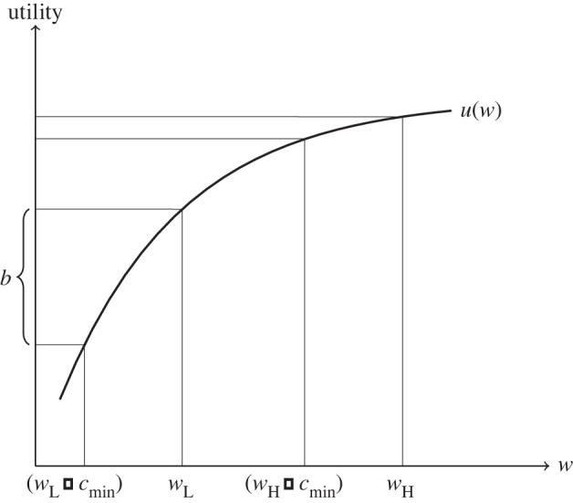
The signaller has a concave utility function u(w). The benefit of being accepted by the signal receiver is a utility increment of magnitude b. The minimal cost for stable honest signalling is c_min.

With the above points in mind, we describe some economic terminology for risk preferences. Any statement about the risk preferences of an individual can be translated into a statement about the shape of her utility function, u. If an individual prefers a sure thing of getting $10 to a bet that has an expected pay-off of $10, that is the individual is risk averse, this is equivalent to saying that the second derivative of u is negative. If an individual is less willing to risk $10 when poor than when rich, then her utility function exhibits DARA. The geometric equivalent is that −u″/u′ is decreasing. The assumption of DARA is standard in economics and is supported by empirical studies in humans [17]. In the biological context, assuming DARA means that the fitness consequences of risking resources are more grave when resources are rare. The extent to which this is the norm in nature is an empirical question, but it would be surprising if having more resources did not often put an individual in a position to be more willing to risk some of them.

3. Discrete model

In order to understand how risk influences costly signalling, we will compare two signalling games, one in which the signals involve risk and one in which they do not.

3.1. Deterministic signalling

We first establish the baseline for comparison: a standard costly signalling game in which individuals signal their wealth by deterministically burning some portion of that wealth. We assume that our signallers have a utility function u(·) that is increasing but concave in wealth, as in figure 1. (Within the economic framework, this utility is conceptualized as von Neumann–Morgenstern utility.)

Our base discrete action–response game is illustrated in figure 2. The signaller may be in one of two conditions: high, with a high wealth w_H, or low, with a low wealth w_L. The signaller chooses whether or not to send a costly signal by squandering a pre-set amount of money c on a costly signal with no value beyond its communicative role (imagine burning money or buying cut flowers). The receiver then decides whether to accept or to reject the signaller. Receivers do best to accept high signallers and reject low signallers. Signallers of both types do best to be accepted. Specifically, if accepted, either type of signaller receives a benefit of b (in units of utility, not of wealth). We can thus obtain the signaller's pay-offs for each outcome directly from the signaller's utility function. A signalling equilibrium exists when the signal cost c satisfies the following condition:

At the signalling equilibrium, high signallers will send a signal and low signallers will not. Receivers will accept those who signal and reject those who do not. As figure 1 illustrates, the minimum signal cost that allows honest signalling in this game is thus

Figure 2.

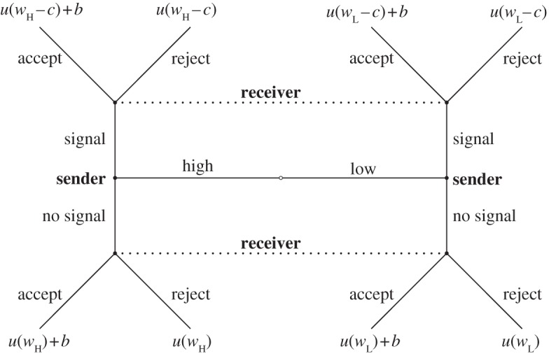
An action–response game with costly signals and partial conflict of interest. The game begins at the central node (open circle). The first move is a move by ‘nature’ to determine the type of the signaller; this type is revealed to the signaller but not the receiver. In the second move, the signaller conditions its behaviour on its type and chooses whether or not to send a signal. As the third move, the receiver must choose between two actions. The receiver can condition on the signal, but not the type; this uncertainty is represented by the dotted lines. Only the pay-offs to the signaller are shown at the terminal nodes. Pay-offs to the receiver are 1 if accepting a high individual or rejecting a low individual, and 0 otherwise.

This baseline model demonstrates that when signallers are risk averse (or equivalently, when the utility of money is concave), it is possible to signal wealth by an ‘ideal handicap’ [18], directly burning some fraction of one's endowment.

3.2. Stochastic signalling

To model stochastic signal cost, we alter the game described above by letting the cost for a particular signal be drawn from some probability distribution rather than being a fixed cost. Thus, instead of burning an amount of money c, a signaller now takes a risk where the amount of money lost, Z, is a random variable. In this case, we can obtain the signaller's expected pay-offs from the utility function. Now a signalling equilibrium will exist when the lottery Z that describes the stochastic signal cost satisfies

and

A lottery z that minimally allows honest signalling in this game thus satisfies

Example 3.1. —

Suppose the signaller has a logarithmic utility function of the form u(x) = log₂(x + 1). Also suppose that the lottery Z that describes the cost in the stochastic game takes value −c₂ with probability p and value 0 with probability 1 − p, where 0 < p < 1 and c₂ > 0. For this example, we will let p = 1/4. Suppose that the low-quality signallers have wealth level w_L = 1, and the high-quality signallers have wealth level w_H = 2. Finally, suppose that the benefit to a signaller of being accepted is b = 1 util.

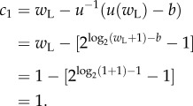
In the deterministic game, the minimal cost c₁ needed to make the low-quality signallers have no incentive to signal is given by u(w_L − c₁) + b = u(w_L) and thus,

This signal cost gives high-quality signallers a pay-off of

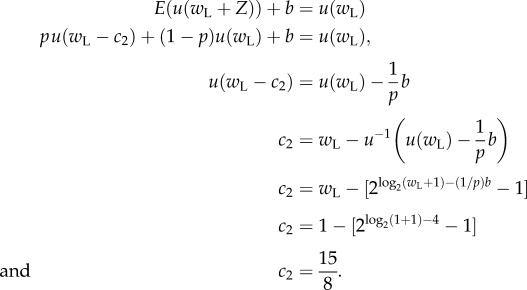
In the stochastic game, the minimal value c₂ needed to ensure that the low-quality signallers have no expected gain from signalling is given by

Thus, the expected loss of wealth is (1/4)(15/8) = 15/32, which is substantially less than the loss of 1 unit of wealth owing to signalling in the deterministic game. This cost gives high-quality signallers an expected pay-off of

which is greater than the pay-off of 2 to a high-quality signaller in the deterministic game. So in this example, stochasticity decreases the average cost of signalling both in wealth and in utility.

We want to understand the differences between the stochastic and deterministic signalling games in general, and discover whether the outcome of the example above is typical. First, we can say that signallers will lose less money on average in the stochastic game than in the deterministic game. This is because signallers will not have to spend as much wealth on average in the stochastic game. Because signallers are risk averse, their expected utility from a fixed wealth is higher than their expected utility from a lottery with the same expected value. Therefore, in order to maintain the same average utility level (the level at which it is worthwhile to signal) in the stochastic game as in the deterministic game, the expected wealth loss must be less. Next, we want to know whether signallers will be better off playing the stochastic game or the deterministic game. This amounts to asking in which game will there be less loss in expected utility owing to the costs of signalling.

3.3. Stochasticity decreases average signal cost

Before stating our results for the discrete case, we describe the basic economic concepts of certainty equivalents and the coefficient of absolute risk aversion. For any utility function u, the certainty equivalent of some lottery X is the certain wealth level that has the same utility as the expected utility of the lottery X. We will write this as C(X). An example is shown in figure 3. Because u is concave, that is the second derivative is negative, the certainty equivalent C(X) is less than E(X), the expected value of X. It turns out that the certainty equivalent depends on the coefficient of absolute risk aversion, which is given by .

Proposition 3.2. —

A successful signaller in the stochastic game will have higher expected utility than a successful signaller in the deterministic game if and only if the players have DARA.

Proof. —

First consider the deterministic game. Let c be the maximum amount of money that a low-quality signaller can spend to obtain the reward without receiving a net loss in utility. Thus, c is defined by the equation

3.1

Therefore, in order to be successful, a high-quality signaller must pay a cost of c + ε₁, for some arbitrarily small ε₁ > 0, and will receive a utility of

Now consider the stochastic game. Let Z be any random variable with a distribution described by some non-degenerate lottery (i.e. Z takes more than one possible value) such that

3.2

So if a low-quality signaller risks money in the lottery Z in order to gain the reward, his expected utility will not increase. Therefore, a high-quality signaller can be successful by risking money in the lottery with outcome Z − ε₂, for some arbitrarily small ε₂ > 0, and will receive an expected utility of

Thus, a successful signaller in the stochastic game will have higher expected utility than a successful signaller in the deterministic game when

As the epsilons are arbitrarily small, we may move them outside the utility functions and cancel them out along with the b on both sides to get

3.3

We now show that this condition holds when the players have DARA. Define utility function u₊ by

Rewriting inequality (3.3) using u₊, we have

As u₊ is increasing, so is and we can write

and

Equation (3.1) allows us to rewrite the right-hand side

and from equation (3.2), this gives us

This last line says that the certainty equivalent of the lottery w_L + Z is greater for utility function u₊ than for u. As the choice of w_L is arbitrary, this is equivalent to the statement that u exhibits greater absolute risk aversion than u₊ (for example, Mas-Colell et al. [19]). As u₊(x) = (x + a) where a = w_H − w_L > 0, this means that u exhibits DARA. So a successful signaller in the stochastic game will have higher expected utility than a successful signaller in the deterministic game precisely when the players have DARA.▪

Figure 3.

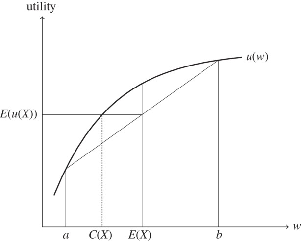
The certainty equivalent C(X) of a lottery X is the certain wealth amount such that its utility is equal to the expected utility of the lottery X. Illustrated here is the certainty equivalent of the lottery X that pays a with probability 1/2 and b with probability 1/2.

The next proposition states what probability distribution on the cost of signalling will maximize the utility and wealth level of successful signallers in the stochastic game. We suppose that the lottery Z that describes this cost has a range that is restricted to some interval [α, β].

Proposition 3.3. —

If the signallers have DARA, the expected utility of a successful signaller is maximized when the distribution for Z assigns positive probability only to the endpoints α and β. This also maximizes the expected wealth level of signallers with concave utility (DARA or otherwise).

Proof. —

As a preliminary note, if h is a convex function and X is some random variable with E(X) fixed that takes values within [α,β], then the distribution for X that maximizes E(h(X)) assigns positive probability only to the endpoints α and β. For suppose that to the contrary there is a distribution for X with some probability mass not at the extreme points. Suppose c is a point between α and β that has some positive probability p > 0. Let ε > 0 be a positive number with magnitude less than the distance between α and c and the distance between c and β. Then consider the distribution where c has zero probability but c − ε and c + ε each have probability increased by p/2. Then E(X) is not changed, but since h is convex, . Thus, E(h(X)) is increased and so our supposition that there exists a distribution for X with some probability mass not at the extreme points that maximizes E(h(X)) is contradicted.

As a high-quality signaller can be successful by risking money in the lottery Z, a low-quality signaller must be just barely unwilling to risk money in this lottery. This gives us the constraint on Z

3.4

for some arbitrarily small ε > 0. In other words, the distribution for Z is constrained by the fact that E(u(w_L + Z)) is constant.

The expected utility of a successful signaller is then

where we define u₊(x) = u(x + w_H − w_L) as in the proof of proposition 3.2.

As u is increasing, so is u₊, and this implies that there exists an increasing function g such that u(x) = g(u₊(x)) for all x. If u exhibits DARA, than u₊ has lower absolute risk aversion than u and this means that g is concave. (See again [19].) Therefore, there exists a convex function h = g^–1 such that u₊(x) = h(u(x)) for all x. This gives us

and so we can find the distribution of u(w_L + Z) that maximizes E(h(u(w_L + Z))). Now E(u(w_L + Z)) is constant, so because h is convex, this distribution is the one that assigns positive probability only to the extreme points, which are u(w_L + α) and u(w_L + β) (see note above). Therefore, the distribution for Z that maximizes the expected utility of a successful signaller is the one that assigns positive probability only to the endpoints α and β.

As u⁻¹ is also convex regardless of whether u exhibits DARA, as long as u is concave, an analogous argument shows that the expected wealth level of a successful signaller is also maximized when the distribution for Z assigns positive probability only to the endpoints α and β.▪

4. Continuous signalling

In our discrete model, there are only two types of signaller, two options for signalling and two types of response. Alternatively, we imagine a situation where there are signallers with many different wealth levels, many possible signal intensities and receivers may choose many different responses. The extreme case is when wealth levels, signal intensities and responses may come from any point along a continuum. This produces a continuous signalling game—a class of model which has been instrumental in the development of the theory of costly signalling (for example, Grafen [20]). In Grafen's biological interpretation, each signaller has a ‘quality’ instead of a wealth level. Receivers are typically thought of as potential mates. Receivers must gauge a signaller's quality based on the signal intensity, and do best to respond more enthusiastically the higher the signaller's quality.

Following the notation of Bergstrom et al. [21], signallers have a pay-off function π(q,s,r) that depends on their own quality (q), the intensity of the signal they send (s) and the level of response they receive from the receiver (r). This pay-off function is conceived of as the difference of a benefit function H(q,r) and a cost function C(q,s). The benefit depends on the quality of the signaller and the response it receives, and the cost depends on the quality of the signaller and the intensity of the signal that it chooses to send. Each receiver has a pay-off function G(q,r) that depends on how appropriate the response (r) is given the signaller's true quality (q). Of course, the receiver knows only what signal intensity (s) the signaller chose. A strategy for signallers is a function s = s(q) that specifies a choice of signal intensity for all signaller qualities q. A strategy for a receiver is a function r = r(s) that specifies a choice of response for all signal intensities that the signaller might send. If the functions s(q) and r(s) make up a signalling equilibrium, this means that the function s is one-to-one and that neither player can benefit by unilaterally modifying its strategy function.

Bergstrom et al. [21] give a method of finding the functions s(q) and r(s) that make up a signalling equilibrium for any particular game of the above form. Building upon this method, we prove that when signallers have DARA, stochasticity decreases average signal cost in continuous signalling games as well as in discrete games.

As we did for the discrete case, we will describe two signalling games, one deterministic and one stochastic, and compare the average pay-offs at equilibrium. For both games, we assume that benefit is proportional to response level and that signal intensity is proportional to signal cost. The receiver's pay-off G(q,r), for how appropriate the response is given the signaller's true quality, is also the same for both games. We will call the signal intensity functions for the deterministic and stochastic games S_B and S_G, respectively (for Burning money or Gambling money). So for the deterministic game, a signal of intensity S_B will cost S_B units of wealth. For the stochastic game, a signal of intensity S_G will cost S_G units of wealth with probability p and 0 units of wealth with probability 1 − p, where 0 < p < 1.

For the deterministic regime, the pay-off to a successful signaller with wealth level w_H in the discrete game was

where c is the signal cost and b is the benefit of being accepted by the receiver. In the continuous case, cost is proportional to signal intensity and the benefit is proportional to response level. This gives us

4.1

as the pay-off function for signallers in the continuous game with deterministic costs.

In the stochastic regime, the pay-off to a successful signaller with wealth level w_H in the discrete game was b + u(w_H + Z) giving an expected pay-off of

Exchanging r for b and q for w_H gives us the expected pay-off for a signaller in the continuous case

The lottery Z takes value −S_G with probability p and value 0 with probability 1 − p. Therefore, we can write

4.2

Having defined the strategy space and pay-off functions for both games, the problem now is to find a general solution for the equilibrium response functions of the signal intensities and signal intensity functions of quality. We give the proof of the following proposition in Appendix A.

Proposition 4.1. —

If the players have DARA, then at equilibrium they will have higher expected utility in the stochastic signalling game than in the deterministic signalling game.

5. Discussion

Signalling models in both biology and economics have typically assumed determinate costs. In the real world, signal costs will often if not always be stochastic. This difference matters. Here, we show that when signallers have realistic risk preferences, stochastic signal costs result in signals that are cheaper, on average, than when signals have determinate costs. This comparative result holds in discrete and continuous models alike.

In biology, signal costs may be stochastic for a variety of reasons. Begging calls are probably costly because of stochastic predation risk instead of determinate energy expenditures [22–25]. Physical ornamentation such as long tails or colourful plumage in birds may similarly be costly owing to predation risk [26]. Extravagant territorial and courtship displays can be risky as well: instead of storing resources for lean times, an individual invests time and energy in prolonged displays [27].

Many if not most biological instances of stochastic signal costs will be more complicated in form than the simple lotteries modelled here. The important point is that our analysis shows that to simply treat stochastic costs as equivalent to their expectation will often lead to a distorted picture of the true costs. And our results suggest that variable signal costs, rather than undermining honesty in costly signalling, in fact bolster it.

Empirical studies could provide evidence for the action of gambles to decrease average signal costs. The greater the variance in the stochastic cost of a signal, the more likely it is that the signal cost is being reduced by the stochasticity (see proposition 3.3). This suggests the need for empirical studies to take into account risk structure when measuring signal costs. If the risk structure has high variance, then high average cost is not as important for honest signalling.

In the last couple decades, researchers have described a number of systems in which honest communication is less costly than in traditional handicap theory. Such efforts are essential if we are to explain the large number of different contexts in which communication is found to be stable. The effects of stochasticity for decreasing signal costs is another fundamental mechanism that deserves attention because of the wide variety of circumstances in which it likely acts.

Funding statement

This work was supported by NSF grant no. EF-1038590 to C.T.B.

Appendix A. Proof of proposition 4.1

We first use the method from Bergstrom et al. [21] to obtain differential equations for the signalling strategy under burning money, S_B(q), and under gambling money, S_G(q). For burning money, the signaller's pay-off function is

We can break this function into the difference of a benefit function H(q,r) that depends on the signaller's quality q and the receiver's response level r, and a cost function C_B(q,S_B) that depends on q and the signal intensity, S_B. Indeed, if

A1

then π_B = H − C_B.

Similarly, for gambling money, we have

which is broken down into π_G = H − C_G as follows:

A2

Following Bergstrom et al. [21], we obtain the differential equation

which provides the slope of the signalling strategy S(q) in terms of the benefit function H, the cost function C (which depends on S(q) itself) and the equilibrium response level R*(q).

From expressions (A 1) and (A 2), we see that ∂H/∂r = 1. And if we denote by r′(q) the derivative dR*/dq, then for burning money,

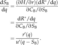A3

And for gambling money,

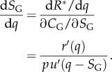A4

As the benefit function H is the same for both games, and at the separating equilibrium the receiver's response r will be the same for both games, signallers in the stochastic game will do better than signallers in the deterministic game when C_G < C_B. Therefore, we want to show that when u exhibits DARA, C_G < C_B. To do so, we first show that C_G < C_B is equivalent to inequality (A 7) below, and then show that inequality (A 7) follows when u exhibits DARA.

From equations (A 1) and (A 2), C_G < C_B gives us

i.e.

A5

Rewriting to isolate S_G, we have

As u is increasing, so is u⁻¹. Thus, C_G < C_B when

Define

A6

so that C_G < C_B if .

Note that is a function of q and consider the value of the differential equation (A 4), i.e.

along the curve . Note that if for q > 0 then for q > 0 because . So C_G < C_B when , that is when . Substituting for

Simplifying the left-hand side and evaluating the derivative on the right-hand side,

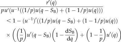Applying the inverse rule for derivatives, we get

Multiplying by the (positive) denominator of the left-hand side yields

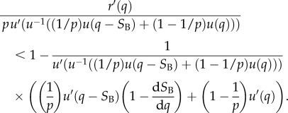
Rearranging and substituting expression (A 3) gives

And after a bit of algebra, we obtain

If we let d = u(q) − u(q − S_B) be the distance between u(q) and u(q − S_B), the above inequality becomes

A7

This inequality has a nice geometric interpretation, illustrated in figure 4. It says that the derivative of u at point M is less than the weighted average of the derivative at points L and N.

Figure 4.

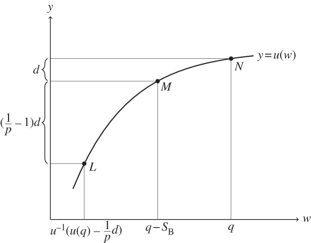
Inequality (A 7) says that the derivative of u at point M is less than the weighted average of the derivatives at L and N. Note that the weighted average of y = u(q) and .

We now show that inequality (A 7) follows when u exhibits DARA. We first point out that the statement that u exhibits DARA is equivalent to the statement that the rate of decrease of u′(w), with respect to y, is decreasing. Thus, in figure 4, u′ decreases proportionately more from L to M than from M to N. Thus, u′ at N is not small enough to balance out the value of u′ at L, and so the weighted average is greater than the single value u′(q − S_B).

Indeed, if u exhibits DARA, then by definition −u″(w)/u′(w) is decreasing in w. As u⁻¹ is increasing, this implies that −u″(u⁻¹(y))/u′(u⁻¹(y)) is decreasing in y. Thus,

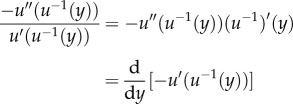is decreasing as well (the above equalities follow from the inverse rule of derivatives and the chain rule, respectively). So the rate of decrease of u′(w), with respect to y, is decreasing.

This means that, in figure 4, the difference between u′ at L and u′ at M is more than (1/p − 1) times the difference between u′ at M and u′ at N. Let's call these differences D₁ and D_2, respectively, so we have D₁ >(1/p − 1)D₂. Therefore, by the definitions of D₁ and D₂,

Rearranging, we get

which is inequality (A 7). So DARA gives us inequality (A 7), which is equivalent to C_G < C_B, and we have proved the result.

A.1. Equilibrium stability

We next apply the second part of Bergstrom et al.'s result to show that the equilibrium strategies S_B(q) and S_G(q) we found above are stable (i.e. the extrema are maxima rather than minima). Their result states that the equilibrium is stable when the following second-order condition holds everywhere along the solution curve.

A8

We have H(q,r) = r + u(q). So

Thus,

and so

Also,

For the cost function, we have C(q,s) = u(q) − u(q − s) for burning money and C(q,s) = p(u(q) − u(q − s)) for gambling money. For burning money, this gives us

and

For gambling money, we have

For both cases, inequality (A 8) then reduces to

where δ is either 1 or p. As u is increasing, u′ is positive, so the above inequality holds when u″(q − s) is negative, that is when utility is concave. Thus, the second-order condition holds because we are only considering individuals with concave utility.

References

- 1.Maynard Smith J, Harper D. 2003. Animal signaling. Oxford, UK: Oxford University Press. [Google Scholar]
- 2.Bradbury JW, Vehrencamp SL. 2011. Principles of animal communication, second edition. Sunderland, MA: Sinauer Associates. [Google Scholar]
- 3.Riley JG. 2001. Silver signals: twenty-five years of screening and signaling. J. Econ. Lit. 39, 432–478. ( 10.1257/jel.39.2.432) [DOI] [Google Scholar]
- 4.Számadó Sz. 2011. The cost of honesty and the fallacy of the handicap principle. Anim. Behav. 81, 3–10. ( 10.1016/j.anbehav.2010.08.022) [DOI] [Google Scholar]
- 5.Bergstrom CT, Lachmann M. 1997. Signalling among relatives. I. Is costly signalling too costly? Phil. Trans. R. Soc. Lond. B 352, 609–617. ( 10.1098/rstb.1997.0041) [DOI] [Google Scholar]
- 6.Hurd PL. 1995. Communication in discrete action–response games. J. Theor. Biol. 174, 217–222. ( 10.1006/jtbi.1995.0093) [DOI] [Google Scholar]
- 7.Getty T. 1998. Reliable signalling need not be a handicap. Anim. Behav. 56, 253–255. ( 10.1006/anbe.1998.0748) [DOI] [PubMed] [Google Scholar]
- 8.Számadó Sz. 1999. The validity of the handicap principle in discrete action–response games. J. Theor. Biol. 198, 593–602. ( 10.1006/jtbi.1999.0935) [DOI] [PubMed] [Google Scholar]
- 9.Lachmann M, Számadó Sz, Bergstrom CT. 2001. Cost and conflict in animal signals and human language. Proc. Natl Acad. Sci. USA 98, 13 189–13 194. ( 10.1073/pnas.231216498) [DOI] [PMC free article] [PubMed] [Google Scholar]
- 10.Robson AJ. 1990. Efficiency in evolutionary games: Darwin, Nash, and the secret handshake. J. Theor. Biol. 144, 379–396. ( 10.1016/S0022-5193(05)80082-7) [DOI] [PubMed] [Google Scholar]
- 11.Maynard Smith J. 1994. Must reliable signals always be costly? Anim. Behav. 47, 1115–1120. ( 10.1006/anbe.1994.1149) [DOI] [Google Scholar]
- 12.Krakauer DC, Pagel M. 1995. Spatial structure and the evolution of honest cost-free signalling. Proc. R. Soc. Lond. B 260, 365–372. ( 10.1098/rspb.1995.0106) [DOI] [Google Scholar]
- 13.Viljugrein H. 1997. The cost of dishonesty. Proc. R. Soc. Lond. B 264, 815–821. ( 10.1098/rspb.1997.0114) [DOI] [Google Scholar]
- 14.Bergstrom CT, Lachmann M. 1998. Signalling among relatives. III. Talk is cheap. Proc. Natl Acad. Sci. USA 95, 5100–5105. ( 10.1073/pnas.95.9.5100) [DOI] [PMC free article] [PubMed] [Google Scholar]
- 15.Silk JB, Kaldor E, Boyd R. 2000. Cheap talk when interests conflict. Anim. Behav. 59, 423–432. ( 10.1006/anbe.1999.1312) [DOI] [PubMed] [Google Scholar]
- 16.Zollman KJS, Bergstrom CT, Huttegger SM. 2013. Between cheap and costly signals: the evolution of partially honest communication. Proc. R. Soc. B 280, 20121878 ( 10.1098/rspb.2012.1878) [DOI] [PMC free article] [PubMed] [Google Scholar]
- 17.Chiappori PA, Paiella M. 2011. Relative risk aversion is constant. Econ. Rev. 93, 1021–1052. ( 10.1111/j.1542-4774.2011.01046.x) [DOI] [Google Scholar]
- 18.Hasson O. 1997. Towards a general theory of biological signaling. J. Theor. Biol. 185, 139–156. ( 10.1006/jtbi.1996.0258) [DOI] [PubMed] [Google Scholar]
- 19.Mas-Colell A, Whinston MD, Green JR, et al. 1995. Microeconomic theory. New York, NY: Oxford University Press. [Google Scholar]
- 20.Grafen A. 1990. Biological signals as handicaps. J. Theor. Biol. 144, 517–546. ( 10.1016/S0022-5193(05)80088-8) [DOI] [PubMed] [Google Scholar]
- 21.Bergstrom CT, Számadó S, Lachmann M. 2002. Separating equilibria in continuous signalling games. Phil. Trans. R. Soc. Lond. B 357, 1595–1606. ( 10.1098/rstb.2002.1068) [DOI] [PMC free article] [PubMed] [Google Scholar]
- 22.McCarty JP. 1996. The energetic cost of begging in nestling passerines. Auk 113, 178–275. ( 10.2307/4088944) [DOI] [Google Scholar]
- 23.Leech SM, Leonard ML. 1997. Begging and the risk of predation in nestling birds. Behav. Ecol. 8, 644–646. ( 10.1093/beheco/8.6.644) [DOI] [Google Scholar]
- 24.Briskie JV, Martin PR, Martin TE. 1999. Nest predation and the evolution of nestling begging calls. Proc. R. Soc. Lond. B 266, 2153–2159. ( 10.1098/rspb.1999.0902) [DOI] [Google Scholar]
- 25.Haskell DG. 1999. The effect of predation on begging-call evolution in nestling wood warblers. Anim. Behav. 57, 893–901. ( 10.1006/anbe.1998.1053) [DOI] [PubMed] [Google Scholar]
- 26.Moller AP, Nielsen JT. 1997. Differential predation cost of a secondary sexual character: sparrowhawk predation on barn swallows. Anim. Behav. 54, 1545–1551. ( 10.1006/anbe.1997.9998) [DOI] [PubMed] [Google Scholar]
- 27.Zahavi A, Zahavi A. 1997. The handicap principle. Oxford, UK: Oxford University Press. [Google Scholar]