Simplifying biochemical models with intermediate species

Abstract

Mathematical models are increasingly being used to understand complex biochemical systems, to analyse experimental data and make predictions about unobserved quantities. However, we rarely know how robust our conclusions are with respect to the choice and uncertainties of the model. Using algebraic techniques, we study systematically the effects of intermediate, or transient, species in biochemical systems and provide a simple, yet rigorous mathematical classification of all models obtained from a core model by including intermediates. Main examples include enzymatic and post-translational modification systems, where intermediates often are considered insignificant and neglected in a model, or they are not included because we are unaware of their existence. All possible models obtained from the core model are classified into a finite number of classes. Each class is defined by a mathematically simple canonical model that characterizes crucial dynamical properties, such as mono- and multistationarity and stability of steady states, of all models in the class. We show that if the core model does not have conservation laws, then the introduction of intermediates does not change the steady-state concentrations of the species in the core model, after suitable matching of parameters. Importantly, our results provide guidelines to the modeller in choosing between models and in distinguishing their properties. Further, our work provides a formal way of comparing models that share a common skeleton.

1. Introduction

Systems biology aims to understand complex systems and to build mathematical models that are useful for inference and prediction. However, model building is rarely straightforward, and we typically seek a compromise between the simple and the accurate, shaped by our current knowledge of the system. Two models of the same system, potentially differing in the number of species and the form of reactions, might have different qualitative properties and the conclusions we draw from analysing the models might be strongly model-dependent. The predictive value and biological validity of the conclusions might thus be questioned. It is therefore important to understand the role and consequences of model choice and model uncertainty in modelling biochemical systems.

Transient, or intermediate, species in biochemical reaction pathways are often ignored in models or grouped into a single or few components, either for reasons of simplicity or conceptual clarification, or because of lack of knowledge. For example, models of the multiple phosphorylation systems vary considerably in the details of intermediates [1,2], and intermediates are often ignored in models of phosphorelays and two-component systems [3,4]. Typically, intermediate species are protein complexes such as a kinase–substrate protein complex. It has been shown that sequestration of intermediates can cause ultrasensitive behaviour in some systems [5,6]. Therefore, the inclusion/exclusion of intermediates is a matter of considerable concern.

As an example, consider the transfer of a modifier molecule, such as a phosphate group in a two-component system, from one molecule to another: , where A, B are unmodified forms (without the modifier group), A*, B* are modified forms (with the modifier), indicate reversible reactions, and … are potential transient reaction steps. Two-component systems are ubiquitous in nature and vary considerably in architecture and mechanistic details across species and functionality [7]. Whether or not the specifics are known beforehand, it is customary to use a reduced scheme such as [3,4].

We use chemical reaction network theory (CRNT) to model a system of biochemical reactions and assume that the reaction rates follow mass-action kinetics. The polynomial form of the reaction rates has made it possible to apply algebraic techniques to learn about qualitative properties of models, without resorting to numerical approaches [8–14]. Building on previous works [15–17], we propose a mathematical framework to compare different models and to study the dynamical properties of models that differ in how intermediates are included. The most fundamental and crucial dynamical features are the number and stability of steady states. We assume that the kinetic parameters are unknown and study the capacity of each model to exhibit different steady-state features.

The paper is organized in the following way. We first introduce the concepts of a core model and an extension model. An extension model is constructed from the core model by including intermediates. Next, we discuss how the steady-state equations of different models are related and illustrate the findings with an example. We proceed to discuss the number of steady states of core and extension models. After that, we introduce the steady state classes, a key concept of this paper. Extension models in the same steady-state classes have the same properties at steady state (provided the parameter sets of the two models can be matched, in some sense). Using these ideas, we build a decision tree to guide the modeller in choosing a model and in understanding the consequences of choosing a particular model. Finally, we illustrate our approach with an example based on two-component systems. All proofs and mathematical details are in the electronic supplementary material.

2. The core model and its extensions

We use the notation and formalism of CRNT [18,19]. A reaction network is defined as a set of species, denoted by capital letters (e.g. A, B, C), a set of complexes and a set of reactions between complexes. Each complex is a combination of species, for example y₁ = A + B or y₂ = 2C (not to be confused with a protein complex). A potential reaction could be A + B → 2C, or also written simply y₁ → y₂. A reaction is not necessarily reversible, that is, we can have A + B → 2C without having the reverse reaction 2C → A + B. Whenever a reaction is reversible, we model it as two separate irreversible reactions. We assume that each reaction occurs according to mass-action kinetics, that is, at a rate proportional to the product of the species concentrations in the reactant or source complex [20]. For example, the reaction A + B → 2C occurs at a rate k[A][B], where [A], [B] are the concentrations of the species A, B and k is a reaction-specific positive constant. Reaction networks are often drawn graphically as shown in figure 1a–e. Figure 1c–e is schematic of reaction networks: only the structure of the network is shown, and neither the species nor the rate constants are indicated.

Figure 1.

Representation of reaction networks: (a,b) detailed representation; (c–e) schematic representation. (a) and (e) are core models and (b–d) are extended models of (a) and (e). (a) A reaction network with complexes S₀ + E, S₁ + E, S₂ + E (enclosed in dashed boxes). Each reaction is labelled with its rate constant (k or ). (b) An extension model of network (a) with intermediate Y. (c) The complex y₁ is involved in a reversible ‘dead-end’ reaction with one intermediate. (d) The complex y₁ is converted into Y, which splits into y₂ or y₃, respectively (the former reversibly). (e) Schematic of (a).

Figure 1a corresponds to a simple enzymatic mechanism where E is an enzyme and S_j is a substrate with j = 0,1,2 phosphorylated sites. The substrate S₀ can be doubly phosphorylated sequentially via S₁ or directly (processively). In figure 1b, a transient product Y formed by S₀ and E, or by S₁ and E (these are often denoted by S₀ · E and S₁ · E) is shown. In the particular case, we do not distinguish between the two transient products (which might be unrealistic, but it serves an illustrative purpose).

An intermediate is defined as a species in a reaction network that is created and dissociated in isolation, that is, it is produced in at least one reaction, consumed in at least one reaction and it cannot be part of any other complex (e.g. Y in figure 1b–d). A core model is the minimal reaction mechanism to be modelled. Each reaction y_i → y_j in the core model consists of two core complexes y_i, y_j. The species contributing to the core complexes are referred to as core species. An extension model is any reaction network such that

• (i) the set of complexes consists of core complexes and some intermediates that are not part of the core model;

• (ii) reactions are between two core complexes, two intermediates or between an intermediate and a core complex; and

• (iii) the core model is obtained from the extension model by collapsing all reaction paths y_i → Y₁ → … → Y_k → y_j, where Y_i are intermediates, into a single reaction y_i → y_j.

Some examples are given in figure 1. Figure 1b is an extension model of figure 1a and figure 1c and d are extension models of figure 1e. Figure 1a is a concretization of figure 1e. Note that the directionality of the reaction arrows needs to be preserved. For instance, in figure 1e, an extension of the reaction y₁ → y₂ cannot be , because it would imply that y₂ → y₁ also is in the core model. By adding arbitrarily many intermediates (e.g. ), we can create arbitrarily many extension models with the same core.

Under mass-action kinetics, the dynamics of figure 1b is described by a polynomial system of ordinary differential equations (ODEs):

2.1

where k_* are rate constants, [X] denotes the concentration of species X and is the instantaneous change in [X]. In addition, there are two conservation laws,

2.2

that is, quantities that are conserved over time and determined by the initial concentrations. Conservation laws confine the dynamics to an invariant space given by and (referred to as conserved amounts), and the dynamical analysis must be restricted to this space. The invariant spaces are called stoichiometric classes in the CRNT literature. If we consider a maximal set of independent conservation laws, then the species that appear in the conservation laws are independent of the chosen set.

The core model in figure 1a has two conservation laws,

2.3

The two sets of conservation laws, (2.2) and (2.3), differ by a linear combination of intermediate concentrations (here a single term). This similarity between (2.2) and (2.3) holds generally.

Theorem 2.1. —

The conservation laws in the core model are in one-to-one correspondence with the conservation laws in any extension model. The correspondence is obtained by adding a suitable linear combination of the [Y]'s to each conservation law of the core model.

Theorem 2.1 does not depend on the assumption of mass-action kinetics but relies on the structure of the network only, that is, on the set of reactions of the network.

3. Steady-state equations

We next state theorems 3.1 and 3.2 that allow us to relate the dynamics near steady states of the core and extension models to each other.

At steady state for all species X. Under the assumption of mass-action kinetics, this condition translates into a system of polynomial equations in the species concentrations. A way to solve the equations is to express one variable in terms of other variables. This expression must then be satisfied by any solution to the system. We let [y] denote the product of the species concentrations in complex y, for example, [2S] = [S]² and [S₀ + E] = [S₀][E]. Different extension models contain different intermediates, resulting in different steady-state equations. Because the intermediates always appear as linear terms in the steady-state equations of an extension model (see (2.1)), they can be eliminated from the equations and written in terms of the concentrations of the core species.

Theorem 3.1. —

Using the equations for all intermediates in the extension model, the steady-state concentrations of the intermediates Y are given as linear sums of products of the core species concentration [17,21]. The constant μ_Y,y is either zero or positive and depends only on the rate constants of the extension model. [y] appears in the expression, that is, μ_Y,y ≠ 0, if and only if there is a reaction path y→ … →Y involving exclusively intermediates.

As a consequence of the theorem, once the steady-state concentrations of the core species are known, the steady-state concentrations of the intermediates are also known. Because μ_Y,y ≥ 0 and at least one of the constants is non-zero (all intermediates are produced), positive steady-state concentrations of the core species lead to positive concentrations of the intermediates.

Theorem 3.1 makes explicit use of mass-action kinetics. It remains true for non-mass action kinetics in the sense that an explicit expression for [Y] can be found if all reactions have mass-action reaction rates, whereas all other reactions can have arbitrary reaction rates. In that case, however, the form of the expression might not be polynomial nor lead to positive concentrations.

The manipulations leading to the expression from are purely algebraic and do not require any assumptions about the conserved amounts. In example (2.1), the equation gives

3.1

where are reciprocal Michaelis–Menten constants [20]. If (3.1) is substituted into (2.1), we obtain a new ODE system:

3.2

which is a mass-action system for the core model in figure 1a with , and (as ). We say that the rate constants are realized by and that k_* and are a pair of matching rate constants. In the particular case, are realized by choosing , and any , such that . Choosing k₂ fixes the values of m₁, m₃ in  (3.1). However, for some (unrealistic) extension models, not all choices of rate constants of the core model are realizable (see electronic supplementary material).

The relation between the ODEs in figure 1a,b holds generally for any pair of core and extension models.

Theorem 3.2. —

After substituting the expressions into the ODEs of the extension model, we obtain a mass-action system for the core model.

The quasi-steady-state approximation (QSSA) proceeds similarly [22]. An equation of the form is used to find an expression for [Y] in terms of [y] under the additional assumptions that certain species are in high or low concentration. This expression is subsequently substituted into the remaining ODEs to reduce the system. Theorems 3.1 and 3.2 show that this always can be performed, irrespective of any biological justification of the procedure.

As a consequence of the theorems, the steady states of an extension model can be found in this way: we first solve the equations for [Y] in terms of [y] (theorem 3.1) and then insert the expressions for [Y] into the remaining steady-state equations (theorem 3.2). The steady states of the extended model are now found by solving the steady-state equations for the core model to obtain the concentrations of the core species. This corresponds to solving (3.2) in the abovementioned example. The obtained values are subsequently plugged into the expressions given in theorem 3.1 to find the steady-state values of the intermediates. That is, for matching rate constants between the core and an extension model, the solutions to the steady-state equations of the core model completely determine the solutions to the steady-state equations of the extension model.

The conservation laws, however, impose different constraints on the steady-state solutions for given conserved amounts. Specifically, by inserting (3.1) into (2.2), we obtain

3.3

The steady states of the extension model solve (3.2) and (3.3), whereas they solve (3.2) and  (2.3) in the core model. Equation (3.3) is nonlinear in the concentrations of the core species. Nonlinear terms in the conservation laws can cause the two models to have substantially different properties. This is reflected in the example in §4.

Importantly, if the system has no conservation law, then addition of intermediates cannot alter any property of the core model at steady state. This will be the case, for instance, when production and degradation of all core species in the model are explicitly modelled.

4. An example

The number of steady-state solutions for the core model and an extension model can differ substantially. For matching rate constants, the steady states of each system are found by intersecting the steady-state equations for the core species with the conservation laws of each of the systems. The number of points in this intersection might differ between extension models and the core model, depending on the form of the conservation laws.

We illustrate this using the two-site phosphorylation system in figure 1a and include dephosphorylation reactions

4.1

In addition, we add the reactions

4.2

The motivation for the addition is not biological but for illustrative reasons. It allows us to plot the steady-state equations in two dimensions. We will consider the positive steady states of the core model in figure 1a together with (4.1) and (4.2), and the extension model in figure 1c together with (4.1) and (4.2), and y₁ = S₀ + E, y₂ = S₁ + E, y₃ = S₂ + E. The added reactions are core reactions and do not involve intermediates. Because the substrate S₂ is degraded (S₂ → 0), the total amount of substrate is no longer conserved and there is only one conservation law, namely that for the kinase (compare (2.3)).

At steady state, the core and any extension model fulfil the relation

4.3

for some constants a₁, a₂ > 0 that depend on the rate constants of each model (see electronic supplementary material).

The relation is obtained from the steady-state equations of the core model alone and therefore must be fulfilled by all extension models for matching rate constants (theorem 3.2). One can show that the concentrations of [S₁] and [S₂] at steady state are uniquely determined by [E] and [S₀] (see electronic supplementary material).

For a given conserved amount for the kinase, the steady-state concentrations are determined by the common points of the graph of (4.3) and the curve for the conservation law. For the core model, this curve is , which is a vertical line in the ([E], [S₀])-plane. Because (4.3) is strictly decreasing in [E], it follows that there is a single steady state for any choice of (figure 2a).

Figure 2.

The steady-state curve (4.3) for a₁ = 2, a₂ = 0.5 (dashed) together with the curve for the conservation law. The steady states for a fixed conserved amount are the intersection points of the two curves (dashed and solid lines). (a) Core model. Conservation law curves (solid) for different values of . (b) Extension model. Conservation law curves (solid) as in (4.4) for different values of and a₃ = 2. (c) Extension model. Conservation law curves (solid) as in (4.4) for different values of a₃ and . (Online version in colour.)

Consider next the extension model corresponding to figure 1c (with the modifications introduced in (4.1) and (4.2)). For arbitrary fixed rate constants of the core model, we choose rate constants of the extension model that realize the rate constants of the core model. This can always be achieved for extension models with ‘dead-end’ complexes, like that of figure 1c (see electronic supplementary material). For , the concentration of the intermediate is [Y] = a₃[E][S₀] for some constant a₃ > 0 that depends on the rate constants of the extension model. Consequently,

4.4

If a₃ = 0, then we obtain the core model. In the particular case, a₃ varies independently of a₁, a₂ and all values of a₃ can be obtained when realizing the rate constants of the core model. Combining (4.3) and (4.4) yields a second-order polynomial in [E]:

4.5

Hence, for fixed a₁, a₂, a₃, the polynomial can have zero, one or two positive solutions, depending on the value of E_cons^C. Figure 2 shows graphically the steady-state solutions for the core (figure 2a) and the extension (figure 2b,c) model as the intersection of the steady-state equation (4.3) and the curve for the conservation law for different values of and a₃. In figure 2, the curve for the steady-state equation (dashed) is given for a₁ = 2 and a₂ = 0.5 and is the same for the two models. For the core model, the conservation law curve is a vertical line (solid, figure 2a), which intersects the steady-state curve in precisely one point (figure 2a). For the extended model, the conservation law curve (solid, figure 2b,c) is the ratio in (4.4). Depending on the value of , the two curves intersect in zero, one or two points illustrating how the number of steady states vary with (figure 2b, with a₃ = 2). The same conclusion is obtained by varying a₃ while keeping fixed (figure 2c, with ).

In this particular case, we could find explicit expressions for the steady-state concentrations in terms of the conserved amounts and the rate constants. This is not always the case.

5. Number of steady states

In the example in §4, one can choose rate constants and conserved amounts such that the extension model does not have a positive steady state, even though the core model has a positive steady state for all choices of rate constants. However, it is easy to see that a₃ can always be chosen so small that there is at least one positive solution for fixed a₁, a₂ and . If a₃ ≈ 0, then the contribution of [E][S₀] in (4.4) becomes insignificant, and the extension model is ‘similar’ to the core model. This is observed in figure 2c for small a₃, the curve for the conservation law is almost a vertical line.

Therefore, in the example, it is always possible to choose matching rate constants such that the number of steady states in the extension model is at least as big as the number of steady states in the core model, for corresponding conserved amounts. This observation holds generally. We now state the main result concerning the dynamical properties of extension models and the number of steady states.

Theorem 5.1. —

If the core model has N non-degenerate¹ positive steady states for some rate constants and conserved amounts, then any extension model that realizes the rate constants has at least N corresponding non-degenerate positive steady states for some rate constants and conserved amounts. Oppositely, if the extension model has at most one positive steady state for any rate constants and conserved amounts then the core model has at most one positive steady state for any matching rate constants and conserved amounts. The rate constants and conserved amounts can be chosen such that the correspondence preserves unstable steady states with at least one eigenvalue with non-zero real part and asymptotical stability for hyperbolic steady states.

The proof essentially relies on the observation in the previous example that a certain parameter (a₃ in the example) can be chosen so small that the extension model and the core model are almost identical at steady state. The relationship between a reaction network and a subnetwork has been studied previously, but in different contexts. For example in [23,24], where subnetworks are defined by (certain) subsets of reactions, or in [24], where subnetworks are defined by removing species from reactions. Characterizations similar to theorem 5.1 about the number of steady states hold in these situations.

In figure 2, the steady state in the extension model closest to the steady state in the core model (for the same conserved amount) inherits the stability properties of the steady state of the core model. In this case, it is asymptotically stable. However, we cannot conclude anything about the other steady state in the extension model from the core model alone.

6. Steady-state classes and canonical models

The observations made about the conservation laws and the steady-state equations (theorems 2.1, 3.1 and 3.2) suggest that it suffices to know what core complexes contribute to the conservation laws in order to compare the extension and core models at steady state. In figure 1b, the core complexes S₀ + E, S₁ + E contribute to the conservation laws for the kinase and substrate. Any other extension model, contributing the same core complexes to the conservation law, will result in equations for the steady states of the same form. Specifically, if two extension models contribute the same core complexes to the conservation laws and realize the same rate constants,² then the two models are identical at steady state. In particular, we can apply theorem 5.1 to any of the two models.

Therefore, we can group extension models according to the core complexes that appear in the conservation laws. We say that two extension models belong to the same steady-state class if they share the same core complexes in the conservation laws. The complexes characterizing a steady-state class are called the class complexes. We can use theorem 3.1 to provide a graphical characterization of the classes: the core complexes that contain a species appearing in some conservation law are selected. If there exists a reaction from such a core complex to an intermediate, then the core complex is a class complex. The class of the core model is the class with no class complexes.

In figure 3, the graphical characterization is illustrated using the core model in figure 1a, written in simplified form. All species appear in some conservation law, and hence all core complexes can be class complexes. Consider the extension models in figure 1b and figure 1c,d with y₁ = S₀ + E, y₂ = S₁ + E, y₃ = S₂ + E. The extension model in figure 1c belongs to the steady-state class with class complex y₁, because there is only one path from a core complex to an intermediate: y₁ → Y. Similarly, the extension models in figure 1b,d have class complexes y₁, y₂. We conclude that figure 1b,d are in the same class, whereas the models in figure 1a,c are in different classes and have different equations. In this case, figure 1a has always one steady state for any choice of conserved amounts and rate constants, whereas figure 1b–d can be multistationary (this is proved by direct computation of the steady states in the electronic supplementary material).

Figure 3.

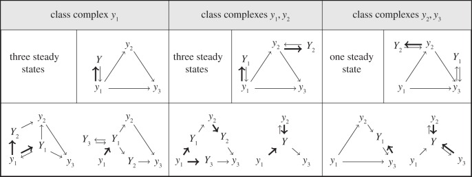
We consider the core model of figure 1a (with y₁ = S₀ + E, y₂ = S₁ + E, y₃ = S₂ + E) and its steady-state classes. Each class is characterized by an extension model (the canonical model) with a dead-end reaction added for each class complex (upper right corner). Each class (except the class of the core model) has an infinite number of members and a few of these are shown. Class complexes are source complexes of a reaction with an intermediate as product (marked in bold in the figure). For the number of steady states we consider the model given in figure 1a and dephosphorylation reactions S₂ → S₁ and S₁ → S₀ (not shown in the figure). The number of steady states in each class refers to the maximal number of steady states that a model in the class can have for some choice of rate constants and total amounts. This has been found by direct computation of the steady states (see electronic supplementary material). Alternatively, the CRN Toolbox could have been used [25].

Because class complexes characterize the steady-state classes, there is a finite number of classes, at most 2^K, with K the number of core complexes (K = 3 in figure 3). The classes are naturally ordered by set inclusion: a class is smaller than another class if the latter contains the class complexes of the former. In particular, the steady-state class of the core model is smaller than any other class. Thus, the class of figure 1a is smaller than the classes of figure 1b–d, then classes of figure 1b,d are the same and the class of figure 1c is smaller than the class of figure 1b. The classes of the models in the first and the third box of figure 3 are not comparable as the first is {y₁} and the last is {y₂, y₃}.

All extension models in a steady-state class have common properties at steady state (subject to the requirement of realizability of rate constants). Thus, it is natural to select a representative for each class with a small number of intermediates and such that the behaviours of all models in the class are reflected in the behaviour of the representative. To each class, we construct a canonical model by adding a dead-end reaction, , for each class complex (see figure 3 for an example). Importantly, the steady-state equations for the canonical model are simpler than for any other extension model in the same class. It is shown in the electronic supplementary material that the parameter space of the canonical model is as large as possible. This leads to the following corollary to theorem 5.1.

Corollary 6.1. —

If the canonical model of a steady-state class has a maximum of N steady states for any rate constants and conserved amounts, then all extension models in the class, or in any smaller class, have at most N steady states.

In particular, if the largest canonical model (with a dead-end reaction added to all core complexes) is not multistationary, then no extension model, including the core model, can be multistationary. Likewise, if the smallest canonical model (the core model) is multistationary, then all extension models are multistationary. If there are no conservation laws, then there is only one steady-state class and any steady state in the core model corresponds precisely to a steady state in the extension model (assuming rate constants are realizable; theorems 3.1 and 3.2). Hence, either all extensions models (with realizable rate constants) and the core model are multistationary or none of them are. Further, if the core model cannot have multistationarity neither can an extension model, independently of the realizability of the rate constants.

Theorem 5.1 and corollary 6.1 provide assistance to the model builder. First of all the modeller can focus on the canonical models only. By screening the canonical models for the possibility of multistationarity, the modeller obtains a clear idea about the effects of intermediates. In figure 3, the steady-state class given by {y₂, y₃} does not have multiple steady states, hence the same holds for the classes {y₂}, {y₃} and the core model (theorem 5.1). Multistationarity in figure 3 (two first columns) is due to the nonlinearity introduced by [y₁] in the conservation laws, irrespective of the presence or absence of [y₂] and [y₃].

Our approach provides a simple graphical procedure to classify the extension models into a finite set of classes with common dynamical features, thereby elucidating the consequences of choosing a specific model. Figure 4 shows a decision diagram that guides the modeller through a number of possibilities. Each decision can be checked using various computational methods [25–28] or by manually solving the system (a task that simplifies due to the simple form of the canonical models).

Figure 4.

A decision tree to detect multistationary steady-state classes. ‘All’ means that the model exhibits multistationarity as long as the rate constants of the core model can be realized by the extension model. Q3 must be checked for different canonical models as necessary.

7. Example: two-component systems

Table 1 shows a biological application of the decision diagram in figure 4. We consider three models of two-component systems of increasing complexity [29,30]. The basic mechanism consists of a sensor kinase that autophosphorylates SK⇋SK* (here asterisk indicates a phosphate group), the phosphate group is subsequently transferred to a response regulator RR and dephosphorylation of RR^* is catalysed by a phosphatase Ph. This model is considered in table 1 (model A). Models B and C in table 1 consist of the first model enriched with more mechanisms. In model B, SK has a bifunctional role and acts as a phosphatase, and likewise RR catalyses dephosphorylation of SK. Model C is an enrichment of model B with dephosphorylation of SK^* by a phosphatase T. Models B and C in table 1 are core models of the models considered in [29,30]. Models B and C are not extension models of model A, nor of each other. All models considered in table 1 have the total amount of kinase and the total amount of response regulator conserved.

Table 1.

Example of an application of the decision tree in figure 4. Three models of two-component systems are considered. All models are core in the sense that they are not extension models of any smaller models. SK, sensor kinase; RR, response regulator; Ph, phosphatase; T, phosphatase; asterisk denotes phosphorylated (activated) state. (A) Basic phosphorelay mechanism: SK autophosphorylates and transfers the phosphate group to RR; a phosphatase dephosphorylates RR*. (B) Same as (A); in addition SK is bifunctional and dephosphorylates RR* and RR catalyses dephosphorylation of SK*. (C) Same as (B) with the addition of a phosphatase T for SK*. System (B) is a core model of the mechanism considered in [29] and in [30, model A]. (C) is a core model of [30, model B]. The models analysed in [29,30] are extension models belonging to multistationary classes (last column of the table) and hence display multistationarity. The answers to Q1–Q3 have been obtained using the CRN Toolbox [25].

	reactions	Q1	Q2	Q3	multistationary models
A	SK SK* SK* + RR → SK + RR* Ph + RR* → Ph + RR	no	no	—	none
B	reactions in A and SK* + RR → SK + RRSK + RR* → SK + RR	no	yes	multistationary: SK + RRnon-multistationary: {SK* + RR, SK + RR*}	models including the class complex SK + RR
C	reactions in B and SK* + T→SK + T	yes	—	—	‘all’ extension models

We have applied the decision tree in figure 4 to each of the models. Models A and C are robust with respect to the choice of intermediates: model A cannot exhibit multistationarity for any choice of rate constants and model C exhibits multistationarity for some choice of rate constants, independently of how intermediates are included in the models. On the other hand, model B is sensitive to how intermediates are introduced. The core model is not multistationary, but inclusion of intermediates in some reaction paths introduces multistationarity. We conclude that modelling of this system needs to be performed carefully, as the qualitative conclusions that can be drawn from the model depend on the choice of intermediates.

Our analysis of the canonical models identifies the steady-state classes that can exhibit multistationarity and pinpoints the particular class complexes that introduce nonlinearity in the conservation laws. The analysis provides a simple overview of the effect of introducing intermediates in different reactions.

8. Discussion

Our work develops from the perspective of the model and clarifies the effects of intermediate species in biochemical modelling. Simplifications are always applied in model building but generally on a case to case basis, motivated by biological assumptions. One example is the QSSA, where equations of the form , together with some (but not all) conservation laws, are used to eliminate species [20,22]. This results in a hybrid model between our core and extension models. Our framework allows us to eliminate interme diate species generally and to compare core and extension models in a formal mathematical way. This comparison can be made independently of particular biological assumptions. An important insight is that model simplification and model choice must be pursued with great care as crucial dynamical properties might change radically by the inclusion of intermediates.

We remarked in the introduction that intermediates have been shown to affect steady-state properties of a system, such as the emergence of ultra-sensitivity [5,6]. It follows from our results that intermediates cannot change a model's properties at steady state if there are no conservation laws. In particular, if production and degradation of each species are explicitly modelled, then a model without intermediates is fully justified at steady state.

It has previously been noted that models that seem very similar can have different qualitative properties [31]. Our analysis is a step forward in quantifying the relationship between simple and complex models of the same system, and in using simple models to predict properties of complex systems. Our results can guide the modeller through the critical issue of choosing a model and in learning about model properties. As such, the results are useful for interpretation of experimental data and for designing synthetic systems. We envisage that our techniques can be extended to other models than those defined by intermediates and can provide further insights into the nature of biochemical and other types of modelling [17,32].

Funding statement

This work was supported by the Lundbeck Foundation, the Leverhulme Foundation and the Danish Research Council. E.F. is supported by a postdoctoral grant ‘Beatriu de Pinós’ from the Generalitat de Catalunya and the project no. MTM2012-38122-C03-01 from the Spanish Ministerio de Economía y Competitividad.

References

- 1.Chan C, Liu X, Wang L, Bardwell L, Nie Q, Enciso G. 2012. Protein scaffolds can enhance the bistability of multisite phosphorylation systems. PLoS Comput. Biol. 8, e1002551 ( 10.1371/journal.pcbi.1002551) [DOI] [PMC free article] [PubMed] [Google Scholar]
- 2.Markevich NI, Hoek JB, Kholodenko BN. 2004. Signaling switches and bistability arising from multisite phosphorylation in protein kinase cascades. J. Cell Biol. 164, 353–359. ( 10.1083/jcb.200308060) [DOI] [PMC free article] [PubMed] [Google Scholar]
- 3.Kim J, Cho K. 2006. The multi-step phosphorelay mechanism of unorthodox two-component systems in E. coli realizes ultrasensitivity to stimuli while maintaining robustness to noises. Comput. Biol. Chem. 30, 438–444. ( 10.1016/j.compbiolchem.2006.09.004) [DOI] [PubMed] [Google Scholar]
- 4.Csikász-Nagy A, Cardelli L, Soyer O. 2011. Response dynamics of phosphorelays suggest their potential utility in cell signalling. J. R. Soc. Interface 8, 480–488. ( 10.1098/rsif.2010.0336) [DOI] [PMC free article] [PubMed] [Google Scholar]
- 5.Legewie S, Bluthgen N, Schäfer R, Herzel H. 2005. Ultrasensitization: switch-like regulation of cellular signaling by transcriptional induction. PLoS Comput. Biol. 1, e54 ( 10.1371/journal.pcbi.0010054) [DOI] [PMC free article] [PubMed] [Google Scholar]
- 6.Ventura AC, Sepulchre JA, Merajver SD. 2008. A hidden feedback in signaling cascades is revealed. PLoS Comput. Biol. 4, e1000041 ( 10.1371/journal.pcbi.1000041) [DOI] [PMC free article] [PubMed] [Google Scholar]
- 7.Krell T, Lacal J, Busch A, Silva-Jimenez H, Guazzaroni ME, Ramos JL. 2010. Bacterial sensor kinases: diversity in the recognition of environmental signals. Annu. Rev. Microbiol. 64, 539–559. ( 10.1146/annurev.micro.112408.134054) [DOI] [PubMed] [Google Scholar]
- 8.Thomson M, Gunawardena J. 2009. Unlimited multistability in multisite phosphorylation systems. Nature 460, 274–277. ( 10.1038/nature08102) [DOI] [PMC free article] [PubMed] [Google Scholar]
- 9.Shinar G, Feinberg M. 2010. Structural sources of robustness in biochemical reaction networks. Science 327, 1389–1391. ( 10.1126/science.1183372) [DOI] [PubMed] [Google Scholar]
- 10.Karp R, Pérez Millán M, Dasgupta T, Dickenstein A, Gunawardena J. 2012. Complex-linear invariants of biochemical networks. J. Theor. Biol. 311, 130–138. ( 10.1016/j.jtbi.2012.07.004) [DOI] [PubMed] [Google Scholar]
- 11.Harrington HA, Ho KL, Thorne T, Stumpf MPH. 2012. Parameter-free model discrimination criterion based on steady-state coplanarity. Proc. Natl Acad. Sci. USA 109, 15 746–15 751. ( 10.1073/pnas.1117073109) [DOI] [PMC free article] [PubMed] [Google Scholar]
- 12.Feliu E, Knudsen M, Andersen L, Wiuf C. 2012. An algebraic approach to signaling cascades with n layers. Bull. Math. Biol. 74, 45–72. ( 10.1007/s11538-011-9658-0) [DOI] [PubMed] [Google Scholar]
- 13.Feliu E, Wiuf C. 2012. Enzyme-sharing as a cause of multi-stationarity in signalling systems. J. R. Soc. Interface 9, 1224–1232. ( 10.1098/rsif.2011.0664) [DOI] [PMC free article] [PubMed] [Google Scholar]
- 14.Harrington H, Feliu E, Wiuf C, Stumpf MPH. 2013. Cellular compartments cause multistability in biochemical reaction networks and allow cells to process more information. Biophys. J. 104, 1824–1831. ( 10.1016/j.bpj.2013.02.028) [DOI] [PMC free article] [PubMed] [Google Scholar]
- 15.King EL, Altman C. 1956. A schematic method of deriving the rate laws for enzyme-catalyzed reactions. J. Phys. Chem. 60, 1375–1378. ( 10.1021/j150544a010) [DOI] [Google Scholar]
- 16.Thomson M, Gunawardena J. 2009. The rational parameterization theorem for multisite post-translational modification systems. J. Theor. Biol. 261, 626–636. ( 10.1016/j.jtbi.2009.09.003) [DOI] [PMC free article] [PubMed] [Google Scholar]
- 17.Feliu E, Wiuf C. 2012. Variable elimination in chemical reaction networks with mass-action kinetics. SIAM J. Appl. Math. 72, 959–981. ( 10.1137/110847305) [DOI] [PubMed] [Google Scholar]
- 18.Feinberg M. 1980. Lectures on chemical reaction networks. See http://www.crnt.osu.edu/LecturesOnReactionNetworks.
- 19.Gunawardena J. 2003. Chemical reaction network theory for in silico biologists. See http://vcp.med.harvard.edu/papers/crnt.pdf.
- 20.Cornish-Bowden A. 2004. Fundamentals of enzyme kinetics, 3rd edn London, UK: Portland Press. [Google Scholar]
- 21.Feliu E, Wiuf C. 2013. Variable elimination in post-translational modification reaction networks with mass-action kinetics. J. Math. Biol. 66, 281–310. ( 10.1007/s00285-012-0510-4) [DOI] [PubMed] [Google Scholar]
- 22.Segal L, Slemrod M. 1989. The quasi-steady-state assumption: a case study in perturbation. SIAM Rev. 31, 446–477. ( 10.1137/1031091) [DOI] [Google Scholar]
- 23.Craciun G, Feinberg M. 2006. Multiple equilibria in complex chemical reaction networks: extensions to entrapped species models. Syst. Biol. (Stevenage) 153, 179–186. ( 10.1049/ip-syb:20050093) [DOI] [PubMed] [Google Scholar]
- 24.Joshi B, Shiu A. 2013. Atoms of multistationarity in chemical reaction networks. J. Math. Chem. 51, 153–178. ( 10.1007/s10910-012-0072-0) [DOI] [Google Scholar]
- 25.Ellison P, Feinberg M, Ji H, Knight D. 2012. Chemical reaction network toolbox, version 2.2 See http://www.crnt.osu.edu/crntwin.
- 26.Conradi C, Flockerzi D, Raisch J, Stelling J. 2007. Subnetwork analysis reveals dynamic features of complex (bio)chemical networks. Proc. Natl Acad. Sci. USA 104, 19 175–19 180. ( 10.1073/pnas.0705731104) [DOI] [PMC free article] [PubMed] [Google Scholar]
- 27.Feliu E, Wiuf C. 2012. Preclusion of switch behavior in reaction networks with mass-action kinetics. Appl. Math. Comput. 219, 1449–1467. ( 10.1016/j.amc.2012.07.048) [DOI] [Google Scholar]
- 28.Pérez Millán M, Dickenstein A, Shiu A, Conradi C. 2012. Chemical reaction systems with toric steady states. Bull. Math. Biol. 74, 1027–1065. ( 10.1007/s11538-011-9685-x) [DOI] [PubMed] [Google Scholar]
- 29.Igoshin O, Alves R, Savageau M. 2008. Hysteretic and graded responses in bacterial two-component signal transduction. Mol. Microbiol. 68, 1196–1215. ( 10.1111/j.1365-2958.2008.06221.x) [DOI] [PMC free article] [PubMed] [Google Scholar]
- 30.Salvadó B, Vilaprinyó E, Karathia H, Sorribas A, Alves R. 2012. Two component systems: physiological effect of a third component. PLoS ONE 7, e31095 ( 10.1371/journal.pone.0031095) [DOI] [PMC free article] [PubMed] [Google Scholar]
- 31.Craciun G, Tang Y, Feinberg M. 2006. Understanding bistability in complex enzyme-driven reaction networks. Proc. Natl Acad. Sci. USA 103, 8697–8702. ( 10.1073/pnas.0602767103) [DOI] [PMC free article] [PubMed] [Google Scholar]
- 32.Rao S, van der Schaft A, van Eunen K, Bakke BM, Jayawardhana B. 2013. Model-order reduction of biochemical reaction networks. See http://arxiv.org/abs/1212.2438. [DOI] [PMC free article] [PubMed] [Google Scholar]