Untuned Suppression Makes a Major Contribution to the Enhancement of Orientation Selectivity in Macaque V1

Abstract

One of the functions of the cerebral cortex is to increase the selectivity for stimulus features. Finding more about the mechanisms of increased cortical selectivity is important for understanding how the cortex works. Up to now, studies in multiple cortical areas have reported that suppressive mechanisms are involved in feature selectivity. However, the magnitude of the contribution of suppression to tuning selectivity is not yet determined. We use orientation selectivity in macaque primary visual cortex, V1, as an archetypal example of cortical feature selectivity and develop a method to estimate the magnitude of the contribution of suppression to orientation selectivity. The results show that untuned suppression, one form of cortical suppression, decreases the orthogonal-to-preferred response ratio (O/P ratio) of V1 cells from an average of 0.38 to 0.26. Untuned suppression has an especially large effect on orientation selectivity for highly selective cells (O/P < 0.2). Therefore, untuned suppression is crucial for the generation of highly orientation-selective cells in V1 cortex.

Introduction

Cells in the sensory areas of cerebral cortex are more selective for stimuli than are their thalamic inputs. Understanding the mechanisms of enhanced cortical selectivity is necessary for understanding the function of the cortex in controlling behavior. Many investigators have concluded that inhibitory or suppressive mechanisms are involved. One important observation (confirmed repeatedly) that reveals the presence of untuned suppression in visual orientation tuning is that orthogonal-to-preferred orientations actually reduce the firing rate below the spontaneous level in those cells in macaque V1 that have moderately high spontaneous firing rate (De Valois et al., 1982; Celebrini et al., 1993; Ringach et al., 2002b). Cortical inhibition seems to play an important role in cortical feature selectivity also in the primary auditory (A1) cortex (Wu et al., 2008; Sadagopan and Wang, 2010). It has also been suggested that shunting inhibition is necessary for the observed response timing in somatosensory barrel cortex (rat S1) (Curtis and Kleinfeld, 2009). Furthermore, cortical inhibition has been shown to sharpen the directional selectivity of neurons in macaque M1 motor cortex (Merchant et al., 2008). One important question that remains unanswered is, how much of an increase in selectivity do inhibitory/suppressive mechanisms cause? This paper answers the question for the visual cortex.

Our studies on the dynamics of orientation tuning in macaque primary visual cortex (V1) have suggested that there are at least two different suppressive components, one untuned, and the other tuned, for orientation. Untuned suppression was primarily generated within the classical receptive field (CRF), whereas tuned suppression originated mainly from the region of visual space outside the CRF, in the extraclassical receptive field or eCRF (Xing et al., 2005). With the goal of estimating the influence of untuned suppression on orientation selectivity, in the experiments reported here we used stimuli that matched the CRF of each cell in diameter.

In this study, we estimated the contribution of untuned suppression to the orientation selectivity of a cell for drifting gratings by calculating how much the orientation selectivity of the cell would decrease if untuned suppression were removed. Such a calculation would be easy if all visual cortical neurons had a high spontaneous spike-firing rate because then untuned suppression could be observed as a reduction in firing rate below the spontaneous at nonpreferred orientations (De Valois et al., 1982; Celebrini et al., 1993; Ringach et al., 2002b). To overcome the fact that many V1 cells have a low or zero spontaneous rate (cf. Ringach et al., 2002b), we used a rapid sequence of flashed stimuli to elevate the average spike rate and used reverse correlation to measure responses. This approach made it possible to measure untuned suppression in every V1 cell studied.

There have been many previous studies of the mechanisms of cortical orientation selectivity. We compare our approach with earlier work in Discussion. One previously unresolved issue is the neuronal mechanism of untuned suppression. We hypothesize that untuned suppression is the result of local circuit inhibition within the cortex.

Materials and Methods

Preparation

Acute experiments of several days duration were performed on 21 male adult Old World monkeys (Macaca fascicularis) in compliance with National Institutes of Health and New York University guidelines. Animal preparation and recording were done as described previously (Hawken et al., 1996; Ringach et al., 2002b). Animals were initially tranquilized with acepromazine (50 μg/kg). After the tranquilizer, the animal was anesthetized by ketamine (30 mg/kg, i.m.). After cannulation and tracheotomy, the animal was placed in a stereotaxic frame for craniotomy and subsequent visual experiments. A craniotomy (5 mm or smaller in diameter) was made in one hemisphere posterior to the lunate sulcus (∼15 mm anterior to the occipital ridge) and between 5 and 20 mm lateral from the midline. A small opening in the dura was made (<1 mm in radius) to provide access for the electrode. During the whole duration of the acute experiment, anesthesia was continued with sufentanyl (6–18 μg · kg⁻¹ · h⁻¹, i.v.) and the animal was paralyzed with vecuronium bromide (0.1 mg · kg⁻¹ · h⁻¹, i.v.). Anesthetic level was monitored by measuring the EEG, heart rate, and blood pressure. Expired CO₂ was maintained close to 5%. Temperature was kept at a constant 37°C. A broad-spectrum antibiotic (Bicillin; 50,000 IU/kg, i.m.) and antiinflammatory steroid (dexamethasone; 0.5 mg/kg, i.m.) were given on the first day of the experiment and every other day during the recording period. Experiments were terminated with a lethal dose of pentobarbital (60 mg/kg, i.v.). The treatment of the animal's eyes during the experiment was as described in (Hawken et al., 1996; Ringach et al., 2002b). We recorded single units with a glass-coated tungsten microelectrode as described in the studies by Hawken et al. (1996) and Ringach et al. (2002b).

Visual stimuli

For the earlier experiments, visual stimuli were generated on a Silicon Graphics O₂ R5000 computer. Stimuli were displayed on a Sony Multiscan 17se II color monitor (31.4 cm wide and 23.5 cm high) with a resolution of 800 × 600 pixels. The mean luminance of the monitor was 53 cd/m². The viewing distance was 90–120 cm. The CRT refresh rate was 60 Hz for some of the earlier experiments and 100 Hz for experiments thereafter. For the later two-thirds of the data we collected, the visual stimuli were generated by custom software in a PC computer with a Linux operating system. Stimuli were displayed on a Sony GDM-F520 Trinitron Color Graphic Display (40.38 cm wide and 30.22 cm high) with 1024 × 768 pixels, running at 100 Hz frame refresh. The mean luminance of the screen was 72.3 cd/m² and the viewing distance was 115 cm.

Each cell was stimulated monocularly through the dominant eye and characterized by measuring its steady-state response to conventional drifting gratings (the nondominant eye was occluded). Drifting gratings were presented for 2–4 s, and steady-state responses calculated as the mean firing rate during this period. Using this method, we recorded basic attributes of the cell in response to drifting sinusoidal gratings. These include spatial and temporal frequency tuning, orientation tuning, contrast and color sensitivity, as well as area summation curves. Receptive fields were located at eccentricities between 1 and 6° from the fovea. We measured the receptive field size tuning of a cell by varying the radius of the stimulus patch from 0.1 to 5° for a sinusoidal grating of optimal spatiotemporal parameters. The center of the receptive field of a cell was carefully located by a small circular patch (usually 0.2° radius or smaller) of drifting grating. The center of the stimulus was put at the center of the receptive field of a cell. The optimal size for a cell was defined as the peak or saturation point in the size-tuning curve (Sceniak et al., 1999).

Reverse correlation in the orientation domain

Figure 1A illustrates the reverse correlation method in the orientation domain (Ringach et al., 1997; Xing et al., 2005). Sinusoidal gratings of 18 different orientations equally spaced from 0 to 180°, plus “blanks” (defined as uniform frames having the same luminance as the mean luminance of the grating images) were used. For each orientation, spatial phase was also varied: each orientation in the set was presented at eight different spatial phases, equally spaced from 0 to 360°. Other parameters (spatial frequency optimal for the cell, 80–99% contrast) of the gratings were fixed based on previous measurements on each cell. A total of 152 possible stimuli (18 orientations × 8 spatial phases + 8 blanks) composed each sequence.

Figure 1.

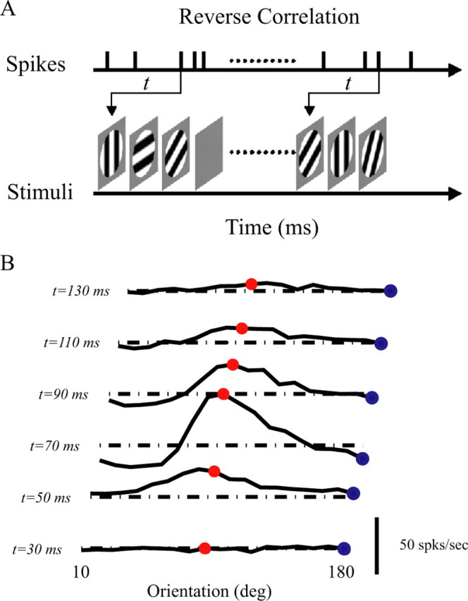
Dynamic orientation tuning measured by reverse correlation. A, The reverse correlation method. Stimuli with different orientations plus a blank were flashed for 20 ms in a random sequence. The spike time of each cell was recorded with 1 ms resolution. B, Dynamics of orientation tuning of an example cell. Tuning curves are plotted every 20 ms, starting at 30 ms after stimulus onset and ending at 130 ms after stimulus onset. The red points represent the responses of cells to orientation at 90° (preferred orientation) and blue points are the responses of cells to orientation at 180° (orthogonal to preferred). For convenience, the tuning curves of each cell were shifted by a fixed value, so that its preferred orientation is ∼90°. The dash-dot lines in B represent the responses of cells to blank stimulus.

Each stimulus in a sequence was randomly chosen from the 152 types of stimuli with replacement and flashed to a cell for two refresh frames (20 ms). The length of a random sequence of the stimuli was 30 s for each trial. Thirty trials were run for each experiment; this took 15 min altogether. The sequences of the stimuli were saved in the computer, and the spike times of the cell were recorded with 1 ms resolution.

Orientation tuning curves measured with drifting gratings

In the present experiments, we measured conventional orientation-tuning curves with drifting gratings as stimuli (Ringach et al., 2002b; Xing et al., 2004). Orientation was varied over a range of 360° in steps of 20° or less for grating stimuli of the optimal spatial and temporal frequency. The contrast was 0.8.

Orientation bandwidth.

Given the orientation tuning curve of a cell, we smoothed the curve with a Hanning window filter whose width is 18° (Ringach et al., 2002b; Xing et al., 2004). Then we found the peak response (R_pref) in the smoothed curve; its orientation was defined as the preferred orientation. Then we found the points on both sides of the peak at which the responses of the cell were just one-half of the peak response. One-half of the distance between the two points is the orientation bandwidth.

Ratio (O/P) of R_orth and R_pref.

On the smoothed orientation tuning curve, we found out the responses of a cell to the orientation 90° on either side of its preferred orientation. R_orth was defined as the mean of these two responses. As one measure of orientation selectivity, we computed the ratio R_orth/R_pref, which is referred to throughout this paper as the O/P ratio.

Results

We ran experiments on 140 extracellularly recorded macaque V1 cells with two different sets of stimuli: (1) briefly flashed gratings (for reverse correlation in the orientation domain; Fig. 1) and (2) drifting gratings. Orientation tuning curves were measured with both types of stimuli at high (0.8) contrast. For each neuron, the stimuli were all of optimal size for producing the largest response. For each cell, the optimum spatial frequency was determined using drifting gratings, and then that spatial frequency was used for both drifting and flashed stimuli.

The overall goal of the study was to estimate how much untuned suppression contributes to orientation tuning measured with drifting grating stimuli (Fig. 2). For many neurons that have no spontaneous firing rate, it is not possible to measure how much gratings at nonpreferred orientation suppress the extracellularly recorded spiking response. Using reverse correlation with dynamically presented gratings (Fig. 1), we measured untuned suppression even in cells with low spontaneous firing rates [because the rapid stimulus stream used to measure reverse correlation (Fig. 1A) causes an elevation of mean spike rate above the spontaneous firing rate in all V1 neurons we studied]. We characterized a threshold-power law model for each cell by a procedure similar to that introduced by Ringach and Malone (2007); we compared the measured firing rate with the predicted firing rate from the first-order response (spike-triggered average). Nonlinear deviations from the first-order prediction defined the threshold-power law model. The next step was to sum the dynamic responses over time and feed the time-integrated response to the threshold-power law model (Fig. 2). The predictions of the model matched the orientation selectivity of drifting grating responses well, as documented below, establishing a link between reverse correlation and drifting grating orientation tuning. Finally, the untuned suppression estimate for each single neuron was subtracted from the dynamics and then the drifting grating response recalculated with the threshold-power law model (Fig. 2). Comparison of orientation selectivity with and without untuned suppression on a neuron-by-neuron basis provided a quantitative estimate of how much untuned suppression contributed to selectivity across the entire population of V1 cells (Fig. 2).

Figure 2.

Plan of experiments. Using reverse correlation with dynamically presented gratings (Fig. 1), we estimated tuned enhancement and untuned suppression (Fig. 4). Next, we summed the dynamic responses over time and fed the integrated response in to a threshold-rate model. Finally, the untuned suppression estimate for each single neuron was subtracted from the dynamics and then the drifting grating response recalculated. Comparison of orientation selectivity with and without untuned suppression provided quantitative estimates of how much untuned suppression contributed to selectivity on a neuron-by-neuron basis.

Orientation dynamics and reverse correlation

The dynamics of orientation selectivity were measured by reverse correlation as diagrammed in Figure 1A (for details, see Materials and Methods). Figure 1B shows the dynamics of orientation selectivity of a typical cell. The reverse correlation procedure calculates the probability p(θ,τ) that a spike was caused by a grating of orientation angle θ at the time τ ms preceding the spike. To make a comparison of dynamic data and drifting-grating data, in this study, we used as a measure of neural response the firing rate that is proportional to p(θ,τ), instead of the log form used in previous papers. We defined the response of a cell to orientation θ at time delay τ ms as R_rvc(θ,τ) = (p(θ,τ) − p(blank, τ))*1000, where the subscript “rvc” indicates this is the response derived from the reverse correlation experiment. The blank response probability p(blank, τ) had its own time course that defined the response of the neuron to a blank coming in the input stream of other visual images. The response of a cell to a blank stimulus served as a baseline; R_rvc(blank,τ) was mapped to zero (Fig. 1B, dashed lines). R_rvc(θ,τ) being negative is a sign of suppression because it means that the grating of orientation θ evoked fewer spikes than a blank screen did.

Population averages of the time course of reverse correlation responses at preferred and orthogonal orientations (Fig. 3A) illustrate why the existence of untuned suppression is needed to explain orientation selectivity (Ringach et al., 2003; Xing et al., 2005). The reverse correlation response at the orthogonal-to-preferred orientation, R_rvc(θ_pref + 90, τ) was called R_orth(τ). R_orth(τ) was usually biphasic while the response at the preferred orientation, R_rvc(θ_pref,τ), called R_pref(τ), was usually monophasic, as graphed in Figure 3A. The population averages graphed in Figure 3A indicate that the differences in response time course between R_pref(τ) and R_orth(τ) were robust. The difference in response dynamics can be explained by untuned suppression as shown below.

Figure 3.

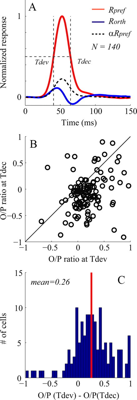
Dynamic responses in V1. A, Population averaged dynamic responses to their preferred orientations (R_pref, red curve) compared with dynamic responses to their orthogonal orientations (R_orth, blue curve) for V1 cells. The dashed curve is a rescaled version of R_pref by α (=0.27) to match the early part of R_orth. The intersections of vertical lines and horizontal line represent T_dev and T_dec. B, Scatter plot of O/P ratio (ratio of R_orth to R_pref) for individual V1 cells, at T_dev and T_dec. C, The distribution of the difference of O/P ratio between T_dev and T_dec. In C, the red vertical line represents the mean difference of O/P.

Another way of seeing the effect of untuned suppression is to compare the shapes of the orientation tuning curves of early with late responses. This comparison is illustrated in Figure 3, B and C. The O/P ratio = R_orth/R_pref was calculated at the two times at which R_pref (τ) = 1/2 R_pref (τ_peak); the two times were τ_dev on the rising (or developing) phase of the response and τ_dec later, on the falling (or declining) phase (Fig. 3A) and τ_peak represents the time when R_pref reaches its peak value. If the only visually driven input to the cortical cell were excitation, the orthogonal response time course would simply be a rescaled version of the response time course at the preferred orientation, graphed in Figure 3A as the dashed curve. Then the O/P ratio at τ_dev would be the same as at τ_dec. But the O/P ratio was usually smaller (indicating greater selectivity) at τ_dec than at τ_dev (Fig. 3B,C). One can explain both the biphasic time course of R_orth(τ) (Fig. 3A) and the lower O/P ratio at τ_dec (Fig. 3B,C) as consequences of the time course of untuned suppression being slightly slower than that of excitation, causing later responses to be more suppressed than earlier responses.

Modeling dynamic orientation tuning and estimating untuned suppression

To estimate the strength and time course of suppression, we used a simplified version of the three-component (tuned enhancement, untuned suppression, and tuned suppression) model devised previously to account for V1 orientation dynamics (below, Eq. 2) (Ringach et al., 2003; Xing et al., 2005). The orientation dynamics of a V1 cell had strong tuned enhancement [E(θ,τ) in Eq. 2] and untuned suppression [U(τ) in Eq. 2] but usually negligibly small tuned suppression [T(θ,τ) in the study by Xing et al. (2005), but ignored here] when the stimulus was of optimal size (Xing et al., 2005), as in the experiments done here. Therefore, in this paper, we used a simpler two-component model.

We assumed that the dynamics of orientation tuning were controlled only by an excitatory process we called tuned enhancement E(θ,τ) that was a function of orientation and time, and by untuned suppression U(τ) defined to be independent of orientation. As in the study by Xing et al. (2005), we made the approximation that tuned enhancement E(θ,τ) was separable in orientation and time (i.e., the product of an orientation tuning curve and a time dependence) as follows:

In other words, the orientation-tuning curve of excitation was assumed to be independent of time. This is an approximation that is based on results in the studies by Sharon and Grinvald (2002) and Anderson et al. (2000). As in the study by Xing et al. (2005), this approximation was validated by the good fit of the descriptive model to the dynamics data. The mean fractional error of this approximation of orientation-time separability on average across the V1 population was 0.04 for the fitting at optimal stimulus size (Xing et al., 2005). We defined the ratio of the excitatory responses at the orthogonal to preferred orientations as α = E_θ (θ_orth)/E_θ (θ_pref); α could be calculated from the measured orthogonal/preferred response ratio at short times <40 ms (Xing et al., 2005).

The simplified model is written in Equation 2. The simplified model contained the assumption that tuned suppression T(θ,τ) ≈ 0. Therefore, the reverse correlation response was modeled simply as the difference between excitation and untuned suppression.

The measurable responses R_pref(τ) and R_orth(τ) were expressed in terms of excitation and untuned suppression in Equations 3 and 4, by following Equation 2, and substituting the rescaled E(θ_pref,τ) for E(θ_orth,τ). Then algebraic rearrangement led to Equation 5, which expresses U(τ) in terms of R_pref(τ) and R_orth(τ) as follows:

Equation 5 was used to estimate untuned suppression for each cell. In Figure 4, the estimation procedure is illustrated with orientation dynamics data of one representative V1 cell. Time courses of R_pref(τ), R_orth(τ), and αR_pref(τ) are depicted in Figure 4A. The dashed curve in Figure 4A is αR_pref(τ) and the blue solid curve is R_orth(τ). From Equation 5, U(τ), graphed in Figure 4B, was proportional to the difference αR_pref(τ) − R_orth(τ). The population distribution of the estimated peak values of U(τ) for all the cells in the population is graphed in Figure 4C.

Figure 4.

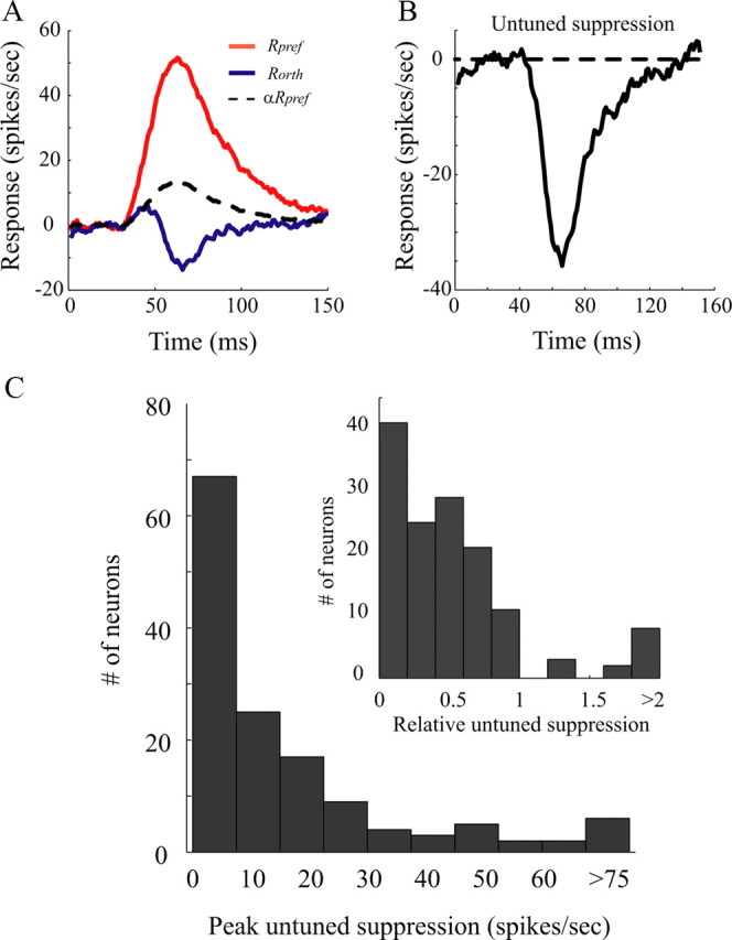
Untuned suppression is needed to model the dynamic orientation tuning for individual V1 cells. A shows the time courses of R_pref (red curves) and R_orth (blue curves) from a V1 cell. Both R_orth and R_pref have positive responses at early time. At early time (before 45 ms after stimulus onset), R_orth has a time course similar to R_pref but is rescaled by α, 0.48 (dashed curve). At later times, the blue and dashed curves are different because of untuned suppression. B shows estimated untuned suppression for this cell. C, Population distribution of the estimated peak values of U(t) for all the cells in the population. The inset shows the distribution of the peak untuned suppression relative to the peak response to the preferred orientation.

Prediction of drifting grating responses from orientation dynamics: operating point analysis

Next, we linked the dynamic orientation-tuning of each cell and its orientation tuning for drifting gratings. The link between the drifting-grating response R_dg and reverse correlation response is described by time averaging (Eq. 6) and a threshold-power law model (Eq. 7) as follows:

We developed a procedure for estimating the threshold and power law parameters inspired by the results about cell operating points in the study by Ringach and Malone (2007). The reverse-correlation response R_rvc(θ,t) was averaged over 140 ms in Equation 6. The time over which the response was averaged was chosen as 140 ms because empirically all V1 response dynamics relaxed back to zero by then. Averaging over a longer time, say up to the period of the drifting grating stimulus, would yield no more stimulus-dependent response. The mean firing rate of each experiment (MR_rvc) then was used to normalize the responses in Equation 6 to make the averaged response dimensionless. Then the drifting grating response was predicted by Equation 7, which describes a nonlinear threshold-power law model of a cortical cell. It is worth noting that the threshold parameter Th is the estimated distance between cell membrane potential and spike-firing threshold during the RVC experiment.

The parameters of the threshold-power law function in Equation 7 of each cell were estimated based on the idea that the responses to drifting gratings would be affected by the same spike-threshold and power law nonlinearity as affected the responses in the reverse correlation experiment. Support for this idea comes from the experimental fact that the mean firing rate in the reverse correlation experiments was roughly the same as that in the drifting grating experiments (averaged across all orientations). The estimation procedure compared measured firing rates in the reverse correlation experiment with what one would predict from a linear model—the functional relation between measured rate and predicted rate would define the nonlinear response function of the cell (Ringach and Malone, 2007; Benucci et al., 2009). Therefore, for each cell studied we did the following: (1) We first made a linear prediction of the instantaneous firing rates of a neuron over 140 ms time windows as a function of time during a reverse correlation experiment, by filtering the stimulus time series with the first-order kernels of the neuron, R_rvc(θ,τ); (2) the measured instantaneous firing rates of the cell were averaged over 140 ms time windows throughout the response to the same reverse correlation stimulus; (3) the predicted firing rates then were ranked by their values from lowest to highest, and every 30 values in the ascending sequence were averaged, and the measured responses for the corresponding times were similarly averaged (just to get a better signal-to-noise estimate of the responses); and then (4) a scatter plot (Fig. 5A) was drawn where the coordinates of each point in the scatter plot were the linear prediction from step 1 above, averaged as in step 3, versus measured response from step 2 also averaged as in step 3; finally, (5) best fit values of scale factor (K), exponent (n), and threshold (Th) were calculated to give the best fit of Equation 7 to the scatter plot. For example, for the V1 neuron in Figure 5, K = 248 spikes/s, Th = −0.19, and n = 1.6.

Figure 5.

Estimation of the operating point of a representative V1 cell and a comparison of measured and predicted orientation tuning. A, The operating point of the V1 cell. The red curve is fitted by a power law K〈R_rvc(θ) − Th〉ⁿ (K = 248 spikes/s, Th = −0.19, and n = 1.6). B, The distribution of the exponent n of the power law for all V1 cells. C, The distribution of threshold Th for all V1 cells.

The distributions of the obtained values of n and Th across the V1 population are graphed in Figure 5, B and C. Across the population, the average values of the best-fitting parameter values were K = 126 spikes/s, n = 1.68 (Fig. 5B), and Th = −0.18 (Fig. 5C). The implication of these parameter values is that, during the reverse correlation experiments, V1 cells were acting in an approximately linear manner and their firing rates were above zero (this is the meaning of the negative threshold).

Having obtained the needed values of K, Th, and n, and using Equations 6 and 7, we then predicted for each cell its orientation tuning curve for drifting gratings. For each orientation θ, we first summed the first-order dynamic response to that orientation over the first 140 ms after stimulus onset (Eq. 6). Then we transformed this value by the threshold-power law function (Eq. 7) with the best-fit parameters for each cell. For example, for the representative cell in Figure 5A, such tuning curves are shown in Figure 7A. One might expect that, if the membrane potential of a cell were far below spike firing threshold in the drifting grating experiment, the measured orientation selectivity would be greater than that of the predicted tuning curve because of the iceberg effect (Priebe and Ferster, 2006; Finn et al., 2007). Good agreement between predicted and measured orientation selectivity would suggest the opposite, that the membrane potential of the cell was not far below spike-firing threshold during the drifting grating experiments.

Figure 7.

Orientation tuning predicted by dynamic responses versus those measured by drifting gratings. A, An example of a single neuron (the same neuron as in Fig. 5A). The orientation tuning curve of the cell predicted from the power law function derived from Figure 5A. B, For the same V1 cell, the orientation tuning curve was also measured by drifting gratings. The dashed line in B represents the spontaneous firing rate. C, Scatter plot of the predicted orientation bandwidths of V1 cells (x-axis) versus those measured by drifting gratings (y-axis). D, Comparison of predicted versus measured O/P ratio shown by a scatter plot of O/P ratio predicted by reverse correlation experiments (x-axis) and O/P ratio measured with drifting gratings (y-axis). Correlation coefficients were as follows: 0.73 for bandwidth, 0.91 for O/P ratio.

Comparing tuning curves to drifting versus rapidly flashed gratings

One test of the agreement between the predictions of the threshold-power law model and drifting grating measurements is a comparison of the measured peak spike rate in the drifting grating experiment with the predicted peak spike rate from the threshold-power law model. This comparison is shown in Figure 6A. The predicted and measured firing rate peaks span the same range and are highly correlated (r = 0.68). This is a highly nontrivial result that depends on an accurate measurement of the reverse correlation response, on temporal integration of the dynamic response (Eq. 6) and on the accurate estimation of parameters of the threshold-power law model (Eq. 7). Empirical justification that temporal integration is required is shown in Figure 6B where the peak response to the drifting grating stimulus is plotted in a scatter plot versus the peak response of the reverse correlation. The points are much further from the identity line in Figure 6B than in Figure 6A, because temporal integration was not taken into account in Figure 6B. Empirical evidence that the threshold-power law is needed is shown in Figure 6C, which is a scatter plot: {Peak response (dynamic)/Peak response (drifting)} plotted on a logarithmic axis versus the power law exponent n. There is little correlation between log ratio and exponent (correlation coefficient r = −0.23). This means that the exponent is independent information about the operating point nonlinearity of the cortical cell.

Figure 6.

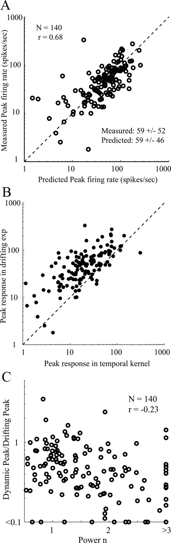
Peak firing rates predicted by dynamic responses versus those measured by drifting gratings. A, Scatter plot of the predicted peak firing rates of V1 cells (x-axis) versus those measured by drifting gratings (y-axis). The predicted and measured rates are highly correlated (r = 0.68). B, Scatter plot of the measured peak firing rates of V1 cells measured by drifting gratings (x-axis) versus peak responses measured by reverse correlation experiments (y-axis). C, Scatter plot of the estimated power n of V1 cells (x-axis) versus ratio of peak responses measured by reverse correlation experiments and drifting grating experiments. The dashed lines in A and B represent identity lines.

To support more fully the idea that the power law model allowed us to link the dynamics experiments with the drifting grating experiments, we briefly present a comparison of predicted orientation selectivity (Fig. 7A for an example neuron) and orientation selectivity measured by drifting gratings (Fig. 7B for the same example neuron) across the V1 population. Both orientation bandwidths [Fig. 7C, where we only include the 109 cells with orthogonal/preferred (O/P) ratio <0.5] and O/P ratio (Fig. 7D) were highly correlated between predicted and measured orientation tuning from responses to drifting gratings. The correlation coefficient for bandwidth was 0.73, while the correlation coefficient for O/P ratio was 0.91. Nishimoto et al. (2005) did a similar analysis for orientation bandwidth in cat area 17 cells, with a similar good agreement between dynamic and drifting-grating bandwidths. If instead of fitting the threshold-power law model, we simply made a linear prediction based on the time-integrated R_rvc, we also obtained good agreement between predicted and measured orientation bandwidth (r = 0.60; N = 109) and O/P ratio (r = 0.67; N = 140), although the correlation coefficients were smaller than those obtained with the threshold-power law model.

How untuned suppression affects steady-state orientation tuning

Finally, we used the dynamic measurements to assess the contribution of untuned suppression to orientation selectivity. Across the population of V1 neurons we performed an analysis on a cell-by-cell basis as follows: (1) first, we estimated untuned suppression from the orientation dynamics of an individual cell (Fig. 4); (2) we then computed the orientation tuning of the cell for drifting gratings based on the threshold-power law model described in the previous section of Results (Eqs. 6, 7; Figs. 5, 7); (3) finally, we computed from the threshold-power law model what the orientation tuning of the cell for drifting gratings should be when its untuned suppression was removed, by using a modified R_rvc(θ) with untuned suppression set equal to zero.

The results of the analysis are displayed in Figure 8. In the left-hand column, the results are shown as frequency histograms of O/P ratio. The distribution of O/P ratio, measured by drifting gratings, is positively skewed with a long tail (Fig. 8A). This is very similar to the distribution of O/P ratios predicted from dynamic orientation tuning (Kolmogorov–Smirnov test, p = 0.37; Fig. 8B). However, when untuned suppression was removed, the number of cells predicted to have an O/P ratio <0.2 dropped from 75 of 140 to 38 of 140, and the distribution of O/P ratio became significantly less skewed and flatter (Kolmogorov–Smirnov test, p < 0.001; Fig. 8C). The cell-by-cell change in O/P ratio is illustrated in the scatter plot in Figure 8D. Nearly all cells (average change of O/P ratio is 0.12; p < 0.001, t test for pair sample) showed a positive change of O/P ratio with removal of untuned suppression (Fig. 8D, points above the diagonal line), indicating that the effect of untuned suppression on the responses of V1 cells to nonoptimal orientations is general across the population.

Figure 8.

The effect of untuned suppression on O/P ratio estimated across the V1 population. A, Distribution of the measured O/P ratio of V1 cells from experiments with drifting gratings as stimuli. B, Distribution of the O/P ratio of V1 cells estimated from dynamics experiments that include untuned suppression. C, Distribution of the O/P ratio of V1 cells without untuned suppression, estimated from dynamics experiments. D, A scatter plot for N = 140 cells recorded in V1 of predicted O/P ratio (x-axis) versus O/P ratio without untuned suppression (y-axis). The distance of each point from the unit line, drawn as the diagonal, is the amount untuned suppression contributed to orientation selectivity.

Untuned suppression increases orientation selectivity by reducing the vertical offset of the orientation tuning curves. This is illustrated for a single representative V1 neuron and for the V1 population in Figure 9. Figure 9, A and B, shows the change of the orientation tuning of one cell due to its untuned suppression. When we removed the effect of untuned suppression, the whole orientation tuning curve (Fig. 9B) shifted upward by the amount of untuned suppression, decreasing the relative difference between responses at preferred and orthogonal orientations. This effect can also be seen in the population average in Figure 9C.

Figure 9.

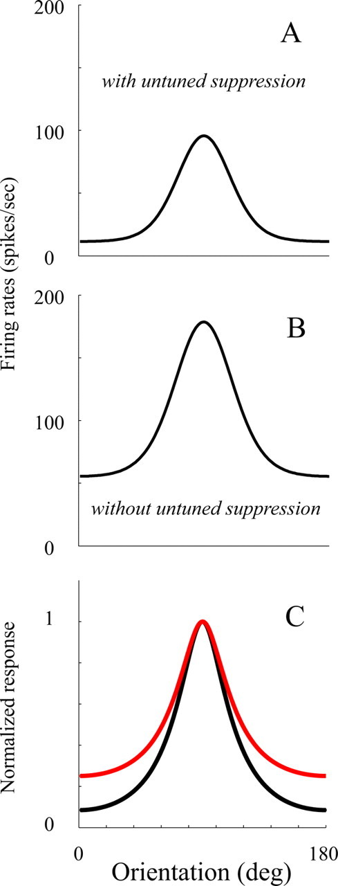
Change of orientation tuning curves with removal of untuned suppression. A and B show the change of the orientation tuning curve of an example cell, before and after its untuned suppression was removed. C, The population (cells with O/P < 0.2) averaged orientation tuning (black curve; O/P = 0.08) compared with the population average orientation tuning without untuned suppression (red curve; O/P = 0.25).

It is especially noticeable that many sharply tuned cells (O/P < 0.2) are strongly affected by the removal of untuned suppression (Fig. 8D). The largest increase of O/P ratio as a result of the removal of untuned suppression happens to cells with an original O/P ratio <0.2 (Fig. 9). On average, untuned suppression reduces the O/P ratio for these cells from 0.25 to 0.08. This suggests that the most highly selective cells are greatly affected by untuned suppression (changes of O/P ratio are 0.17 for neurons with O/P ratio <0.2 and 0.12 for the whole population). Overall, the results suggest that the receptive fields of neurons with high orientation selectivity are not just formed by their excitatory input but that untuned suppression plays an important role in increasing the orientation selectivities of these cells.

Weakly tuned “untuned suppression”

Suppose cortical inhibition does not produce untuned suppression but weakly tuned suppression as predicted by models (McLaughlin et al., 2000; Mariño et al., 2005). Here, we show how the estimation of the suppression controlling R_orth, and the estimation of contribution of this process to orientation selectivity are affected, if suppression is not completely untuned. If the suppressive process controlling R_orth has similar orientation preference and bandwidth (without offset) as excitatory processes, we can divide this suppressive process into two parts, U(τ) and u(θ,τ) so that u(θ,τ) is always proportional (with a constant of proportionality k, 0 < k < 1) to E(θ,τ) at each time delay τ, as shown in Equations 2′, 3′, and 4′ as follows:

Then we can only estimate U(τ) (shown in Eq. 5′) and will miss the u(θ,τ) part, which is hidden in E(θ,τ).

Discussion

Our experimental results and analysis provide the first quantitative estimates of the contribution of untuned suppression to orientation selectivity. Untuned suppression made a significant quantitative contribution to the orientation selectivity of V1 cells by attenuating responses to nonpreferred stimuli.

Neuronal processes involved in orientation selectivity

One of the main problems the visual cortex needs to solve, to generate orientation selectivity, is the reduction of responses to nonpreferred orientations particularly when stimuli are high contrast (Ben-Yishai et al., 1995; Sompolinsky and Shapley, 1997; Troyer et al., 1998). Information theory analysis by Kang et al. (2004) showed that a pedestal of response to nonpreferred orientations degrades orientation discrimination by the V1 population. The original feedforward model provided by Hubel and Wiesel (1962) provides the bias for the preferred orientation in most cortical models. However, feedforward excitation alone cannot provide the suppression of responses to nonpreferred orientations that has been observed (De Valois et al., 1982; Celebrini et al., 1993; Ringach et al., 2002b).

To account for orientation selectivity, theorists have proposed corticocortical amplification (Ben-Yishai et al., 1995; Somers et al., 1995; Mariño et al., 2005), corticocortical inhibition (Sato et al., 1996; Troyer et al., 1998; McLaughlin et al., 2000; Monier et al., 2003), and presynaptic depression (Carandini et al., 2002; Freeman et al., 2002). Many experimental studies (Nelson and Frost, 1978; Sillito et al., 1980; Bonds, 1989; Volgushev et al., 1993; Sato et al., 1996; Ringach et al., 2002a,b; Shapley et al., 2003) concluded that suppressive or inhibitory cortical mechanisms were involved. However, more recent studies (Carandini et al., 2002; Freeman et al., 2002; Priebe and Ferster, 2006; Finn et al., 2007; Koelling et al., 2008) suggested that the suppressive effects studied earlier in experiments that used plaids and drifting gratings as stimuli might be due to nonlinearities in the retina and/or LGN. These reexaminations of the neuronal mechanism of orientation selectivity motivated us to make a quantitative assessment of the contribution of untuned suppression.

The role of untuned suppression

The existence of untuned suppression is consistent with theoretical studies that suggest that local cortical inhibition generates broadly tuned (or untuned) suppression (Troyer et al., 1998; McLaughlin et al., 2000). Intracellular measurements in cat V1 prove the existence of broadly tuned cortical inhibition (Volgushev et al., 1993; Anderson et al., 2000; Gillespie et al., 2001; Monier et al., 2003). Studies in cat (Nowak et al., 2008) and mouse (Niell and Stryker, 2008) cortex indicate that there is a subgroup of fast-spiking V1 neurons, presumed inhibitory interneurons, that are untuned or poorly tuned for orientation. Additional evidence comes from the study by Sato et al. (1996), in which cortical GABAergic inhibition in macaque V1 was weakened by bicuculline.

Thresholds, power laws, and operating points

Spike-firing threshold has been considered as another possible mechanism for high orientation selectivity in responses to drifting grating patterns (Jones et al., 1987; Gardner et al., 1999). The spiking threshold acting as an iceberg effect (Rose and Blakemore, 1974) is unlikely to account for orientation selectivity (Sompolinsky and Shapley, 1997; Troyer et al., 1998), but more recent work (Priebe and Ferster, 2006; Finn et al., 2007) proposed a more sophisticated model regarding spike-firing threshold. In this model, the spike-firing threshold makes a visual cortical neuron transform its membrane potential into cycle-averaged firing rates like a power law transducer (Hansel and van Vreeswijk, 2002; Miller and Troyer, 2002). If the power law exponent were much larger than 1, the firing rate of the neuron would increase much more than proportionally to membrane potential and this would sharpen orientation tuning. Experimental results suggested that the exponent was between 2 and 3 (Anzai et al., 1999; Gardner et al., 1999; Finn et al., 2007). However, the good agreement we found between reverse correlation predictions and drifting grating data suggests rather that V1 neurons are not far below threshold and are not acting like power law transducers in our drifting grating experiments. The threshold-power law model we considered in Results was not about the nonlinearity of spike-threshold but rather characterized the amount of response in the RVC experiment that cannot be accounted for fully by the first-order kernel. The average exponent n of that model was low, ∼1.6. While Nishimoto et al. (2005) have pointed out that nonlinearities might be subsumed within the kernel estimation, there was no dependence of our estimation of the contribution of untuned suppression on exponent n (Fig. 10B).

Figure 10.

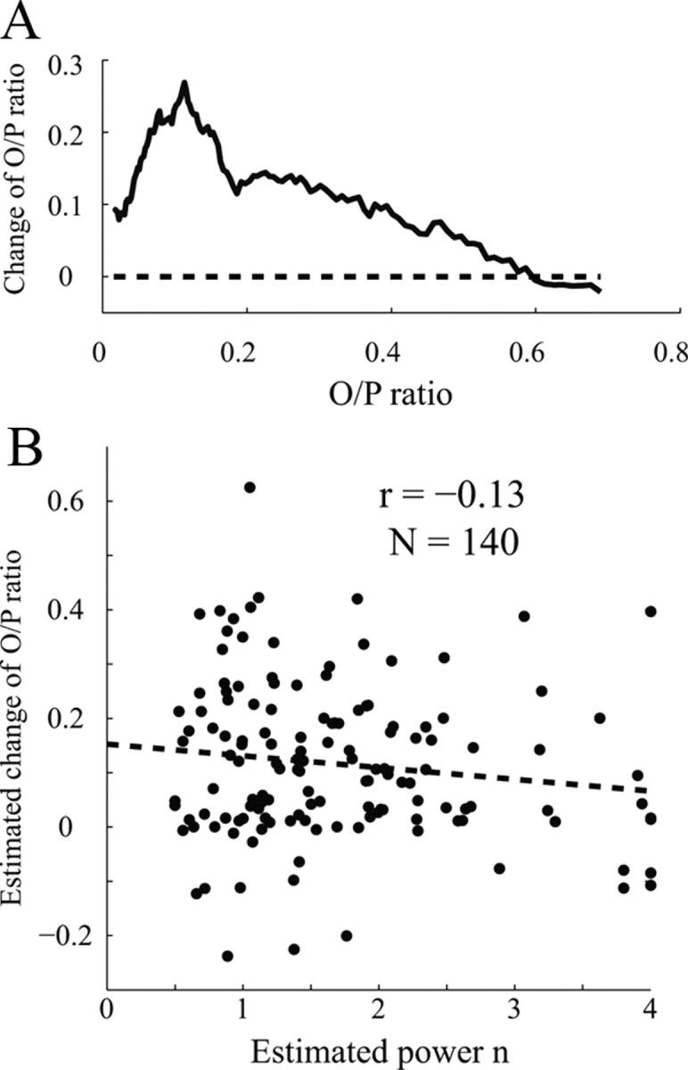
A, Untuned suppression has stronger effects on sharply tuned V1 cells. The graph shows the predicted change of O/P ratio caused by removing untuned suppression (y-axis) plotted versus the measured O/P ratio of V1 cells (x-axis). The biggest effects are at low O/P ratios (most highly selective cells). B, Untuned suppression is not significantly correlated to estimated exponent n in the V1 population. The graph shows the predicted change of O/P ratio caused by removing untuned suppression (y-axis) plotted versus the estimated exponent n of V1 cells (x-axis). The correlation is not significant (p = 0.125).

The challenge remains to reconcile results from different laboratories. One possibility is that cortices studied in different laboratories were at different operating points (Ringach and Malone, 2007). Perhaps the widely divergent estimates of the exponents of power law models may reflect different operating points caused by the use of different visual stimuli or different pharmacological treatments. Supporting evidence that the operating points of our experiments and those of Finn et al. (2007) were different comes from an analysis of the population distributions of spontaneous firing rate and O/P ratio, as follows.

The suggestion of different operating points is consistent with the difference in spontaneous firing rates in the populations of V1 cells reported by different laboratories. In our dataset, only 20% of cells have spontaneous firing rate = 0 (mean, 4.6 spikes/s; N = 480); among simple cells, 33% have spontaneous firing rate = 0 (mean, 2.4 spikes/s; N = 207). The spontaneous firing rates from our sufentanyl-anesthetized monkeys were somewhat lower than those observed in awake monkeys (Gur et al., 2005; Chen et al., 2009) (personal communication between Dr. Bruce Cumming and Dr. Michael J. Hawken) but still significantly above 0 spikes/s. However, Finn et al. (2007) suggested that most simple cells they recorded in cat V1 had zero spontaneous firing rates (inferred from the zero firing rates to nonpreferred orientations). Different experimental procedures in different laboratories could lead to different views of the effect of spike-firing threshold on orientation selectivity. When the threshold is high, it can improve orientation selectivity by preventing responses to nonpreferred orientations. The high threshold may hide inhibitory effects. However, when threshold is relatively low, untuned suppression is more obvious and is observed to have a stronger influence on orientation selectivity.

An indication of the different operating points in different experiments also can be seen in the distribution of O/P ratios measured from different laboratories. In our database, the distribution of O/P ratio peaked near zero and was positively skewed with a long tail to 1, as in Figure 7A. However, from the very low firing rates to nonpreferred orientations reported by Finn et al. (2007), it is reasonable to expect that the distribution of the O/P ratio of their population would have a peak at zero and little or no skewed tail above zero O/P. We conclude that our dataset is from V1 when its operating point is somewhat similar to that of the awake animal, and that the data of Finn et al. (2007) are from a visual cortex that is working at a different operating point.

Neuronal mechanism of untuned suppression

Previously, we found that a relatively slower tuned suppression is size dependent, but more rapid untuned suppression is the same for stimuli of optimal size and for stimuli two to four times larger (Xing et al., 2005). Such size invariance of untuned suppression suggests that it is a process mainly due to local circuitry in V1. In our descriptive model, untuned suppression is constant as a function of orientation. However, McLaughlin et al. (2000) and Mariño et al. (2005) using computational models of V1 have suggested that the inhibitory effect on a V1 cell due to local circuitry may in some cases be tuned with a bandwidth similar to tuned excitation but with a much larger orthogonal/preferred (O/P) ratio than feedforward and local circuit excitation. If these models were correct and the inhibitory tuning and excitatory tuning were similar around the peak of the tuning curve, we would be unable to dissect the tuned part of the local suppression process from excitation using the curve-fitting procedure we used with our three-component model. So even though in our simplified model the suppressive process controlling R_orth is flat, we do not exclude the possibility that the suppressive process controlling R_orth is also tuned with similar orientation preference and bandwidth as enhancement. But the inhibitory process must have a pedestal of suppression across all orientations to be compatible with the dynamics data. If untuned suppression in our model is indeed broadly tuned as described above, our model will tend to underestimate the total amount of suppression, but the estimation of contribution of the untuned suppression—the untuned portion of the suppressive process—will be unaffected (as shown at end of Results).

Untuned suppression appears to be a cortical process. Untuned suppression is too slow to be a retinal or LGN effect, but too rapidly decaying to be consistent with synaptic depression at thalamocortical or corticocortical synapses. Synaptic depression is also ruled out as an explanation from the results of Boudreau and Ferster (2005). The neuropharmacological results of Sato et al. (1996) support the idea that cortical GABAergic inhibition is the source of untuned suppression since it can be blocked by bicuculline applied in the cortex.

References

- Anderson JS, Carandini M, Ferster D. Orientation tuning of input conductance, excitation, and inhibition in cat primary visual cortex. J Neurophysiol. 2000;84:909–926. doi: 10.1152/jn.2000.84.2.909. [DOI] [PubMed] [Google Scholar]
- Anzai A, Ohzawa I, Freeman RD. Neural mechanisms for processing binocular information. I. Simple cells. J Neurophysiol. 1999;82:891–908. doi: 10.1152/jn.1999.82.2.891. [DOI] [PubMed] [Google Scholar]
- Benucci A, Ringach DL, Carandini M. Coding of stimulus sequences by population responses in visual cortex. Nat Neurosci. 2009;12:1317–1324. doi: 10.1038/nn.2398. [DOI] [PMC free article] [PubMed] [Google Scholar]
- Ben-Yishai R, Bar-Or RL, Sompolinsky H. Theory of orientation tuning in visual cortex. Proc Natl Acad Sci U S A. 1995;92:3844–3848. doi: 10.1073/pnas.92.9.3844. [DOI] [PMC free article] [PubMed] [Google Scholar]
- Bonds AB. Role of inhibition in the specification of orientation selectivity of cells in the cat striate cortex. Vis Neurosci. 1989;2:41–55. doi: 10.1017/s0952523800004314. [DOI] [PubMed] [Google Scholar]
- Boudreau CE, Ferster D. Short-term depression in thalamocortical synapses of cat primary visual cortex. J Neurosci. 2005;25:7179–7190. doi: 10.1523/JNEUROSCI.1445-05.2005. [DOI] [PMC free article] [PubMed] [Google Scholar]
- Carandini M, Heeger DJ, Senn W. A synaptic explanation of suppression in visual cortex. J Neurosci. 2002;22:10053–10065. doi: 10.1523/JNEUROSCI.22-22-10053.2002. [DOI] [PMC free article] [PubMed] [Google Scholar]
- Celebrini S, Thorpe S, Trotter Y, Imbert M. Dynamics of orientation coding in area V1 of the awake primate. Vis Neurosci. 1993;10:811–825. doi: 10.1017/s0952523800006052. [DOI] [PubMed] [Google Scholar]
- Chen Y, Anand S, Martinez-Conde S, Macknik SL, Bereshpolova Y, Swadlow HA, Alonso JM. The linearity and selectivity of neuronal responses in awake visual cortex. J Vis. 2009;9:12.1–17. doi: 10.1167/9.9.12. [DOI] [PMC free article] [PubMed] [Google Scholar]
- Curtis JC, Kleinfeld D. Phase-to-rate transformations encode touch in cortical neurons of a scanning sensorimotor system. Nat Neurosci. 2009;12:492–501. doi: 10.1038/nn.2283. [DOI] [PMC free article] [PubMed] [Google Scholar]
- De Valois RL, Yund EW, Hepler N. The orientation and direction selectivity of cells in macaque visual cortex. Vision Res. 1982;22:531–544. doi: 10.1016/0042-6989(82)90112-2. [DOI] [PubMed] [Google Scholar]
- Finn IM, Priebe NJ, Ferster D. The emergence of contrast-invariant orientation tuning in simple cells of cat visual cortex. Neuron. 2007;54:137–152. doi: 10.1016/j.neuron.2007.02.029. [DOI] [PMC free article] [PubMed] [Google Scholar]
- Freeman TC, Durand S, Kiper DC, Carandini M. Suppression without inhibition in visual cortex. Neuron. 2002;35:759–771. doi: 10.1016/s0896-6273(02)00819-x. [DOI] [PubMed] [Google Scholar]
- Gardner JL, Anzai A, Ohzawa I, Freeman RD. Linear and nonlinear contributions to orientation tuning of simple cells in the cat's striate cortex. Vis Neurosci. 1999;16:1115–1121. doi: 10.1017/s0952523899166112. [DOI] [PubMed] [Google Scholar]
- Gillespie DC, Lampl I, Anderson JS, Ferster D. Dynamics of the orientation-tuned membrane potential response in cat primary visual cortex. Nat Neurosci. 2001;4:1014–1019. doi: 10.1038/nn731. [DOI] [PubMed] [Google Scholar]
- Gur M, Kagan I, Snodderly DM. Orientation and direction selectivity of neurons in V1 of alert monkeys: functional relationships and laminar distributions. Cereb Cortex. 2005;15:1207–1221. doi: 10.1093/cercor/bhi003. [DOI] [PubMed] [Google Scholar]
- Hansel D, van Vreeswijk C. How noise contributes to contrast invariance of orientation tuning in cat visual cortex. J Neurosci. 2002;22:5118–5128. doi: 10.1523/JNEUROSCI.22-12-05118.2002. [DOI] [PMC free article] [PubMed] [Google Scholar]
- Hawken MJ, Shapley RM, Grosof DH. Temporal-frequency selectivity in monkey visual cortex. Vis Neurosci. 1996;13:477–492. doi: 10.1017/s0952523800008154. [DOI] [PubMed] [Google Scholar]
- Hubel DH, Wiesel TN. Receptive fields, binocular interaction and functional architecture in the cat's visual cortex. J Physiol. 1962;160:106–154. doi: 10.1113/jphysiol.1962.sp006837. [DOI] [PMC free article] [PubMed] [Google Scholar]
- Jones JP, Stepnoski A, Palmer LA. The two-dimensional spectral structure of simple receptive fields in cat striate cortex. J Neurophysiol. 1987;58:1212–1232. doi: 10.1152/jn.1987.58.6.1212. [DOI] [PubMed] [Google Scholar]
- Kang K, Shapley RM, Sompolinsky H. Information tuning of populations of neurons in primary visual cortex. J Neurosci. 2004;24:3726–3735. doi: 10.1523/JNEUROSCI.4272-03.2004. [DOI] [PMC free article] [PubMed] [Google Scholar]
- Koelling M, Shapley R, Shelley M. Retinal and cortical nonlinearities combine to produce masking in V1 responses to plaids. J Comput Neurosci. 2008;25:390–400. doi: 10.1007/s10827-008-0086-6. [DOI] [PubMed] [Google Scholar]
- Mariño J, Schummers J, Lyon DC, Schwabe L, Beck O, Wiesing P, Obermayer K, Sur M. Invariant computations in local cortical networks with balanced excitation and inhibition. Nat Neurosci. 2005;8:194–201. doi: 10.1038/nn1391. [DOI] [PubMed] [Google Scholar]
- McLaughlin D, Shapley R, Shelley M, Wielaard DJ. A neuronal network model of macaque primary visual cortex (V1): orientation selectivity and dynamics in the input layer 4Calpha. Proc Natl Acad Sci U S A. 2000;97:8087–8092. doi: 10.1073/pnas.110135097. [DOI] [PMC free article] [PubMed] [Google Scholar]
- Merchant H, Naselaris T, Georgopoulos AP. Dynamic sculpting of directional tuning in the primate motor cortex during three-dimensional reaching. J Neurosci. 2008;28:9164–9172. doi: 10.1523/JNEUROSCI.1898-08.2008. [DOI] [PMC free article] [PubMed] [Google Scholar]
- Miller KD, Troyer TW. Neural noise can explain expansive, power-law nonlinearities in neural response functions. J Neurophysiol. 2002;87:653–659. doi: 10.1152/jn.00425.2001. [DOI] [PubMed] [Google Scholar]
- Monier C, Chavane F, Baudot P, Graham LJ, Frégnac Y. Orientation and direction selectivity of synaptic inputs in visual cortical neurons: a diversity of combinations produces spike tuning. Neuron. 2003;37:663–680. doi: 10.1016/s0896-6273(03)00064-3. [DOI] [PubMed] [Google Scholar]
- Nelson JI, Frost BJ. Orientation-selective inhibition from beyond the classic visual receptive field. Brain Res. 1978;139:359–365. doi: 10.1016/0006-8993(78)90937-x. [DOI] [PubMed] [Google Scholar]
- Niell CM, Stryker MP. Highly selective receptive fields in mouse visual cortex. J Neurosci. 2008;28:7520–7536. doi: 10.1523/JNEUROSCI.0623-08.2008. [DOI] [PMC free article] [PubMed] [Google Scholar]
- Nishimoto S, Arai M, Ohzawa I. Accuracy of subspace mapping of spatiotemporal frequency domain visual receptive fields. J Neurophysiol. 2005;93:3524–3536. doi: 10.1152/jn.01169.2004. [DOI] [PubMed] [Google Scholar]
- Nowak LG, Sanchez-Vives MV, McCormick DA. Lack of orientation and direction selectivity in a subgroup of fast-spiking inhibitory interneurons: cellular and synaptic mechanisms and comparison with other electrophysiological cell types. Cereb Cortex. 2008;18:1058–1078. doi: 10.1093/cercor/bhm137. [DOI] [PMC free article] [PubMed] [Google Scholar]
- Priebe NJ, Ferster D. Mechanisms underlying cross-orientation suppression in cat visual cortex. Nat Neurosci. 2006;9:552–561. doi: 10.1038/nn1660. [DOI] [PubMed] [Google Scholar]
- Ringach DL, Malone BJ. The operating point of the cortex: neurons as large deviation detectors. J Neurosci. 2007;27:7673–7683. doi: 10.1523/JNEUROSCI.1048-07.2007. [DOI] [PMC free article] [PubMed] [Google Scholar]
- Ringach DL, Hawken MJ, Shapley R. Dynamics of orientation tuning in macaque primary visual cortex. Nature. 1997;387:281–284. doi: 10.1038/387281a0. [DOI] [PubMed] [Google Scholar]
- Ringach DL, Bredfeldt CE, Shapley RM, Hawken MJ. Suppression of neural responses to nonoptimal stimuli correlates with tuning selectivity in macaque V1. J Neurophysiol. 2002a;87:1018–1027. doi: 10.1152/jn.00614.2001. [DOI] [PubMed] [Google Scholar]
- Ringach DL, Shapley RM, Hawken MJ. Orientation selectivity in macaque V1: diversity and laminar dependence. J Neurosci. 2002b;22:5639–5651. doi: 10.1523/JNEUROSCI.22-13-05639.2002. [DOI] [PMC free article] [PubMed] [Google Scholar]
- Ringach DL, Hawken MJ, Shapley R. Dynamics of orientation tuning in macaque V1: the role of global and tuned suppression. J Neurophysiol. 2003;90:342–352. doi: 10.1152/jn.01018.2002. [DOI] [PubMed] [Google Scholar]
- Rose D, Blakemore C. Effects of bicuculline on functions of inhibition in visual cortex. Nature. 1974;249:375–377. doi: 10.1038/249375a0. [DOI] [PubMed] [Google Scholar]
- Sadagopan S, Wang X. Contribution of inhibition to stimulus selectivity in primary auditory cortex of awake primates. J Neurosci. 2010;30:7314–7325. doi: 10.1523/JNEUROSCI.5072-09.2010. [DOI] [PMC free article] [PubMed] [Google Scholar]
- Sato H, Katsuyama N, Tamura H, Hata Y, Tsumoto T. Mechanisms underlying orientation selectivity of neurons in the primary visual cortex of the macaque. J Physiol. 1996;494:757–771. doi: 10.1113/jphysiol.1996.sp021530. [DOI] [PMC free article] [PubMed] [Google Scholar]
- Sceniak MP, Ringach DL, Hawken MJ, Shapley R. Contrast's effect on spatial summation by macaque V1 neurons. Nat Neurosci. 1999;2:733–739. doi: 10.1038/11197. [DOI] [PubMed] [Google Scholar]
- Shapley R, Hawken M, Ringach DL. Dynamics of orientation selectivity in the primary visual cortex and the importance of cortical inhibition. Neuron. 2003;38:689–699. doi: 10.1016/s0896-6273(03)00332-5. [DOI] [PubMed] [Google Scholar]
- Sharon D, Grinvald A. Dynamics and constancy in cortical spatiotemporal patterns of orientation processing. Science. 2002;295:512–515. doi: 10.1126/science.1065916. [DOI] [PubMed] [Google Scholar]
- Sillito AM, Kemp JA, Milson JA, Berardi N. A re-evaluation of the mechanisms underlying simple cell orientation selectivity. Brain Res. 1980;194:517–520. doi: 10.1016/0006-8993(80)91234-2. [DOI] [PubMed] [Google Scholar]
- Somers DC, Nelson SB, Sur M. An emergent model of orientation selectivity in cat visual cortical simple cells. J Neurosci. 1995;15:5448–5465. doi: 10.1523/JNEUROSCI.15-08-05448.1995. [DOI] [PMC free article] [PubMed] [Google Scholar]
- Sompolinsky H, Shapley R. New perspectives on the mechanisms for orientation selectivity. Curr Opin Neurobiol. 1997;7:514–522. doi: 10.1016/s0959-4388(97)80031-1. [DOI] [PubMed] [Google Scholar]
- Troyer TW, Krukowski AE, Priebe NJ, Miller KD. Contrast-invariant orientation tuning in cat visual cortex: thalamocortical input tuning and correlation-based intracortical connectivity. J Neurosci. 1998;18:5908–5927. doi: 10.1523/JNEUROSCI.18-15-05908.1998. [DOI] [PMC free article] [PubMed] [Google Scholar]
- Volgushev M, Pei X, Vidyasagar TR, Creutzfeldt OD. Excitation and inhibition in orientation selectivity of cat visual cortex neurons revealed by whole-cell recordings in vivo. Vis Neurosci. 1993;10:1151–1155. doi: 10.1017/s0952523800010257. [DOI] [PubMed] [Google Scholar]
- Wu GK, Arbuckle R, Liu BH, Tao HW, Zhang LI. Lateral sharpening of cortical frequency tuning by approximately balanced inhibition. Neuron. 2008;58:132–143. doi: 10.1016/j.neuron.2008.01.035. [DOI] [PMC free article] [PubMed] [Google Scholar]
- Xing D, Ringach DL, Shapley R, Hawken MJ. Correlation of local and global orientation and spatial frequency tuning in macaque V1. J Physiol. 2004;557:923–933. doi: 10.1113/jphysiol.2004.062026. [DOI] [PMC free article] [PubMed] [Google Scholar]
- Xing D, Shapley RM, Hawken MJ, Ringach DL. Effect of stimulus size on the dynamics of orientation selectivity in macaque V1. J Neurophysiol. 2005;94:799–812. doi: 10.1152/jn.01139.2004. [DOI] [PubMed] [Google Scholar]