Cosine Directional Tuning of Theta Cell Burst Frequencies: Evidence for Spatial Coding by Oscillatory Interference

Abstract

The rodent septohippocampal system contains “theta cells,” which burst rhythmically at 4–12 Hz, but the functional significance of this rhythm remains poorly understood (Buzsáki, 2006). Theta rhythm commonly modulates the spike trains of spatially tuned neurons such as place (O'Keefe and Dostrovsky, 1971), head direction (Tsanov et al., 2011a), grid (Hafting et al., 2005), and border cells (Savelli et al., 2008; Solstad et al., 2008). An “oscillatory interference” theory has hypothesized that some of these spatially tuned neurons may derive their positional firing from phase interference among theta oscillations with frequencies that are modulated by the speed and direction of translational movements (Burgess et al., 2005, 2007). This theory is supported by studies reporting modulation of theta frequency by movement speed (Rivas et al., 1996; Geisler et al., 2007; Jeewajee et al., 2008a), but modulation of theta frequency by movement direction has never been observed. Here we recorded theta cells from hippocampus, medial septum, and anterior thalamus of freely behaving rats. Theta cell burst frequencies varied as the cosine of the rat's movement direction, and this directional tuning was influenced by landmark cues, in agreement with predictions of the oscillatory interference theory. Computer simulations and mathematical analysis demonstrated how a postsynaptic neuron can detect location-dependent synchrony among inputs from such theta cells, and thereby mimic the spatial tuning properties of place, grid, or border cells. These results suggest that theta cells may serve a high-level computational function by encoding a basis set of oscillatory signals that interfere with one another to synthesize spatial memory representations.

Introduction

The hippocampus and surrounding cortex contain neural circuits that store memories for facts and past experiences (Eichenbaum and Cohen, 1992; Squire and Schacter, 2002). In rodents, these regions contain neurons that fire selectively at preferred locations in space and might thus encode memories of familiar spatial environments (O'Keefe and Nadel, 1978; McNaughton et al., 2006). Several categories of spatially tuned neurons have been identified: place cells fire at one or a few preferred locations (O'Keefe and Dostrovsky, 1971), grid cells fire at multiple locations forming a hexagonal lattice (Hafting et al., 2005), and border cells fire in fixed relationships with environmental boundaries (Savelli et al., 2008; Solstad et al., 2008; Lever et al., 2009). These neurons are believed to participate in computing the animal's location by integrating its movement velocity over time, a process known as path integration (McNaughton et al., 1996; Etienne and Jeffery, 2004).

Spike trains of spatially tuned neurons are often modulated by 4–12 Hz theta oscillations, which have been proposed to play a key role in memory processing (O'Keefe and Recce, 1993; Buzsáki, 2006; Düzel et al., 2010; Hasselmo et al., 2010; Rutishauser et al., 2010; Bissiere et al., 2011). Burgess et al. (2005, 2007) introduced an “oscillatory interference” theory, hypothesizing that theta oscillations are generated by velocity-controlled oscillators (VCOs), which perform path integration by modulating their frequencies in proportion with the speed and direction of a rat's translational movements. Supporting this idea, theta frequency is indeed modulated by a rat's movement speed (Rivas et al., 1996; Geisler et al., 2007), and oscillatory properties of spatial neurons are correlated with their spatial tuning parameters in accordance with predictions of oscillatory interference models (Burgess et al., 2007; Giocomo et al., 2007; Jeewajee et al., 2008a; Zilli et al., 2009). However, oscillatory interference models explicitly require that VCO frequencies vary as the cosine of an animal's movement direction, and such directional modulation of theta oscillations has never been observed.

Here, rhythmically bursting theta cells were recorded from medial septum, hippocampus, and anterior thalamus in behaving rats. We found that burst frequencies of theta cells were modulated by the rat's movement direction with cosine-like tuning, and directional tuning functions followed rotations of landmark cues, suggesting that theta cells might encode VCO signals predicted by the oscillatory interference theory. Computer simulations revealed that a postsynaptic neuron could exhibit spatially selective firing by detecting location-dependent synchronization among inputs from theta cells with firing properties similar to those observed in our experiments. The postsynaptic neuron could mimic the firing rate maps not only of grid cells, as in prior oscillatory interference models (Burgess et al., 2007; Giocomo et al., 2007; Hasselmo et al., 2007; Burgess, 2008; Zilli and Hasselmo, 2010), but also of place and border cells. Based on these results, we propose how a network of central pattern generator (CPG) circuits composed exclusively from theta cells could provide a basis set of VCO signals for generating diverse populations of spatially tuned neurons such as place, grid, and border cells.

Materials and Methods

All experiments were conducted in accordance with the U.S. National Institute of Health Guide for the Care and Use of Laboratory Animals (NIH Publications No. 80-23), and were approved in advance by the animal subjects review committee at the University of California, Los Angeles. Technical descriptions of computer simulations and neurophysiological data analysis (including source code) are available on the ModelDB database (Hines et al., 2004) under accession number 129067 (http://senselab.med.yale.edu/modeldb/ShowModel.asp?model=129067).

Subjects and surgery.

Male Long–Evans rats weighing 350–400 g were housed singly and reduced to 85% of ad libitum weight through limited daily feeding, then trained over 5 d to forage for food pellets in an enclosed environment (see below, Recording sessions and behavior tracking). Under deep isoflurane anesthesia, rats were chronically implanted with tetrode arrays targeting medial septum and dorsal hippocampus (three rats) or anterior thalamus (two rats). Each rat was implanted with16 tetrodes (64 electrode channels), grouped into four independently drivable bundles consisting of four tetrodes each.

Recording sessions.

For data analysis purposes, a “recording session” (also referred to as a “recording” or “session” for short) is defined here as an uninterrupted period of single-unit recording that began when data acquisition was initiated and ended when the experimenter terminated data acquisition just before removing the rat from the experimental environment. Throughout each recording session, rats foraged for 20 mg purified food pellets (Bioserv) in one of three maze environments: (1) a small cylinder (80 cm diameter, 60 cm high, with black walls, a black floor, and a white cue card), (2) a large cylinder (200 cm diameter, 60 cm high, with black walls, a gray floor, and a light blue cue card), or (3) a small square (50 × 50 cm, with white walls, a white floor, and a black cue card). All three mazes were centered within a 2 × 2 m square enclosure surrounded by a black curtain, with light provided by a 40 W bulb mounted on a stand in the corner of the enclosure where the experimenter entered and exited. When a cue card was rotated to assess the influence of visual landmarks on theta cells, the light and entry position were rotated by the same angle to maintain coherence among spatial cues. When the maze environment was swapped between sessions (for example, from cylinder to square), extramaze cues (light and entry position) remained fixed.

Only sessions that met requirements for adequate behavioral sampling in all movement directions were admitted for data analysis (see below, Data inclusion criteria). To help ensure that minimal criteria for behavioral sampling in all movement directions were met, sessions were usually continued for as long as possible, until the experimenter determined by visual observation that the rat was no longer sufficiently motivated to forage for food pellets. A slow rate of food delivery (one pellet per 30–45 s, dropped at pseudorandom intervals) prevented rats from becoming sated too quickly, and thus extended the average duration of the sessions.

Video tracking analysis.

Rats wore a pair of red and green light-emitting diodes (LEDs) spaced 11.25 cm apart from one another, and an overhead video camera sampled LED positions at r = 30 Hz with a resolution of either p = 1.7 pixels per centimeter (hippocampal and medial septum recordings) or p = 4.7 pixels per centimeter (anterior thalamus recordings). Each LED's position was smoothed using a boxcar window 15 samples (0.5 s) wide before computing the midpoint between them. Another iteration of smoothing was performed on the midpoints, using a boxcar window 30 samples (1.0 s) wide. The smoothed midpoints were taken as the rat's estimated position x_t = (x_t, y_t) at each time sample, t, and movement velocity (in centimeters per second) at each sample was estimated by the following:

The rat's running speed (in centimeters per second) was estimated by the following:

The rat's movement direction was estimated by the following:

Single-unit acquisition.

Theta cells were recorded using a DigitalLynx S-series acquisition system (Neuralynx). Single-unit waveforms were isolated by manual cluster cutting using Spikesort3D (Neuralynx) software running on a Windows PC, and were required to meet minimum criteria for unit isolation and theta rhythmicity (see below, Data inclusion criteria). Spike trains recorded during different sessions were considered to be from the same theta cell if (1) they were obtained from the same tetrode, (2) the tetrode had been advanced <80 μm between recordings, and (3) cluster boundaries and waveform shapes were visually similar on all tetrode channels for both sessions. Spike trains recorded from the same tetrode during different sessions were considered to be from different theta cells only if they were recorded at coordinates >300 μm apart. In one case, spike data from a session were excluded from analysis because the clusters and waveforms looked similar to a prior recording on the same tetrode, but the tetrode had been advanced by <300 μm since the prior session, so it was unclear whether this was an old or new cell.

Balanced running speed distributions.

To analyze modulation of theta cell bursting by movement direction, the 360° range of movement directions was subdivided into eight 45° wide bins centered at 0, 45, 90, 135, 180, 225, 270, and 315°. Tracking data from each session were parsed to extract all movement epochs containing 12 consecutive position samples (that is, 0.4 s) satisfying two conditions: (1) the rat's movement direction remained within the same bin throughout the epoch, and (2) the rat's running speed was >7.5 cm/s throughout the epoch. Hence, each unidirectional movement epoch was an episode lasting exactly 0.4 s, during which the rat was moving continuously in the same directional bin at a speed of >7.5 cm/s. The rat's mean running speed, s̄, during each unidirectional movement epoch was computed by averaging ‖v_t‖ in Equation 2 across all 12 samples in the epoch:

where i indexes each position sample. The range of movement speeds from 7.5 to 50 cm/s was evenly subdivided into 17 bins (bin width, 2.5 cm/s). Every epoch was classified into one of these speed bins according its s̄. The total amount of time, z_d,s, that the rat spent running in direction bin d and speed bin s during the session was computed as follows:

where 0.4 s is the duration of each movement epoch, and N_d,s is the total number of epochs in direction bin d and speed bin s. Since there were 17 speed bins, the speed distribution for direction bin d was a 17-element vector:

To assure adequate sampling of movements in all directions, recording sessions were not included in the data analysis unless the area under z_d exceeded 20 s for all directions d.

A uniform distribution of movement speeds in all directions was enforced by sampling movement epochs in such a way that z_d = Z for all d, where Z is referred to as the balanced running speed distribution:

where Z_s is the “balanced” amount of time spent running in speed bin s, defined as

where H is the Heaviside function, and ε is an arbitrarily small threshold so that H evaluates to zero whenever min(z_1,s, z_2,s, …, z_8,s) = 0. In Equation 8, multiplication by H[min(z_1,s, z_2,s, …, z_8,s) − ε] sets the value in speed bin Z_s to zero if speed bin s is equal to zero in any of the eight directional speed distributions, z_d (that is, if z_d,s = 0 for any d). Multiplication by max(z_1,s, z_2,s, …, z_8,s) assigns the remaining nonzero speed bins to take on the maximum value for speed bin s that can be found among the eight directional speed distributions, z_d. Using Equations 7 and 8 to derive Z (in combination with resampling methods described below, Autocorrelograms and spectral analysis), theta cell burst frequencies could be analyzed in such a way that the speed distribution was uniformly equal to Z for all movement directions. The mean balanced running speed for each session was computed as follows:

where c_s denotes the center speed of bin s.

Autocorrelegrams and spectral analysis.

To compute directional autocorrelograms, a set of “epoch autocorrelograms” was first created (each from spikes fired during a single 0.4 s epoch of unidirectional movement) by computing a vector of 513 interspike interval counts spanning the time range from −0.4 to +0.4 s (bin width, 1.56 ms). Since each movement epoch's duration was exactly 0.4 s, the autocorrelograms' tails tapered to zero at their boundaries (−0.4 and +0.4 s), so that artificial tapering by a window function was not necessary when later taking the FFT of autocorrelograms to estimate burst frequencies (see below).

To enforce the requirement of constant running speed across all movement direction bins, a resampling method was used in conjunction with the balanced running speed distribution to extract epochs for analysis in such a way that the mean running speed was identical in all directions. To begin, all epoch autocorrelograms from the session were pooled together, and z_d,s (see Eq. 5) was initialized to zero for all d and s. Epoch autocorrelograms were then randomly sampled from the pool without replacement. At each sampling, if z_d,s < Z_s, then z_d,s was incremented by 0.4 s, and the epoch autocorrelogram was averaged into a cumulative autocorrelogram for its directional bin, d; otherwise, the epoch autocorrelogram was discarded. When the pool was depleted, it was checked whether z_d,s < Z_s for any z_d,s; if so, then all epoch autocorrelograms were returned to the pool for another round of random sampling without replacement (thus, some epoch autocorrelograms could be averaged into the composite autocorrelogram more than once). When z_d,s = Z_s for all z_d,s, calculation of the speed-balanced directional autocorrelograms was complete.

An FFT of each speed-balanced autocorrelogram was then taken to derive a power spectrum from which burst frequencies could be estimated. Each autocorrelogram was padded with zeros to a length of 2¹⁹ elements to yield a frequency bin width of 0.0012 Hz for the FFT [as in the study by Jeewajee et al. (2008a)]. After computing the FFT, frequency elements were multiplied by their complex conjugates and then divided by 2¹⁹ to obtain the power value at each frequency. After obtaining the power spectrum for each directional bin d, the composite autocorrelograms were discarded, and then they were then regenerated by a fresh iteration of resampling using the speed-balancing algorithm described above. The power spectra of the fresh autocorrelograms were then computed, and this cycle of refreshing the autocorrelograms and recomputing their power spectra was repeated for 100 iterations. Multiple iterations were necessary because, as explained above, the speed-balancing algorithm selected movement epochs at random for inclusion in the composite autocorrelogram, and this produced variability in the results of the power spectrum analysis on each iteration. Benchmarking tests confirmed that averaging over 100 iterations was sufficient to yield an accurate estimate of the true mean around which single iteration estimates were varying. For each directional bin, the 100 power spectra obtained from individual iterations were averaged together, and the final averaged power spectrum was smoothed by a boxcar window 14 frequency bins wide.

Power spectra had to meet the criterion of theta rhythmicity in all eight movement directions, or else the session was not admitted for analysis (see below, Data inclusion criteria). To estimate theta cell burst frequencies, the frequency bin of each power spectrum with the highest power in the 5–11 Hz band was located. The power spectrum was then thresholded at 50% of this peak (see Fig. 2E, black shaded regions), and the expected frequency value of the suprathreshold area of the power spectrum was obtained by the following:

where F is the estimated burst frequency; L and U are the frequency bin indices for the lower and upper frequency boundaries, respectively, of the suprathreshold region; f_i and p_i are the frequency value and suprathreshold power, respectively, of the ith power spectrum bin; and C = ${\displaystyle {\sum }_{i=L}^U{p}_i}$ is the total area under the suprathreshold region. A theta cell's directional burst frequency-tuning (DBFT) curve was plotted as a vector, F = (F₁, F₂, F₃, F₄, F₅, F₆, F₇, F₈), where F_d denotes the estimated burst frequency in direction d, computed from Equation 10.

Figure 2.

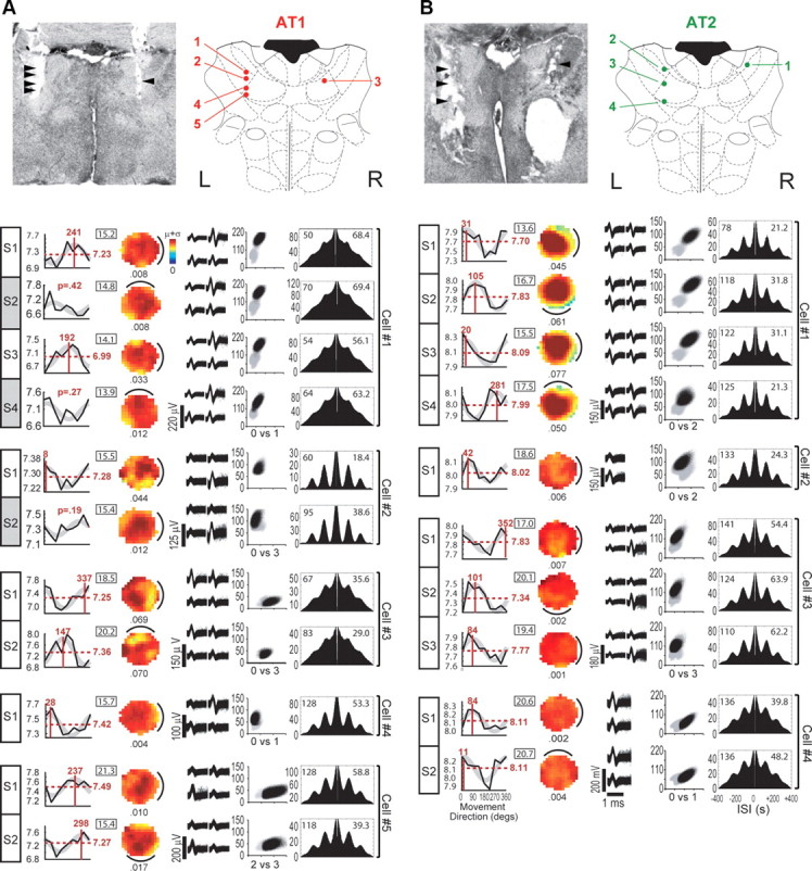
Anterior thalamic theta cells. A, B, Recording sites and session data for anterior thalamic theta cells recorded in rats AT1 (A) and AT2 (B). The top left of each column shows a photomicrograph of electrode tracks with arrowheads indicating recording sites. Top right plots recording sites at −1.3 mm from bregma in rat atlas diagrams adapted from Paxinos and Watson (1997). Each row of graphs shows data from a single recording session, with numbered cells (per rat) indicated by brackets to the right (corresponding to numbers in the atlas diagram above) and session numbers (per cell) indicated by boxed labels (S1, S2, etc.) to the left; white or gray shading of box labels denotes cells that were included or excluded, respectively, from cosine tuning analyses (see Results, Directional modulation of theta cell burst frequencies). From left to right in each row, the first graph plots the DBFT curve (bursting rate in hertz on the y-axis, allocentric movement direction in degrees on the x-axis), with cosine fit shown in gray, red numbers indicating either the preferred burst direction and baseline firing rate (included cells) or the p value for cosine tuning (excluded cells), and black numbers (inside rectangles) denoting the mean running speed, S, for the session. The second graph plots the spatial firing rate map (color scales normalized from 0 to μ+σ, or 1 SD over the mean firing rate in hertz, as shown by the scale bar in the top row of A) with cue position for each session shown by black line and spatial information (bits per spike) shown underneath each map. The third graph shows tetrode spike waveforms, and fourth graph shows cluster plots of peak-to-peak spike amplitude with the cell's spikes shown by black points and all other events shown by gray points (x- and y-axes are identically scaled in millivolts, with tetrode channel numbers displayed below each plot as X vs Y). The fifth graph plots an autocorrelogram for the session, which was obtained by averaging eight directional autocorrelograms (see Fig. 1D) together. Inside the autocorrelogram box, the session duration (in minutes) is given at the top left, and the mean firing rate of theta cell during the session (in hertz) is given at the top right. All anterior thalamic theta cells were recorded in the 80 cm cylinder with a tracking resolution of 4.7 pixels/cm.

DBFT curves.

To analyze how a theta cell's burst frequency was influenced by the rat's running speed in different directions, the eight points of its DBFT curve were subdivided into three movement direction categories: preferred (the three points nearest to θ̄), antipreferred (the three points 180° opposed from θ̄), and orthogonal (the two remaining points, approximating directions ±90° from θ̄). Within each direction category, epochs were subdivided into five speed categories according to the rat's mean running speed s̄ (Eq. 4) during the epoch <10, 10–15, 15–20, 20–25, and 25–30 cm/s. Movement epoch autocorrelograms were then computed independently for epochs within each speed/direction category, and burst frequencies were estimated from the autocorrelograms by the same methods used for obtaining DBFT curves (see above). Estimated burst frequencies were adjusted to a common baseline across cells by subtracting each cell's estimated burst frequency in the 10–15 cm/s speed bin for the orthogonal direction category from all speed bins in all direction categories. Burst frequencies for each speed bin within each direction category were then averaged together across sessions and then cells. Finally, the population-averaged data for each speed bin and direction category were all shifted on the y-axis by a common factor that caused the y-intercept of a linear fit to the all speed data (averaged within speed bins across directional categories) to pass through y = 0, yielding the graph in Figure 5D. Since each autocorrelogram included only a narrow range of running speeds, it was necessary to protect against estimation errors caused by undersampling. To achieve this, three criteria were enforced for inclusion of data from a particular speed bin of a particular cell in the population average: (1) to assure sufficient behavioral sampling, the session had to yield at least 10 s of data (that is, 25 movement epochs of 0.4 s each) for that speed bin; (2) to assure sufficient spike sampling, the mean firing rate of the cell had to be at least 20 Hz when averaged across all of the movement epochs included in that speed bin; (3) to assure that data for each direction category were not drawn from different subpopulations of theta cells in the population average, data for a given speed bin from a given cell had to meet criteria 1 and 2 in that speed bin for all three direction categories to be included in the analysis.

Figure 5.

Population analysis of cosine-tuned theta cells. Cells from rats AT1 and AT2 were recorded in anterior thalamus; for rats MH4–MH6, filled symbols indicate medial septum cells, and open symbols indicate hippocampal cells. A, Circular distribution of preferred movement direction estimates, θ̄, for each theta cell (n = 19) during the first session in which it was recorded with the cue card in the standard position. B, Scatter plot shows estimated base frequency (F̄, x-axis) versus predicted grid spacing (Λ̄, y-axis) for all sessions (n = 31). Dashed lines connect each pair of symbols plotting two different recordings of the same cell, to show within-cell variability of F̄ and Λ̄ across sessions. C, Population averaged DBFT curve (19 theta cells recorded during 31 sessions from 5 rats) is well fit by a cosine function (gray line). D, Population-averaged running speed slopes for movement in the preferred (pref), antipreferred (anti), and orthogonal (ortho) directions of each theta cell (directional ranges indicated by shaded regions in C). Error bars indicate SEM.

Each session's DBFT curve was fit to a cosine function, and fitted parameters were used to analyze modulation of theta rhythm by running speed for different directions (see Results). A significance level for the cosine fit was computed by taking the eight data points on the DBFT curve, resorting them into all possible permutation orders, and repeating the cosine fit for each permutation. The r² value measuring the goodness of fit for each permutation was recorded, and the session's p value for cosine directional tuning was defined as the percentage of permutations that yielded better fits (that is, higher r² values) than the permutation observed in the session's DBFT curve.

Positional and directional firing rate analyses.

Spatial firing rate maps for theta cells were generated by parceling the environment into a lattice of 5 × 5 cm spatial bins and then measuring the amount of time, T_b, the rat spent in each bin, and counting the number of spikes, C_b, fired by the theta cell in each bin. The raw firing rate in each bin was then computed as R_b = C_b/T_b. The spatial information content of the spike train, in bits per spike, was computed from the raw firing rate map by the method of Skaggs et al. (1993). The raw firing rate map was smoothed by a single iteration of adjacent pixel averaging for plots shown in Figures 2–4. For head-direction cells, directional tuning curves were computed using methods described previously (Blair and Sharp, 1995). Like DBFT curves, head-direction cell tuning curves used the convention that degrees increased in the clockwise direction.

Figure 3.

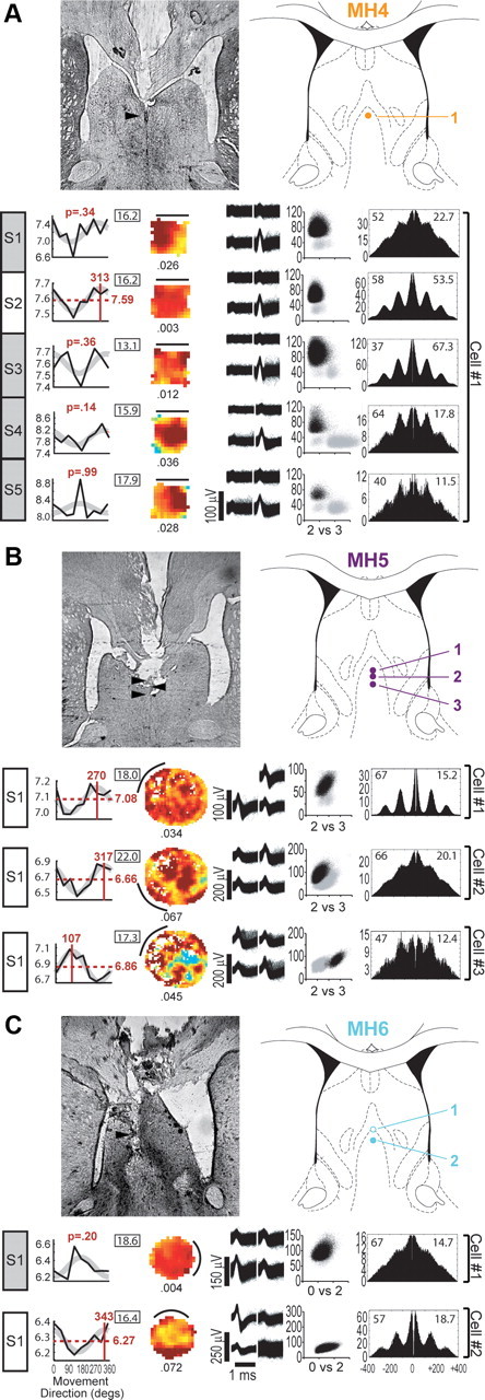
Medial septal theta cells. Histological reconstructions and session data graphs are as described in Figure 2. Atlas diagrams are at +0.5 mm from bregma (open circles indicate sites where a theta cell was recorded but did not meet criteria for inclusion in cosine tuning analyses during any session). A–C, Medial septal theta cells were recorded in the 50 cm square for rat MH4 (A), the 200 cm cylinder for rat MH5 (B), and the 80 cm cylinder for rat MH6 (C). All medial septal recording sessions used a tracking resolution of 1.7 pixels/cm.

Figure 4.

Hippocampal theta cells. Histological reconstructions and session data graphs are as described in Figures 2 and 3. A–C, Hippocampal theta cells were recorded in either the 50 cm square or the 200 cm cylinder for rats MH4 (A) and MH5 (B), and exclusively in the 80 cm cylinder for rat MH6 (C). All hippocampal recording sessions used a tracking resolution of 1.7 pixels/cm.

Data inclusion criteria.

To insure adequate behavioral sampling of each movement direction, the cumulative duration of the sampled movement epochs from a session had to be ≥20 s for each movement direction, otherwise the session was excluded from the study. In addition, single-unit spike data recorded from theta cells had to meet several criteria during each session. First, to insure good single-unit isolation, theta cell spike waveforms were required to show an amplitude of ≥80 μV (peak to peak) against background noise of <30 μV, and interspike intervals had to show a refractory period ≥1 ms. Second, to insure that movement epochs contained enough spikes from which to create autocorrelograms for burst frequency analysis, theta cells were required to maintain a firing rate of >10 Hz throughout the session. Third, to assure that the neuron was a theta cell and not a theta-modulated spatially tuned neuron, theta cells had to exhibit spatial information content of <0.1 bits per spike. Fourth, for each of the eight movement directions, at least 40% of the area under the autocorrelogram's power spectrum between 4–12 Hz had to lie within a 3 Hz band centered on the power spectrum's peak. This insured that the cell's burst frequency was measurable in all movement directions, so that it would be possible to generate a meaningful DBFT curve for the cell.

Numerical methods for simulations.

Theoretical modeling simulations were performed using Matlab and NEURON (Carnevale and Hines, 2006) running on a Windows PC. Detailed descriptions of the numerical methods and source code for simulations are available on the ModelDB website (Hines et al., 2004) under accession number 129067. Briefly, spatially tuned neurons were simulated in NEURON by a single cylindrical compartment with diameter 10 μm and length 10/π μm, with passive membrane resistance and capacitance of R_m = 15 KΩ and C_m = 1.0 μF/cm², and leak reversal potential of E_leak = −65 mV. The simulation time step was dt = 0.1 ms. The model neuron received input from N simulated theta cell spike trains (see Results), with burst frequencies modulated by movement velocity data obtained from a recording session with a real rat. Each input spike triggered a synaptic conductance with dynamics governed by AMPA kinetics from Destexhe et al. (1994). For simplicity, excitatory (AMPA) and inhibitory (GABA_A) conductances were simulated using the same kinetic parameters, except that the synaptic reversal potential was E_AMPA = 0 mV for AMPA and E_GABAA = −80 mV for GABA_A synapses. In simulations with inhibitory input from theta cells, excitatory drive to the model neuron was provided by a voltage-sensitive persistent sodium (Na_P) channel, which was implemented using the kinetic scheme of Uebachs et al. (2010). Active Hodgkin–Huxley kinetics were simulated using the standard NEURON mechanism “hh.mod,” with peak conductance parameters for the delayed rectifier and active sodium channels set to ḡ_K+ = 0.005 mho/cm² and ḡ_Na+ = 0.05 mho/cm², respectively. A vector of spike times generated by the model neuron was accumulated by recording all upward crossings of a threshold at −20 mV, from which path plots and firing rate maps for the simulated spatial neurons were generated.

Results

Experimental results

Single-unit activity was recorded from anterior thalamus, hippocampus, or medial septum while rats (n = 5) foraged freely for food pellets in one of three environments (see Materials and Methods): a small cylinder (80 cm diameter), large cylinder (200 cm diameter), or small square (50 × 50 cm). A subset of neurons were classified as theta cells based on robust 6–8 Hz modulation of their spike trains and high firing rates that lacked spatial tuning (see Materials and Methods). Theta cell spike trains were analyzed to test whether their burst frequencies obeyed a “VCO frequency law,” which predicts that the theta frequency should vary as the cosine of the rat's allocentric movement direction (Burgess et al., 2005, 2007; Giocomo et al., 2007; Hasselmo et al., 2007; Burgess, 2008).

VCO frequency law

As a rat navigates across the floor of a 2D environment, its position x = (x, y) at time t can be derived by calculating the path integral of its velocity, v = dx/dt, from an initial starting location, x(0). Just as the rat's position can be obtained by computing the time integral its velocity, an oscillator's phase, ϕ, can be obtained by computing the time integral of its frequency, ω = dϕ/dt. Consequently, an oscillator with a velocity-dependent frequency will have a position-dependent phase. Oscillatory interference models exploit this principle to propose that path integration is performed by VCOs with instantaneous angular frequencies, (ω₁, ω₂, …,ω_N), that are modulated by v as follows (Burgess et al., 2005, 2007; Giocomo et al., 2007; Hasselmo et al., 2007; Burgess, 2008):

where ϕ_n is the nth VCO's phase in radians, Ω is a shared angular base frequency around which all VCOs are modulated, and d_n is a fixed “preferred vector” in the horizontal floor plane along which the nth VCO frequency is modulated by v. Here, d_n and v are Cartesian vectors in an allocentric coordinate system that is stationary with respect to the lab.

In Equation 11, the dot product term, d_n · v(t), implies that a VCO's frequency should vary as the cosine of the rat's allocentric movement direction (that is, the angle between vectors d_n and v) when running speed (that is, the length of vector v) is held fixed. We investigated whether theta cell burst frequencies were modulated by the rat's movement direction in this predicted manner to test whether theta cells might function as VCOs.

Directional modulation of theta cell burst frequencies

To analyze how theta cell burst frequencies were modulated by the rat's movement direction, the 360° range of directions was subdivided into eight 45° bins, and tracking data from each recording session were parsed to extract time intervals during which the rat was moving continuously in one of these eight directions (Fig. 1A). It was necessary to analyze modulation of theta frequency by movement direction in isolation from modulation by movement speed, so we devised a “speed-balancing” algorithm (see Materials and Methods, Balanced running speed distributions), which made it possible to probabilistically sample movement intervals from the session in such a way that the distribution of running speeds was rendered identical (that is, balanced) in all directions (Fig. 1B, center graph). Theta cell spike trains (Fig. 1C) from movement intervals sampled in this way were analyzed to generate speed-balanced autocorrelograms for each direction (Fig. 1D), and the power spectrum of each autocorrelogram (Fig. 1E) was taken to estimate theta cell burst frequencies in each direction.

Figure 1.

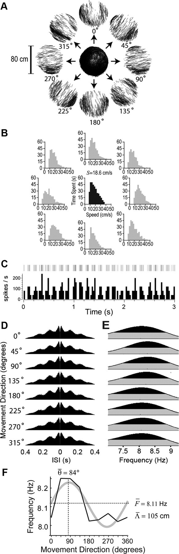
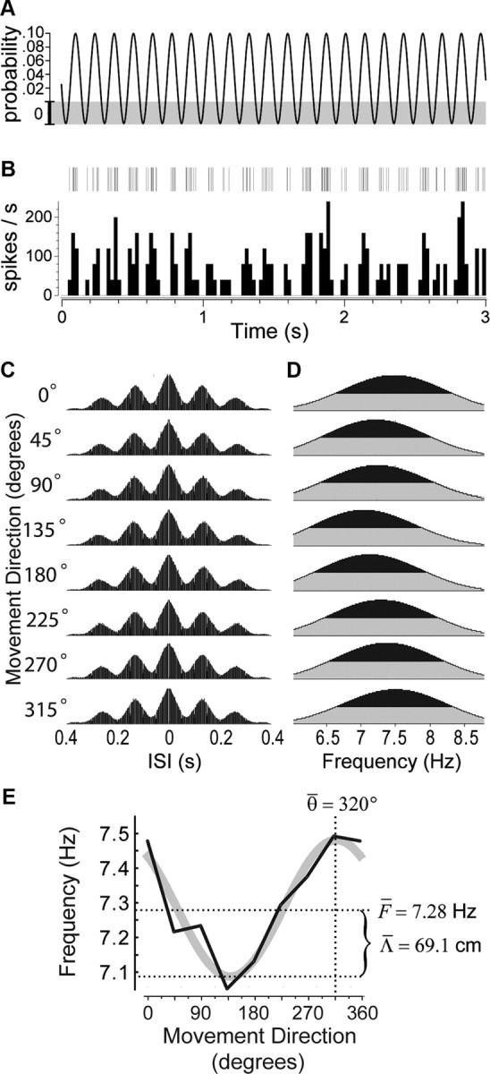
Cosine directional tuning of a theta cell's burst frequency. A, Rat's path during a 136 min recording session in the small cylinder, with cue card at the standard (0°) position; tracking data are decomposed into episodes of movement in eight directions. B, Gray graphs show distributions of running speeds for movements in each direction during the session shown in A; black graph shows the “balanced” running speed distribution derived for the session. C, Short (3 s) segment of the spike raster (top) and rate histogram (bottom, 25 ms bins) for a theta cell recorded in anterior thalamus during the session. D, Spike train autocorrelograms in each movement direction for the theta cell shown in C. E, Power spectra of the autocorrelograms in D. F, DBFT curve (black line) derived from power spectra in E is superimposed on its cosine fit (gray line), with estimates for preferred movement direction (θ̄) and base frequency (F̄) indicated by dashed lines. Predicted grid spacing (Λ̄) is calculated from the amplitude of the fitted cosine function using Equation 16.

A DBFT curve was plotted to depict how a theta cell's burst frequency varied with the rat's movement direction (Fig. 1F). A least-squares gradient search was then performed to fit the eight points of each session's DBFT curve to a cosine function, obtained by rewriting Equation 11 as follows:

where f is the burst frequency in hertz, and θ is the rat's allocentric movement direction. Before fitting, the running speed parameter, S, was set equal to the mean of the balanced running speed distribution. The fitting algorithm returned estimated values for the three parameters decorated by overbars: F̄ is the estimated base frequency (in hertz) around which the theta cell's burst frequency is modulated, and (r̄, θ̄) are polar coordinates estimating length and orientation, respectively, of the VCO's preferred vector, d_n.

The reformulated VCO frequency law of Equation 12 states that the amplitude of the cosine function for directional tuning (that is, the depth of frequency modulation by movement direction) depends on two parameters: r̄ and S. The value of r̄ is assumed to depend on the length of a theta cell's preferred vector, d_n, whereas the value of S depends on the rat's running behavior during the recording session. In our experiments, S ranged between 13 and 22 cm/s (Figs. 2–4), with a mean of 16.9 ± 3.4 cm/s. Within this speed range, oscillatory interference models predict that the cosine function's amplitude, r̄S/2π, should be a few tenths of a hertz at most (see derivation below, in Distribution of predicted grid spacings). Hence, to detect the predicted directional modulation of a theta cell's burst frequency, it was necessary to obtain eight independent measurements of the burst frequency (one for each of the analyzed movement directions), all accurate to within ∼0.1 Hz. To help achieve this required precision of measurement accuracy, sessions were included in the analysis only if they met minimal inclusion criteria for behavioral sampling by the rat and theta rhythmicity of single-unit spike trains (see Materials and Methods, Data inclusion criteria). Sessions that failed to meet these criteria were excluded on the grounds that cosine directional tuning of theta burst frequencies would be undetectable even if it were present, and this limited the number of cells we could analyze.

Inclusion criteria were met by a total of 45 recording sessions obtained from 21 theta cells in five rats (data from all of these sessions are summarized in Figs. 2–4). However, satisfying the minimal inclusion criteria did not guarantee that burst frequency measurements would be accurate enough to detect cosine directional tuning during all sessions in which it might have been present. To test for the presence of cosine directional tuning in each session, Equation 12 was fitted to each session's DBFT curve. A p value was then computed for the cosine fit (see Materials and Methods, DBFT curves), providing a confidence measure for the presence of cosine tuning, as well as for the accuracy of the fitted cosine tuning parameters. The degree of overlap between a session's DBFT curve and the fitted cosine function was inversely proportional to the p value computed for the fit. A significance level of p < 0.05 (the standard cutoff for two-tailed tests) was beaten by 14 of 45 (31%) of the recording sessions, a much greater proportion than would be expected under the null hypothesis that theta cell burst frequencies were not directionally modulated (binomial test, p < 0.0001). A less stringent significance level of p < 0.1 (the standard cutoff for one-tailed tests) was beaten by 31 of 45 (69%) of the recording sessions, which again was a much greater proportion than chance would predict (binomial test, p < 0.0001). These results indicate that among recording sessions that met criterion for inclusion in the analysis, cosine-like directional tuning was much more prevalent than would be expected by chance alone.

Having thus established the presence of directional tuning, we sought to characterize this tuning by further analyzing the data from those sessions in which a robust directional tuning signal was observed. For a session to be included in these analyses, its DBFT curve was required to exhibit a cosine fit of p < 0.1 or better. This criterion was met by at least one session for 19 of 21 (90%) of the recorded theta cells (9 of 9 cells in anterior thalamus, 5 of 6 cells in medial septum, and 5 of 6 cells in hippocampus). Whenever possible, a single theta cell was recorded repeatedly across multiple sessions. In some cases, a cell's DBFT curve beat the p < 0.1 criterion during some sessions while failing to beat criterion during other sessions. In many (but not all) of these cases, the DBFT curve resembled a cosine function even during excluded sessions that failed to beat the p < 0.1 criterion, and tuning parameters were similar to those observed for included sessions (Fig. 2A, cell 1). Such variability in the quality of the cosine fit from different sessions with the same cell may have been caused by variation of uncontrolled factors (such as the rat's movement behavior and the quality of single-unit isolation) that affected the accuracy of theta cell burst frequency estimates from one session to the next.

The proportion of sessions passing the p < 0.1 reliability criterion for cosine tuning differed among the three targeted brain structures. The criterion was beaten by 18 of 21 (86%) of the sessions from anterior thalamus (Fig. 2), 5 of 10 (50%) of the sessions from medial septum (Fig. 3), and 8 of 14 (57%) of the sessions from hippocampus (Fig. 4). This variation in the reliability of cosine tuning across brain structures does not necessarily indicate that the prevalence of cosine tuning differed among structures, because recordings obtained from different structures also varied in their video tracking resolution, session duration, and geometry of the recording environment (Figs. 2–4; also see Materials and Methods), all of which are factors that can influence the accuracy of burst frequency estimates. Hence, variability in the experimental conditions may have affected the proportion of sessions beating the cosine tuning threshold, making it difficult to compare the prevalence of cosine tuning across different brain structures.

Figure 5C shows a population DBFT curve which was generated by averaging curves from all session beating the p < 0.1 threshold, first over sessions (n = 31) and then over cells (n = 19). Before averaging, individual DBFT curves were aligned with respect to their cosine tuning parameters (θ̄ on the x-axis, F̄ on the y-axis). The resulting population curve was well fit by Equation 12 (p < 0.0025), supporting the conclusion that some theta cells exhibited cosine-like directional tuning of their burst frequencies, in accordance with the VCO frequency law.

Cue control over preferred movement directions

Firing rate maps of spatially tuned neurons can follow rotations of familiar landmark cues (Muller and Kubie, 1987; Taube et al., 1990; Knierim et al., 1995, 1998; Hafting et al., 2005; Solstad et al., 2008). If spatial neurons derive their positional tuning from theta cells with directionally tuned burst frequencies, then DBFT curves of theta cells should exhibit a similar tendency to rotate with landmarks. To test this, we recorded theta cells across multiple sessions whenever possible, and sometimes rotated a landmark cue on the wall between sessions (the extramaze light source and experimenter's entry position were also rotated along with the cue card; see Materials and Methods). DBFT rotation errors (henceforth denoted by ε_DBFT) were quantified as the difference between rotation of θ̄ and the cue rotation angle. For 12 pairs of consecutive sessions across which a theta cell was held (Table 1), the circular mean of ε_DBFT was −9.1 ± 13.4° (Fig. 6A). Circular statistics indicated that ε_DBFT values were nonuniformly distributed (Rayleigh's Z = 7.28, p = 0.0002) and significantly clustered near zero (V = 0.77, p = 0.00002), supporting the conclusion that DBFT curves were often controlled by landmark cues.

Table 1.

Directional tuning and rotation errors across pairs of repeated sessions

Cell ID	Session	θDBFT	θHD	ΔθDBFT	ΔθHD	ΔθCUE	ϵDBFT	ϵHD	ϵINT
AT1 cell 1	S1	241	241
	S3	192	253	−49	12	0	−49	12	61
AT1 cell 3	S1	337	311
	S2	147	112	−190	−199	−90	−100	−109	−9
AT1 cell 5	S1	237	×
	S2	298	×	61		90	−29
AT2 cell 1	S1	31	210
	S2	106	286	75	76	90	−15	−14	1
	S3	20	202	−86	−84	−90	4	6	2
	S4	281	107	−81	−95	−90	9	−5	−14
AT2 cell 3	S1	352	237
	S2	101	347	109	110	90	19	20	1
	S3	84	33	−17	46	−90	73	136	63
AT2 cell 4	S1	84	176
	S2	11	97	−73	−79	−90	17	11	−6
MH5 cell 1	S1	278	×
	S2	263	×	−15		0	−15
	S3	129	×	−134		−90	−44
	S5	139	×	10		0	10
Circular mean							−9.1	+3.2	+10.9
SD							13.4	22.1	12.7
Unsigned mean							32.0	39.1	19.6
SD							8.9	19.7	10.0

Each row corresponds to an experimental session, with animal, cell, and session numbers listed under Cell ID and Session. All numeric values are in degrees. The preferred movement directions of theta cells are listed under θ_DBFT, and the preferred firing directions of simultaneously recorded head direction cells are listed under θ_HD (× denotes session during which no head direction cell was recorded). Rotations of the DBFT curve, head direction cell tuning curve, and cue card (in comparison with the session from the row above) are listed under Δθ_DBFT, Δθ_HD, and Δθ_CUE, respectively. DBFT, head direction, and internal rotation errors are listed under ϵ_DBFT, ϵ_HD, and ϵ_INT, respectively, where ϵ_DBFT = Δθ_DBFT − Δθ_CUE, ϵ_HD = Δθ_HD − Δθ_CUE, and ϵ_INT = ϵ_HD − ϵ_DBFT.

Figure 6.

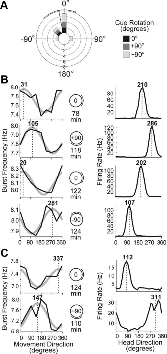
Cue control of DBFT curves. A, Circular histogram plots distribution of DBFT rotation errors with respect to the cue card for 12 pairs of consecutive sessions over which a theta cell was held (Table 1); shading indicates angle of cue rotation between sessions, and black lines show the mean and SD of rotation error. B, Left column shows DBFT curves for an anterior thalamic theta cell (rat AT2, cell 1 from Fig. 2B); right column shows tuning curves for a head-direction cell recorded simultaneously in the 80 cm cylinder across four consecutive cue rotation sessions. Both cells rotated their directional tuning functions along with the position of the cue (indicated by diagrams). C, A pair of sessions during which a theta cell (rat AT1, cell 3 from Fig. 2A) and simultaneously recorded head-direction cell failed to follow rotations of the cue but maintained coupling of their directional tuning relative to one another.

DBFT curves did not always follow landmark cues, since ε_DBFT was large for some session pairs. To further study these cases, we exploited the fact that theta cells in anterior thalamus were sometimes recorded simultaneously with neighboring head-direction cells. In these cases, it was possible to measure a head-direction error (ε_HD) that compared rotation of the cue with rotation of the head-direction cell tuning curve (Table 1). For eight pairs of consecutive sessions across which both theta and head-direction cells were held, the circular mean of ε_HD was 3.2 ± 22.1°, and ε_HD values were clustered near zero (Rayleigh's Z = 6.2, p = 0.0004; V = 0.86; p = 0.00005). These results indicate that head-direction cell tuning curves were controlled by the landmark cue in a manner similar to DBFT curves. In cases where DBFT curves closely followed the cue, head-direction cell tuning also tended to follow the cue (Fig. 6B), but in cases where DBFT curves were poorly controlled by the cue, head-direction cell tuning also tended to be poorly controlled by the cue (Fig. 6C).

To analyze coupling between the directional tuning of theta and head-direction cells, an internal rotation error (ε_INT) was computed to compare rotation of theta cell DBFTs against rotation of head-direction cell tuning curves (Table 1). The circular mean of ε_INT was 10.9 ± 12.7°, and ε_INT values were clustered near zero (Rayleigh's Z = 2.8, p = 0.056; V = 0.591; p = 0.008), indicating that DBFT curves and head-direction cell tuning curves tended to rotate in tandem by similar amounts. Further supporting this, the absolute (that is, unsigned) means of ε_HD and ε_DBFT (Table 1, bottom) did not differ significantly from one another (Mann–Whitney U = 40, p = 0.92), but the unsigned mean of ε_INT was significantly smaller than that for ε_DBFT (Mann–Whitney U = 62.5, p = 0.03), implying that DBFT curves were more tightly coupled to head-direction cells than to the landmark cue; that is, theta cell DBFT curves and head-direction cell tuning curves both showed a significant tendency to follow rotations of the landmark cue (as indicated by circular statistics on each population). But both also showed incidences of failure to follow the cue, and in these instances, the directional tuning functions of theta and head-direction cells were better coupled to one another than to the landmark. A likely interpretation of these results is that rotation of the cue sometimes failed to “fool” the rat into rotating its directional reference frame with the cue, but in these cases, preferred movement directions of theta cells remained anchored to the rat's internal directional reference frame (as indicated by better coupling of theta cells to head-direction cells than the cue).

To synthesize spatial tuning functions in two dimensions, different theta cells would need to integrate the rat's movement velocity along vectors with different orientations (see below, Spatially tuned neurons in an open field). To test this prediction, a circular distribution of θ̄ values was plotted for one recording session from each theta cell (Fig. 5A). To maintain the same directional reference frame for all data points, the distribution included only one session from each cell, chosen at random from all sessions during which the cell was recorded with the cue card and extramaze light source in a “standard” position. Three cells were not recorded during a session with cues in the standard position, so for these cells, a nonstandard cue session was randomly chosen, and the cue rotation angle (−90° or +90° from standard) for the chosen session was subtracted from θ̄ before it was entered into the distribution. Values of θ̄ were uniformly distributed (Rayleigh's Z = 2.027, p = 0.13; Rao's spacing test U = 126.0, p > 0.5), supporting the conclusion that each theta cell was tuned to have its own preferred movement direction.

Amplitude of directional modulation

The fitted value of r̄ estimated the amplitude of directional frequency modulation around F̄, for the case where running speed was equal to S. If theta cells function as VCOs, then r̄ estimates the length of the VCO's preferred movement vector. Empirical values of r̄ can be tested against theoretical predictions by recognizing that when a grid cell is formed by interference among VCOs, the vertex spacing of the grid is inversely proportional to VCO vector length (Burgess et al., 2007; Giocomo et al., 2007; Hasselmo et al., 2007). For the case of an equilateral grid, the smallest obtainable vertex spacing is formed by combining three VCOs with preferred movement vectors of the same length, r̄ = |d₁| = |d₂| = |d₃|, and differing orientations that are 120° apart from each other. To compute the spacing of a grid cell formed from such a triplet of VCOs, we may express the phases of the three oscillators (k = 1, 2, 3) as follows:

where Φ is a common “reference phase” shared among all VCOs (Eq. 17). By the VCO envelope formula (Eq. 20), we obtain the following:

where the three vectors given by D₁ = d₁ − d₂, D₂ = d₂ − d₃, and D₃ = d₃ − d₁ have identical length D = |D₁| = |D₂| = |D₃|, and their directions are also 120° apart. Thus, the envelope can be regarded as a sum of three straight cosine gratings with the spacing λ = 2π/D. The spacing Λ̄ of the hexagonal grid formed by these three cosine gratings is as follows:

Based on the geometry, we have D = $\sqrt{3}$r̄, which leads to the following formula for the predicted grid spacing:

Solving Equation 16 with empirically measured values of r̄, we may estimate the smallest vertex spacing obtainable for grid cells formed by phase interference among theta cells similar to those we recorded. Figure 5B (y-axis) shows that the predicted minimal grid spacings were distributed over a range of 25–225 cm (Fig. 5B, y-axis), which is similar to the range of vertex spacings that has been reported for grid cells in dorsal medial entorhinal cortex (Hafting et al., 2005; Sargolini et al., 2006; Brun et al., 2008b). Plugging this range of predicted grid spacings into Equation 16 and then algebraically solving for r̄, we can then use Equation 12 to estimate the range over which r̄ should vary at the mean balanced running speed of S = 16.9 cm/s. This calculation yields a prediction that the cosine amplitude coefficients of DBFT curves should range between about 0.05 and 0.45 Hz, emphasizing the point made above (see Directional modulation of theta cell burst frequencies) that the predicted directional modulation of theta frequencies is quite small.

It should be emphasized once again that these calculations assume grids are formed from triplets of theta cells with preferred direction vectors that are 120° apart. But there are many different ways to form a hexagonal grid from interference among VCOs (Burgess, 2008), and the slope of the inverse relationship between vector length and vertex spacing depends on exactly how VCOs are combined form the grid. For example, adding six VCOs with preferred directions that are 60° apart would lead to a predicted grid spacing that is larger than that in Equation 16 by a factor of $\sqrt{3}$, and an adjusted range of grid spacings of 43–390 cm, which would still be within the range of empirically observed values (Hafting et al., 2005; Sargolini et al., 2006; Brun et al., 2008b).

Modulation of burst frequencies by running speed

The fitted value of F̄ estimated the base frequency around which theta cell bursting was modulated. Values of F̄ showed variability among different rats across an approximate range of 6–8 Hz, and showed a lesser degree of variability (up to ∼1 Hz) across different sessions within the same rat (Fig. 4B, x-axis). This pattern of results is consistent with prior studies showing variability of theta frequency across rats and sessions (Jeewajee et al., 2008b). If the base frequency remains rigidly constant at all times and does not vary with running speed, then Equation 11 dictates that a VCO's frequency should increase with running speed when the rat moves in the VCO's preferred direction, and decrease with running speed when the rat moves in the opposite (antipreferred) direction. Averaged across all directions, these opposing influences should cancel each other out, yielding a prediction that the mean VCO frequency would be identical for all running speeds. Contradicting this prediction, prior studies have shown that the theta frequency increases with running speed when movement direction is disregarded (Rivas et al., 1996; Geisler et al., 2007; Jeewajee et al., 2008a). One simple way to account for these results is to assume that the VCO base frequency [Eq. 11, Ω(t)] increases in proportion with running speed (Burgess, 2008). As long as this speed-dependent base frequency remains identical for all VCOs, then path integration would not be impaired.

To investigate modulation of the base frequency by running speed, an analysis was conducted in which theta cell burst frequencies were analyzed as a function of the rat's running speed in directions parallel, antiparallel, and orthogonal to each cell's preferred movement direction (Fig. 5D). Averaging results across sessions and then cells, it was found that theta cell burst frequencies increased with running speed in all directions, and the slope of speed modulation was steepest for the preferred and shallowest for the antipreferred direction. The observation that the theta frequency increased with running speed in all directions (rather than increasing in the preferred and decreasing in the antipreferred direction) suggests that the base frequency was not constant, but instead increased with running speed. As long as Ω(t) varies only with running speed, and not with movement direction, then the VCO frequency law still dictates that theta burst frequencies should vary as the cosine of the rat's movement direction, as we have observed.

Analytic simulations of spatially tuned neurons

Experimental results presented above suggest that VCO signals may be encoded by spike trains of rhythmically bursting theta cells. Computer simulations were performed to test whether spatially tuned neurons could be formed by phase interference among theta cells with firing properties similar to those observed in our experiments (source code and input data for simulations are available on ModelDB). Before describing these simulation results, we first introduce an analytic expression for the spatial envelope function that is synthesized from phase interference among any arbitrary set of VCOs.

VCO envelope and carrier equations

Equation 11 dictates that the nth VCO's frequency varies linearly with the rat's velocity along a preferred vector, d_n, so that a component of the VCO's phase becomes dependent on the rat's position along that same vector. To isolate this position-dependent phase component, we may separately integrate the two summed terms in Equation 11, and thereby express the instantaneous phase of the VCO as a sum of two terms:

where Φ is a common “reference phase” shared among all VCOs [obtained by integrating the base frequency, Ω, between times 0 and t from an initial starting phase, Φ(0)], and δ_n is the nth VCO's unique offset from the reference phase, which depends upon the rat's spatial position, x(t), as follows:

with δ_n(x(0)) = ϕ_n(0) − Ω(0) denoting the nth VCO's initial offset from the reference phase. It follows from Equation 18 that if a rat navigates to an arbitrary position, x(t), then the nth VCO's phase at that position will be offset from the reference phase by an amount that depends strictly upon the distance of x(t) from the rat's starting position, x(0), along the VCO's preferred vector, d_n. Moreover, if all VCOs share the same reference phase, then their phase offsets from each other will also depend strictly on the rat's location. Consequently, every location in space will be encoded by a specific pattern of phase relationships among VCOs. If VCO phase relationships depend strictly on the rat's position, then phase interference among VCOs is guaranteed to synthesize an envelope function that “sits still” in space, regardless of the rat's movement trajectory through the environment (Burgess et al., 2005; 2007). The outputs from N VCOs may be thus summed together to generate an interference pattern as follows (Fig. 7A):

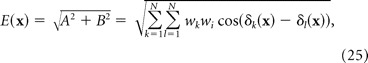
where w_n is a weighting coefficient for the nth VCO. The second step in Equation 19 states that the sum of VCO outputs can be rewritten as a product of just two terms: a carrier signal C(t) that varies over time, and an envelope signal E(x) that varies over space. By exploiting a trick based on Euler's formula l (Hartmann, 1998), E(x) can be expressed as a sum of complex exponential terms by the following VCO envelope equation:

where i = $\sqrt{1-}$ inside the exponential function. The VCO envelope defined by Equation 20 behaves much like the firing rate of a spatially tuned neuron, growing large at locations where many VCOs are synchronized (constructively interfering) and becoming small at locations where most VCOs are desynchronized (destructively interfering).

Figure 7.

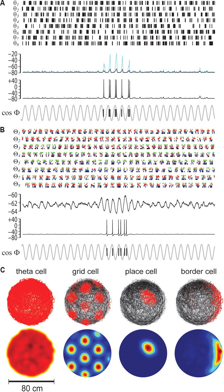
Analytic simulations of spatial neurons formed from theta cells. A, Simulated rat runs at 25 cm/s along a 1.0 m linear track, while eight theta VCOs (θ₁–θ₈) oscillate at differing frequencies; all VCO phases are perfectly aligned in the center of the track (dashed vertical line). Summing VCO outputs can produce interference patterns that mimic the spatial firing patterns of grid or place cells (see Results, Place cell synthesized from theta cells on a linear track). B, Activity bump (shaded circles) circulates around a ring oscillator circuit to generate theta rhythm at a frequency that varies with the rat's velocity along a preferred vector, d_n. C, A matrix of ring oscillator circuits contains a distributed population of theta cells from which different kinds of spatially tuned neurons can be formed (see main text); simulated tuning functions (Model) are shown beside real fining rate maps (Data) for a hippocampal place cell (reprinted from Leutgeb et al., 2007), grid cells in dorsal and ventral entorhinal cortex (reprinted from Hafting et al., 2005), and a border cell in entorhinal cortex (reprinted from Solstad et al., 2008).

Equation 19 states that the spatial envelope signal is multiplicatively modulated by a temporal carrier signal, assumed here (as in prior oscillatory interference models) to account for theta modulation of spatial neuron spike trains. The carrier signal can be written as follows:

where

with

and

Analytic model of spatial neurons formed from theta cells

The VCO envelope equation implies that any neuron which can detect synchrony among VCOs (by firing selectively when their phases converge) is guaranteed to “pick out” a selected spatial region of the rat's environment (by firing only when the rat is located within that region). Prior interference models have demonstrated this for the special case of grid cells, showing how phase interference among VCOs can synthesize envelopes that form a hexagonal lattice tiling the environment (Burgess et al., 2005, 2007; Giocomo et al., 2007; Hasselmo et al., 2007; Burgess, 2008; Zilli and Hasselmo, 2010). Here, we expand on these results by showing that, more generally, the VCO envelope can mimic almost any spatial function and thereby simulate the firing rate maps of almost any spatially tuned neuron (including place and border cells, in addition to grid cells).

A simplified case is illustrated in Figure 7A, which plots output from eight VCOs (modeled as cosine functions) while a simulated rat runs at a constant speed of 25 cm/s along the length of a 1 m linear track. In this example, all of the VCOs have different fixed frequencies, and they converge in phase at the center of the track. If a postsynaptic neuron sums input from just two of these eight VCOs, then its output can generate a beat envelope that waxes and wanes at fixed intervals along the length of the track, mimicking the spatially periodic firing pattern of a grid cell as in prior models (Fig. 7A, E_grid). But if the target neuron sums input from all eight of the VCOs, then its output will grow large only at the center of the track where all VCO phases converge, mimicking the unitary firing field of a place cell (Fig. 7A, E_place). Thus, detection of phase convergence among few VCOs (a common event that recurs at fixed intervals along the track) simulates a grid cell, whereas detection of phase convergence among many VCOs (a rare event which occurs at just one location on the track) simulates a place cell.

More generally, a postsynaptic neuron can generate almost any spatial function by detecting phase convergence among a properly chosen set of VCOs. To see why this is so, it is helpful to rewrite Equation 20 in the following form:

where A and B are given by Equations 23 and 24, and x is now assumed to be a vector representing the rat's location in a 2D environment instead of a linear track (note that generalization to arbitrary dimensions is possible; see Discussion). Here, the envelope equation becomes a sum of 2D cosine functions (or gratings) formed by interferences between all possible pairs of the N VCOs, indexed by k and l. These cosine gratings define the components of the envelope's 2D spatial frequency spectrum, and they are fully determined by the preferred vectors (d₁, d₂, …, d_N), weighting coefficients (w₁, w₂, …, w_N), and starting phases [ϕ₁(0), ϕ₂(0), …, ϕ_N(0)] of the VCOs that interfere with one another to synthesize the envelope. If these parameters are properly chosen, then a sufficiently large number of VCOs should be able to approximate the spatial frequency spectrum of almost any desired spatial function.

Let us suppose that the rat brain contains a large and diverse population of VCOs, all sharing a common reference phase as assumed by Equations 17 through 25, and that each VCO signal is generated by a rhythmically bursting theta cell (as suggested by our experimental findings above). Such a population of theta cells can encode a basis set from which arbitrary spatial tuning functions could be synthesized. A different spatial envelope would be formed by interference among any unique subset of theta cells in the population, and a few key parameters would determine the frequency spectra (and thus the shapes) of these envelope functions. As noted above, one such parameter is the temporal phase of each VCO signal. Hence, to generate a diversity of different spatially tuned neurons, it would be useful for VCOs to be implemented as multiphase oscillators, which generate multiple copies of the same VCO signal at diverse phase shifts. Supporting this possibility, there appears to be a continuous gradient of theta phase along the septotemporal axis of the hippocampus (Lubenov and Siapas, 2009).

This phase diversity requirement entices us to conceptualize the CPG circuit for theta rhythm as “ring oscillator” composed from a circular layer of theta cells (Blair et al., 2008). A localized “bump” of activity can circulate around the ring at the theta frequency, so that each cell in the ring generates rhythmic theta bursts on a different phase of the same VCO cycle (Fig. 7B). To regulate the VCO frequency in accordance with Equation 11, the ring may receive an external driving input that encodes the rat's translational velocity along the ring's preferred vector, d_n. In a population of ring oscillators with different velocity inputs, the nth ring oscillator serves as a multiphase VCO that performs translational path integration along its own preferred vector, d_n. This ring oscillator model of translational path integration is quite similar to hypothetical ring attractor models of angular path integration by head-direction cells (Skaggs et al., 1995; Redish et al., 1996; Zhang, 1996; Song and Wang, 2005), raising the possibility that translational and angular path integration might both be performed by similar ring attractor circuits (Blair et al., 2008; Mhatre et al., 2010).

Figure 7C illustrates a hypothetical arrangement of ring oscillators within a structured matrix of VCOs that contains a distributed population of theta cells from which many different spatial tuning functions can be synthesized. The VCO parameters of each theta cell in Figure 7C are determined by the cell's position in the matrix; theta cells residing in the same ring share the same preferred vector, and thus generate the same VCO signal at different phase shifts. Theta cells residing in different rings have different preferred vectors, and thus generate different VCO frequencies. The matrix is organized so that rings in the same row are modulated by running speed with the same slope (and thus have VCO vectors of identical length), whereas rings in the same column prefer movement in the same direction (and thus have VCO vectors of identical orientation).

A target neuron that sums input from theta cells in the VCO matrix can simulate the positional firing properties of almost any spatially tuned neuron, depending on the rows, columns, and ring positions of the theta cells that provide its input. This is illustrated on the right side of Fig. 7C, which shows analytic envelope functions that were simulated by solving Equation 20. To simplify the derivation of spatial envelopes in these simulations, the rat's initial starting position, x(0), was set equal the origin of the spatial coordinate system, which corresponded to the center of the arena. In addition, the starting phases, ϕ_n(0), for all VCOs were initialized to zero, and all VCO weighting coefficients, w_n, were set uniformly equal to 1. Spatial tuning functions were simulated by assigning preferred vectors, [d₁, d₂, …, d_N], to a set of N VCOs and then solving Equation 20 at each point on a square lattice representing positions in a 1 m² square environment. The amplitude of E(x) was converted to a “firing rate” by filtering through a spike threshold:

where R(x) is the firing rate at x, H is the Heaviside function, and κ represents the spike threshold which was set to κ = 0.7 × max[E(x)] for all simulations presented here.

As in prior oscillatory interference models (Burgess et al., 2005, 2007; Giocomo et al., 2007; Hasselmo et al., 2007; Burgess, 2008), a target neuron that receives input from properly chosen theta cells can simulate a grid cell with various vertex spacings (blue and green lines in Fig. 7C). Here, the vertex spacing depends on which matrix row theta cells reside in, and the grid orientation depends on which columns theta cells reside in. But in addition to grid cells, other types of spatially tuned neurons can also be formed. For example, suppose that a target neuron's input comes from theta cells residing in different rows of the same column (Fig. 7C, red lines). Since all of these theta cells have preferred vectors of the same orientation (but with different slopes of speed modulation), the target neuron fires along a linear band oriented perpendicular to the preferred vector orientation. This linear band can mimic the firing rate map of a border cell that fires along a straight wall (Fig. 7C, bottom right) or of a boundary vector cell (Lever et al., 2009) that fires at a fixed distance from the wall (data not shown). Alternatively, if the target neuron's input comes from theta cells in every column of a single row, then it can simulate a place cell (Fig. 7C, top right). Like the vertex spacing of a grid cell, the size of a place cell's firing field would depend on which row of the matrix provides input to the target neuron.

As a general rule, a target neuron that receives input from many theta cells will tend to fire in very few (and possibly zero) subregions within a the circumscribed area of any given environment (since phase convergence among many theta cells is a rare event that occurs at very few locations); the shape and size of this subregion will depend on exactly which theta cells provide the neuron's input. Conversely, a target neuron that receives input from just a few theta cells will tend to fire within multiple subregions of an environment (since phase convergence among a small number of theta cells is a common event that recurs at multiple locations). For example, we have already seen that grid cell firing patterns can emerge from interference among a few systematically chosen theta cells. Alternatively, interference among randomly chosen theta cells can mimic the firing patterns of neurons that fire at multiple locations that are randomly distributed (results not shown), such as those found in the dentate gyrus (Leutgeb et al., 2007).

Biophysical simulations of spatially tuned neurons

In Figure 7, spatial neurons were simulated by analytically solving Equation 20 to generate envelope functions. Hence, the envelopes were obtained by linearly summing a basis set of idealized VCOs, each represented as a velocity-modulated cosine function consisting of a single fundamental harmonic component. But our experimental data suggest that VCO signals may be encoded by noisy theta cell spike trains. Unlike idealized cosine VCOs, these noisy spike trains contain many complex harmonics in addition to the “fundamental” theta frequency of their bursting rate. There is thus no guarantee that spike trains from biological theta cells could interfere with one another to synthesize spatial envelopes, because the additional harmonics introduced into the VCO signals by noise and the spiking process—which are not accounted for by the VCO envelope equations—might interfere with one another in ways that compromise the spatial rigidity and trajectory invariance of the envelopes. Moreover, a biological neuron typically does not compute a perfect linear sum of its inputs, as assumed in the analytic simulations of Figure 7.

Simulating theta cell spike trains

To investigate whether spatially tuned neurons can be formed from spiking theta cells similar to those we observed in our experiments, we simulated theta cell spike trains using a Poisson process. A theta cell spike was generated pseudorandomly at each simulation time step (dt = 2 ms) with an oscillating probability that varied with the amplitude of an ideal cosine VCO (Fig. 8A). Experiments indicated that the base frequency of theta cell VCOs increased with running speed (Fig. 5D). To incorporate this result into simulations of theta cell spike trains, the following version of the VCO frequency law was used:

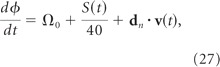where dϕ/dt is the instantaneous angular frequency of the oscillating spike probability, S(t) is the rat's instantaneous running speed, and Ω₀ + S(t)/40 defines the speed-dependent base frequency, so that Ω(t) increases with running speed at a slope of 1/40 Hz/cm/s. To generate simulated spike trains, movement velocity data from a 60 min segment of an experimental recording session were upsampled to 500 Hz (from the video tracking rate of 30 Hz) to match the simulation time resolution of dt = 2 ms. At each time step, the VCO phase, ϕ(t), was computed by numerically integrating the VCO frequency defined by Equation 27 across the 60 min session, with the values for movement velocity derived from the tracking data. Spike probability at each time step was then computed as follows:

where H is the Heaviside function. Thresholding by H gives a spike probability of P(t) = 0 in an interval of width π/2 centered upon the valley of each theta cycle (so that the simulated theta cell falls silent between bursts on each cycle). Outside of this silent interval, P(t) varies as a continuous function of the VCO amplitude, reaching a maximum value of 0.5 spikes per dt at the peak of each theta cycle. When Ω₀ was set to 7 Hz (as in simulations presented here), Equation 28 produced simulated theta cell spike trains with a mean spiking rate of ∼100 Hz (note that a refractory period of 2 ms between spikes was automatically conferred by the 2 ms time resolution of the simulations). To obtain firing rates lower than 100 Hz, spikes were randomly selected for deletion from the train with a probability inversely proportional to the desired firing rate. When simulated spike trains were analyzed using the same algorithms that were used for experimental data analysis, simulated theta cells exhibited directional tuning of their burst frequencies similar to that observed for real theta cells (Fig. 8).

Figure 8.

Simulated theta cell spike train. A, Velocity data were used to modulate the frequency of a cosine VCO, which was then converted into a probability (y-axis) of spike occurrence at each simulation time step (x-axis; bin size, 2 ms); the shaded area is below spiking threshold. B, A short (3 s) segment of the spike raster plot for a simulated theta cell is shown above its corresponding rate histogram (25 ms bins). C, Velocity data from an experimental session (60 min) were used to modulate the simulated theta cell's burst frequency, and the resulting spike train was analyzed with the same software used for neurophysiological data analysis, yielding spike train autocorrelograms for each movement direction. D, Power spectra of the autocorrelograms in C. E, DBFT curve derived from power spectra in D, along with VCO parameter estimates (θ̄, Λ̄, F̄) derived from the curve. The actual VCO parameters used in this simulation were θ = 315°, Λ = 60 cm, and F(t) = 7.0 + 0.25 r(t) Hz (the base frequency was linearly dependent on running speed, to approximate experimental results shown in Fig. 5D). It can be seen that the data analysis algorithm recovered these VCO parameters with good accuracy.

Place cell synthesized from theta cells on a linear track

Based on existing knowledge of hippocampal and thalamocortical circuits, it is reasonable to assume that many of the theta cells we recorded in medial septum (Fig. 3) and hippocampus (Fig. 4) were inhibitory neurons (Ranck, 1973; Freund and Antal, 1988), whereas theta cells in the anterior thalamus (Fig. 2) may have been excitatory thalamocortical projection neurons (Jones, 1985; Tsanov et al., 2011b). We thus conducted simulations to test whether spatial tuning functions could be formed by inhibitory versus excitatory inputs to a postsynaptic target neuron from theta cells.

To compare interference among excitatory versus inhibitory theta cells, we replicated the place cell simulation of Figure 7A, in which a rat runs at constant speed across a linear track. Each of the eight cosine VCO signals in Figure 7A was converted into a theta cell spike train by the method illustrated in Figure 8. The NEURON simulation environment (Carnevale and Hines, 2006) was then used to create a single-compartment model of a postsynaptic target cell, which received identically weighted inputs (either excitatory or inhibitory) from the eight simulated theta cell spike trains.

In simulations where theta cell spike trains triggered IPSPs, the target neuron was able to fire selectively in the center of the track by detecting location-dependent synchrony among its inputs from theta cells (Fig. 9A). It may seem counterintuitive that synchronization among inhibitory inputs would excite the postsynaptic neuron, but similar results were also reported by Zilli and Hasselmo (2010) in simulations of grid cells. This paradoxical excitation of the postsynaptic cell by synchronized inhibitory inputs occurs because desynchronized input from inhibitory theta cells produces a constant, uninterrupted barrage of inhibition that prevents the target neuron from firing; when inhibitory theta bursts become synchronized, prolonged relief from inhibition (lasting tens of milliseconds) occurs during gaps between synchronized theta bursts. Under the influence of an excitatory drive, which was provided in our simulations by a persistent sodium (Na_P) current (Fig. 9A, blue trace), the target neuron can fire reliably during the disinhibitory gaps. Hence, by detecting coincident gaps between synchronized theta bursts, the target neuron can measure location-dependent burst synchrony among its inputs from inhibitory theta cells, so that its firing rate approximates the spatial envelope defined by Equations 20 and 25.

Figure 9.

Biophysical simulations of spatially tuned neurons formed from theta cells. A, Simulated rat runs at 25 cm/s along a linear track; a postsynaptic neuron receives inhibitory input from eight theta cells, modeled as Poisson spike trains generated from cosine VCO functions (θ₁–θ₈) shown in Figure 7A. The top trace shows membrane voltage (V_m) for simulations with a purely passive membrane (black) or with Na_P current but no spike channels (blue); the bottom V_m trace shows simulations with both Na_P and spike channels. At the bottom, the raster plot shows phase precession of spikes with respect to the VCO reference phase, Φ (Eq. 17). B, Same as A except that the target neuron now receives excitatory input from 32 theta cells, divided into eight groups (Θ₁–Θ₈) that each consist of four Poisson spike trains (shown in different colors) that were independently generated from VCO functions (θ₁–θ₈) in Figure 7A. The top trace shows membrane voltage (V_m) for simulations with a purely passive membrane; the bottom V_m trace shows simulations with spike channels (Na_P currents were not included in simulations with excitatory theta inputs). At the bottom, the raster plot shows spike phase precession with respect to Φ, as in A. C, Path and firing rate plots for spike trains of a simulated theta cell, grid cell (formed by 3 theta cells), place cell (formed by 12 theta cells), and border cell (formed by 9 theta cells), all modeled from 60 min of behavior data collected in the 80 cm cylinder.

We next conducted simulations in which the postsynaptic neuron was excited (rather than inhibited) by inputs from theta cells. To detect synchrony among excitatory theta cell inputs, it is necessary for the postsynaptic neuron to sum EPSPs in such a way that its membrane becomes depolarized above spike threshold only when theta inputs are synchronized, but not when they are desynchronized. When EPSPs were triggered by the same eight theta cell spike trains that were used for inhibitory simulations in Figure 9A, the target neuron consistently failed to detect location-dependent synchrony among the theta cells (and thus did not fire selectively in the center of the track), and this failure was replicated over a wide range of parameter values for synaptic and membrane conductances (results not shown).

Synchrony detection by EPSP summation failed because the VCO signals were “undersampled” by noisy theta cell spike trains; that is, since the timing of theta cell spikes was noisy, alignment of burst phases on the slow time scale of the theta period did not necessarily cause individual input spikes to become better aligned on the faster time scale of EPSP summation. One way to overcome this undersampling problem would be to reduce the level of noise in the spike times [for example, as in the study by Hasselmo (2008)], so that alignment of burst phases would cause better alignment of individual spikes (and thus better summation of EPSPs). However, such low-noise spike trains would no longer resemble the noisy spike trains of theta cells recorded in our experiments. Another possibility would be to increase the number of spikes generated per theta cycle (Zilli and Hasselmo, 2010), and thereby increase the density at which each VCO signal is sampled by theta cell spikes. However, the mean firing rate of biological theta cells rarely exceeds ∼80 Hz, and this imposes an upper bound on the number of spikes that a single theta cell can generate on each theta cycle. In our model, simulated theta cells fired at a mean rate of about 40 Hz, similar to the mean firing rate of theta cells we recorded in anterior thalamus (Fig. 2). To increase the number of spikes per theta cycle without exceeding biological limits on the firing rates of theta cells, we conducted simulations in which eight VCOs were each redundantly encoded by four excitatory theta cells with noisy spike trains at mean firing rates of ∼40 Hz (Fig. 9B). Thus, the target neuron received a total of 32 excitatory inputs, from eight VCOs encoded by four theta cells each. In these simulations, the target neuron was able to fire selectively in the center of the track by detecting location-dependent synchrony among excitatory inputs from theta cells (Fig. 9B).

Together, simulation results in Figure 9, A and B, indicate that spatially selective firing can be generated by a postsynaptic neuron that detects location-dependent synchrony among either inhibitory or excitatory theta cells with firing properties similar to those observed in our experiments. However, a larger number of theta cell inputs may be required to achieve robust spatial tuning in the excitatory than in the inhibitory case. This is because in the excitatory case, the postsynaptic neuron must perform the difficult task of detecting coincidences among EPSPs (which are brief events lasting only a few milliseconds), whereas in the inhibitory case, the postsynaptic neuron performs the easier task of detecting coincidences among the gaps between theta bursts (which are more prolonged events lasting tens of milliseconds).

Spatially tuned neurons in an open field

To simulate spatially tuned neurons in an open field environment, theta cell VCOs were modulated by a movement velocity signal derived from the video tracking data for a 60 min segment of an experimental recording session in the 80 cm cylinder. Each simulated theta cell's burst frequency was modulated by the rat's movement velocity along a preferred vector, d_n. The single-compartment target neuron received identically weighted inhibitory inputs from N simulated theta cell spike trains, where N differed depending upon the simulation (Fig. 9). By assigning appropriate values for the phases and preferred vectors of the theta cell VCOs, it was possible for the target neuron to simulate firing rate maps of grid, place, or border cells (Fig. 9C; source code with parameter values available on ModelDB). These results demonstrate that many different kinds of spatially tuned neurons can be formed by detecting burst synchrony among inputs from theta cells with firing properties similar to those observed in our experiments.

Phase precession

In linear track simulations, place cell bursting occurred in phase with synchronized excitatory theta cell inputs (Fig. 9B) or in antiphase with synchronized inhibitory theta cells inputs (Fig. 9A). In both cases, place cell spikes exhibited phase precession against the shared VCO reference phase, Φ(t) (Fig. 9A,B, bottom). This is similar to the manner in which real place cell spikes (O'Keefe and Recce, 1993) and membrane oscillations (Harvey et al., 2009) exhibit phase precession against the hippocampal local field potential (LFP) in behaving rodents.

It is not fully understood what oscillatory signal is actually measured by the LFP in experimental recordings (Blair et al., 2008; Burgess, 2008; Geisler et al., 2010), but we equated the common phase factor Φ(t) with the LFP since it is the only phase component that is shared among all theta oscillators in the model, and might therefore dominate the field EEG in physiological recordings. Under this assumption, spikes generated by spatially tuned neurons can only exhibit phase precession under certain conditions. To define these conditions, let us first suppose that the phase offset term ϕ (Eq. 22) is a constant and does not change in time (that is, dϕ/dt = 0), so that the carrier signal defined by Equation 21 becomes identical to cos Φ(t), up to a constant offset. In this case, the burst frequency of the target cell (such as a place cell) would be identical to the LFP frequency, so there would be neither phase precession nor phase procession. But if ϕ increases in time (that is, dϕ/dt > 0), then the carrier frequency becomes faster than the LFP frequency, and we should see theta phase precession. More generally, it follows from Equation 22 that

To simplify this expression without loss of generality, we may assume that the animal is running in the positive x direction in the lab coordinate system. Then Equation 18 reduces to the following scalar form:

where d_n,x is the x component of the preferred vector d_n for theta modulation. Thus we have the following:

where dx/dt = v is the animal's running speed.

Now suppose the animal is momentarily located at the peak of the envelope (e.g., place field). The maximum peak value is possible only when the phases of all the oscillators are aligned. Without loss of generality, we write this condition as δ_n = 0 for all n. Now Equations 23 and 24 are reduced simply to $A={\displaystyle {\sum }_{n=1}^N{w}_n}$ and B = 0. Combining these relations with Equation 31 above and Equation 22, we can rewrite Equation 29 as follows:

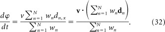This equation suggests that as the rat passes through the peak of the envelope, we should see phase precession (dϕ/dt > 0) if two conditions are satisfied: (1) all weights w_n are positive, and (2) all slopes of speed modulation are positive [that is, d_n,x = v · d_n > 0; this condition is equivalent to the positivity constraint introduced by Burgess (2008)]. In our simulations, the first condition was always satisfied because weight coefficients were set uniformly equal to one. The second condition dictates that the carrier frequency must exceed the base frequency by a greater amount at higher running speeds, and it is satisfied if the absolute angle between the preferred direction vector d_n and the velocity vector v does not exceed 90°. In our simulations of a place cell on the linear track (Fig. 9A,B), we chose VCO vectors that were aligned with the rat's direction of movement on the track, so that d_n,x = v · d_n > 0 was satisfied and phase precession occurred. However, VCO vectors were not always aligned with the rat's movement direction in open field simulations (Fig. 9C), so phase precession did not always occur during spike activity in these simulations (results not shown)

Discussion

Here we recorded theta cells with burst frequencies that varied as the cosine of a rat's allocentric movement direction (Figs. 1–6), and thus appeared to behave like VCOs in oscillatory interference models of path integration (Burgess et al., 2005, 2007; Giocomo et al., 2007; Hasselmo et al., 2007; Blair et al., 2008; Burgess, 2008; Hasselmo, 2008; Zilli and Hasselmo, 2010). Computer simulations demonstrated how grid, place, and border cells could all be formed by a postsynaptic neuron that detects location-dependent synchrony among inputs from theta cells with firing properties similar to those observed in our experiments (Figs. 7–9). These results suggest that populations of theta cells might generate VCO signals from which spatial memories can be synthesized via oscillatory interference.

Theta cells as VCOs

It has been proposed that theta oscillations encoding VCO signals might arise from intrinsic membrane currents within the dendrites of spatially tuned neurons (Kamondi et al., 1998; Lengyel et al., 2003; Burgess et al., 2007; Giocomo et al., 2007; Hasselmo et al., 2007; Losonczy et al. 2010) (but see Remme et al., 2010) or from populations of neurons that fire rhythmically at velocity-modulated frequencies (Blair et al., 2008; Burgess, 2008; Hasselmo, 2008; Zilli et al., 2009; Zilli and Hasselmo, 2010). In the latter case, theory predicts that rhythmic firing should be modulated by a rat's movement direction. It has been shown previously that anterior thalamus contains neurons with firing rates that are modulated by both head direction and theta rhythm (Tsanov et al., 2011a) and that medial septum contains neurons that exhibit maximal theta rhythmicity when a rat runs in a specific direction on a linear track (King et al., 1998). However, our present findings provide the first evidence for theta oscillations that with frequencies that vary as the cosine of a rat's allocentric movement direction, which is absolutely necessary for path integration by oscillatory interference.

Cosine directional tuning was observed in a higher proportion of recording sessions from anterior thalamus (Fig. 2) than medial septum (Fig. 3) or hippocampus (Fig. 4), which may have been a consequence of variable experimental conditions that affected the accuracy of burst frequency measurements, rather than an indicator of functional differences among theta cells recorded in different brain regions (see Results). At the running speeds we observed here, theory predicts that VCO frequencies should vary with movement direction by only fractions of a hertz. To measure theta cell burst frequencies with this level of accuracy, we applied strict criteria for inclusion of session data in the analysis, which unavoidably biased the sample of theta cells we analyzed. Thus, from our present findings, it is difficult to estimate the overall proportion of theta-modulated cells that exhibits directional tuning of their burst frequencies. However, directional modulation of theta cell burst frequencies appeared to be quite prevalent in the structures we targeted, since our reliability threshold for cosine directional tuning was beaten during at least one session by 90% (19 of 21) of the cells admitted for analysis. Moreover, directional tuning followed landmark rotations (Fig. 6), as would be expected for neurons involved in path integration.

Spatial envelopes can only be synthesized from a set of VCOs that are modulated around exactly the same base frequency, and thereby coupled to one another through a shared reference phase (Eq. 17). To test whether different theta cells share a common reference phase, it would be necessary to simultaneously record pairs of theta cells (which was not done here) and show that the offset between their burst phases varies with the rat's position in a manner that forms a 2D cosine grating (Burgess, 2008). Such experiments could provide a critical test of whether theta cells encode VCO signals that share a common reference phase. However, they would be challenging to perform, because only theta cells with sufficiently different preferred vectors (separated by sufficiently long difference vectors) would form gratings with spatial frequencies high enough to observe within the confines of an experimental environment.

Spatial memory coding by theta cells

Computational models have assumed that place cells form their firing fields by summing inputs from grid cells (McNaughton et al., 2006; Solstad et al., 2006; Blair et al., 2007; Gorchetchnikov and Grossberg, 2007; Savelli and Knierim, 2010; Monaco and Abbott, 2011) or boundary vector cells (Hartley et al., 2000). Here, we showed how place cells might instead form by summing direct excitatory or inhibitory inputs from theta cell VCOs (Figs. 7, 9). This does not necessarily conflict with prior models, since grid and boundary vector cells can themselves be synthesized from theta cells (Fig. 9C). Hence, place cells could either receive direct inputs from theta cell VCOs (as in our simulations) or indirect inputs from grid, border, or boundary vector cells (as in prior models) that are each formed by “bundling” several VCOs together. In either case, a place cell which fires over a small region of space would ultimately derive its positional selectivity by detecting rare occurrences of location-dependent synchrony among many VCOs.

Recent studies reported that hexagonal firing patterns of entorhinal grid cells were severely impaired when theta rhythm was disrupted by inactivation of the medial septum (Brandon et al., 2011; Koenig et al., 2011), supporting the possibility that grid cells may derive their positional firing from theta oscillations. However, hippocampal place cells can continue to exhibit spatial firing (and retain some theta modulation of their spike trains) after disruption of ascending theta pathways (Mizumori et al., 1989; Sharp and Koester, 2008; Koenig et al., 2011), after loss of inputs from entorhinal cortex (Van Cauter et al., 2008; Brun et al., 2008a), and before the development of entorhinal grid cells in rat pups (Wills et al., 2010). One explanation for this pattern of findings could be that place cells receive diverse VCO inputs from both direct (e.g., theta cells) and indirect (e.g., grid or boundary vector cells) sources, and any of these inputs may be sufficient to support some degree of spatial firing by place cells after other inputs are lost. Moreover, some inputs may be less susceptible than others to disruptions of theta rhythm. For example, boundary vector cells might derive some of their spatial tuning from sensory signals generated by encounters with landmarks or boundaries, rather than by detecting synchrony among VCOs that perform path integration (O'Keefe and Burgess, 2005; Burgess et al., 2007; Wills et al. 2010).

Anatomical origins of VCO signals

To synthesize diverse populations of spatially tuned neurons from VCOs, identical copies of each VCO signal must be generated at different temporal phase shifts. To satisfy this computational requirement, we conceptualized the VCO circuit as a “ring oscillator” composed from a circular layer of theta cells, each bursting on its own phase of the VCO cycle (Fig. 7B) (Blair et al., 2008). In simulations, we showed how place, grid, and border cells could all be formed by target neurons that detect synchrony among inputs from different theta cells residing in a matrix of such ring oscillators (Fig. 7C).

Evidence suggests that theta oscillations in hippocampus and cortex may be driven and synchronized by subcortical CPGs, which send ascending projections to spatial memory circuits via the medial septum and limbic thalamus (Petsche et al., 1965; Gogolak et al., 1967; Vertes and Kocsis, 1997). These ascending theta pathways exhibit considerable anatomical overlap with ascending head-direction pathways (Vann and Aggleton, 2004; Taube, 2007; Blair et al., 2008; Sharp and Koester, 2008). Interestingly, our ring oscillator model of the theta CPG circuit performs translational path integration in almost exactly the same way that angular path integration is performed by ring attractor models of head-direction cells (Skaggs et al., 1995; Redish et al., 1996; Zhang, 1996; Song and Wang, 2005; Blair et al., 2008). This suggests the intriguing possibility that head-direction signals and velocity-modulated theta rhythm might both emerge from similar subcortical ring attractor circuits and then follow parallel ascending pathways to reach spatial memory circuits in the hippocampus and cortex. To test this, future studies should investigate whether theta cells with directionally tuned burst frequencies can be identified in subcortical structures from which theta rhythm originates.

Neural coding by envelope synthesis

The nervous system generates a multitude of oscillatory rhythms spanning a wide range of frequency bands (Buzsáki, 2006), and phase relationships among such oscillators have been proposed to encode information not only about space, but also about time (Miall, 1989; Hopfield and Brody, 2001; Matell and Meck 2004) or complex sensory stimuli (Laurent et al., 2001; Tiesinga et al., 2008; Koepsell et al., 2010). If the phase of a neural oscillator shifts smoothly in conjunction with a time-varying state variable, x, then that oscillator's frequency would inherently be modulated by dx/dt, and thereby exhibit firing properties analogous to the velocity-modulated theta cells we observed here. In principle, the existence of such oscillators in the nervous system would make it possible to synthesize almost any desired envelope function (as specified by Eqs. 20, 25) in the state space of x, and thereby provide a powerful and flexible mechanism for constructing mental representations in biological neural networks.

References

- Bissiere S, Zelikowsky M, Ponnusamy R, Jacobs N, Blair HT, Fanselow MS. Electrical synapses control hippocampal contributions to fear learning and memory. Science. 2011;331:87–91. doi: 10.1126/science.1193785. [DOI] [PMC free article] [PubMed] [Google Scholar]
- Blair HT, Sharp PE. Anticipatory head direction signals in anterior thalamus: evidence for a thalamocortical circuit that integrates angular head motion to compute head direction. J Neurosci. 1995;15:6260–6270. doi: 10.1523/JNEUROSCI.15-09-06260.1995. [DOI] [PMC free article] [PubMed] [Google Scholar]
- Blair HT, Welday AC, Zhang K. Scale-invariant memory representations emerge from moiré interference between grid fields that produce theta oscillations: a computational model. J Neurosci. 2007;27:3211–3229. doi: 10.1523/JNEUROSCI.4724-06.2007. [DOI] [PMC free article] [PubMed] [Google Scholar]
- Blair HT, Gupta K, Zhang K. Conversion of a phase- to a rate-coded position signal by a three-stage model of theta cells, grid cells, and place cells. Hippocampus. 2008;18:1239–1255. doi: 10.1002/hipo.20509. [DOI] [PMC free article] [PubMed] [Google Scholar]
- Brandon MP, Bogaard AR, Libby CP, Connerney MA, Gupta K, Hasselmo ME. Reduction of theta rhythm dissociates grid cell spatial periodicity from directional tuning. Science. 2011;332:595–599. doi: 10.1126/science.1201652. [DOI] [PMC free article] [PubMed] [Google Scholar]
- Brun VH, Leutgeb S, Wu HQ, Schwarcz R, Witter MP, Moser EI, Moser MB. Impaired spatial representation in CA1 after lesion of direct input from entorhinal cortex. Neuron. 2008a;57:290–302. doi: 10.1016/j.neuron.2007.11.034. [DOI] [PubMed] [Google Scholar]
- Brun VH, Solstad T, Kjelstrup KB, Fyhn M, Witter MP, Moser EI, Moser M-B. Progressive increase in grid scale from dorsal to ventral medial entorhinal cortex. Hippocampus. 2008b;18:1200–1212. doi: 10.1002/hipo.20504. [DOI] [PubMed] [Google Scholar]
- Burgess N. Grid cells and theta as oscillatory interference: theory and predictions. Hippocampus. 2008;18:1157–1174. doi: 10.1002/hipo.20518. [DOI] [PMC free article] [PubMed] [Google Scholar]
- Burgess N, Barry C, O'Keefe J. An oscillatory interference model of grid cell firing. Hippocampus. 2007;17:801–812. doi: 10.1002/hipo.20327. [DOI] [PMC free article] [PubMed] [Google Scholar]
- Burgess N, Barry C, Jeffery KJ, O'Keefe J. A grid and place cell model of path integration utilizing phase precession versus theta. Paper presented 1st Annual conference on Computational Cognitive Neuroscience; November 10–11; Washington, DC. 2005. [Google Scholar]
- Buzsáki G. Rhythms of the brain. New York: Oxford UP; 2006. [Google Scholar]
- Carnevale NT, Hines ML. The NEURON book. Cambridge, UK: Cambridge UP; 2006. [Google Scholar]
- Destexhe A, Mainen ZF, Sejnowski TJ. An efficient method for computing synaptic conductances based on a kinetic model of receptor binding. Neural Comput. 1994;6:10–14. [Google Scholar]
- Düzel E, Penny WD, Burgess N. Brain oscillations and memory. Curr Opin Neurobiol. 2010;20:143–149. doi: 10.1016/j.conb.2010.01.004. [DOI] [PubMed] [Google Scholar]
- Eichenbaum H, Cohen NJ. The hippocampus—what does it do? Behav Neural Biol. 1992;57:2–36. doi: 10.1016/0163-1047(92)90724-i. [DOI] [PubMed] [Google Scholar]
- Etienne AS, Jeffery KJ. Path integration. Hippocampus. 2004;14:180–192. doi: 10.1002/hipo.10173. [DOI] [PubMed] [Google Scholar]
- Freund TF, Antal M. GABA-containing neurons in the septum control inhibitory interneurons in the hippocampus. Nature. 1988;336:170–173. doi: 10.1038/336170a0. [DOI] [PubMed] [Google Scholar]
- Geisler C, Robbe D, Zugaro M, Sirota A, Buzsáki G. Hippocampal place cell assemblies are speed-controlled oscillators. Proc Natl Acad Sci U S A. 2007;104:8149–8154. doi: 10.1073/pnas.0610121104. [DOI] [PMC free article] [PubMed] [Google Scholar]
- Geisler C, Diba K, Pastalkova E, Mizuseki K, Royer S, Buzsáki G. Temporal delays among place cells determine the frequency of population theta oscillations in the hippocampus. Proc Natl Acad Sci U S A. 2010;107:7957–7962. doi: 10.1073/pnas.0912478107. [DOI] [PMC free article] [PubMed] [Google Scholar]
- Giocomo LM, Zilli EA, Fransén E, Hasselmo ME. Temporal frequency of subthreshold oscillations scales with entorhinal grid cell field spacing. Science. 2007;315:1719–1722. doi: 10.1126/science.1139207. [DOI] [PMC free article] [PubMed] [Google Scholar]
- Gogolák G, Petsche H, Sterc J, Stumpf C. Septum cell activity in the rabbit under reticular stimulation. Brain Res. 1967;5:508–510. doi: 10.1016/0006-8993(67)90022-4. [DOI] [PubMed] [Google Scholar]
- Gorchetchnikov A, Grossberg S. Space, time and learning in the hippocampus: how fine spatial and temporal scales are expanded into population codes for behavioral control. Neural Netw. 2007;20:182–193. doi: 10.1016/j.neunet.2006.11.007. [DOI] [PubMed] [Google Scholar]
- Hafting T, Fyhn M, Molden S, Moser MB, Moser EI. Microstructure of a spatial map in the entorhinal cortex. Nature. 2005;436:801–806. doi: 10.1038/nature03721. [DOI] [PubMed] [Google Scholar]
- Hartley T, Burgess N, Lever C, Cacucci F, O'Keefe J. Modeling place fields in terms of the cortical inputs to the hippocampus. Hippocampus. 2000;10:369–379. doi: 10.1002/1098-1063(2000)10:4<369::AID-HIPO3>3.0.CO;2-0. [DOI] [PubMed] [Google Scholar]
- Hartmann WM. Signals, sound, and sensation. New York: Springer; 1998. [Google Scholar]
- Harvey CD, Collman F, Dombeck DA, Tank DW. Intracellular dynamic of hippocampal place cells during virtual navigation. Nature. 2009;461:941–946. doi: 10.1038/nature08499. [DOI] [PMC free article] [PubMed] [Google Scholar]
- Hasselmo ME. Grid cell mechanisms and function: contributions of entorhinal persistent spiking and phase resetting. Hippocampus. 2008;18:1213–1229. doi: 10.1002/hipo.20512. [DOI] [PMC free article] [PubMed] [Google Scholar]
- Hasselmo ME, Giocomo LA, Zilli EA. Grid cell firing may arise from interference of theta frequency membrane potential oscillations in single neurons. Hippocampus. 2007;17:1252–1271. doi: 10.1002/hipo.20374. [DOI] [PMC free article] [PubMed] [Google Scholar]
- Hasselmo ME, Giocomo LM, Brandon MP, Yoshida M. Cellular dynamical mechanisms for encoding the time and place of events along spatiotemporal trajectories in episodic memory. Behav Brain Res. 2010;215:261–274. doi: 10.1016/j.bbr.2009.12.010. [DOI] [PMC free article] [PubMed] [Google Scholar]
- Hines ML, Morse T, Migliore M, Carnevale NT, Shepherd GM. ModelDB: a database to support computational neuroscience. J. Comput. Neurosci. 2004;17:7–11. doi: 10.1023/B:JCNS.0000023869.22017.2e. [DOI] [PMC free article] [PubMed] [Google Scholar]
- Hopfield JJ, Brody CD. What s a moment? Transient synchrony as a collective mechanism for spatiotemporal integration. Proc Natl Acad U S A. 2001;98:128207. doi: 10.1073/pnas.031567098. [DOI] [PMC free article] [PubMed] [Google Scholar]
- Jeewajee A, Barry C, O'Keefe J, Burgess N. Grid cells and theta as oscillatory interference: electrophysiological data from freely moving rats. Hippocampus. 2008a;18:1175–1185. doi: 10.1002/hipo.20510. [DOI] [PMC free article] [PubMed] [Google Scholar]
- Jeewajee A, Lever C, Burton S, O'Keefe J, Burgess N. Environmental novelty is signaled by reduction of the hippocampal theta frequency. Hippocampus. 2008b;18:340–348. doi: 10.1002/hipo.20394. [DOI] [PMC free article] [PubMed] [Google Scholar]
- Jones EG. The thalamus. New York: Plenum; 1985. [Google Scholar]
- Kamondi A, Acsády L, Wang XJ, Buzsáki G. Theta oscillations in somata and dendrites of hippocampal pyramidal cells in vivo: activity-dependent phase precession of action potentials. Hippocampus. 1998;8:244–261. doi: 10.1002/(SICI)1098-1063(1998)8:3<244::AID-HIPO7>3.0.CO;2-J. [DOI] [PubMed] [Google Scholar]
- King C, Recce M, O'Keefe J. The rhythmicity of cells of the medial septum/diagonal band of Broca in the awake freely moving rat: relationships with behavior and hippocampal theta. Eur J Neurosci. 1998;10:464–477. doi: 10.1046/j.1460-9568.1998.00026.x. [DOI] [PubMed] [Google Scholar]
- Knierim JJ, Kudrimoti HS, McNaughton BL. Place cells, head direction cells, and the learning of landmark stability. J Neurosci. 1995;15:1648–1659. doi: 10.1523/JNEUROSCI.15-03-01648.1995. [DOI] [PMC free article] [PubMed] [Google Scholar]
- Knierim JJ, Kudrimoti HS, McNaughton BL. Interactions between idiothetic cues and external landmarks in the control of place cells and head direction cells. J Neurophysiol. 1998;80:425–446. doi: 10.1152/jn.1998.80.1.425. [DOI] [PubMed] [Google Scholar]
- Koenig J, Linder AN, Leutgeb JK, Leutgeb S. The spatial periodicity of grid cells is not sustained during reduced theta oscillations. Science. 2011;332:592–595. doi: 10.1126/science.1201685. [DOI] [PubMed] [Google Scholar]
- Koepsell K, Wang X, Hirsch JA, Sommer FT. Exploring the function of neural oscillations in early sensory systems. Front Neurosci. 2010;4:53. doi: 10.3389/neuro.01.010.2010. [DOI] [PMC free article] [PubMed] [Google Scholar]
- Laurent G, Stopfer M, Friedrich RW, Rabinovich MI, Volkovskii A, Abarbanel HD. Odor encoding as an active, dynamical process: experiments, computation, and theory. Ann Rev Neurosci. 2001;24:263–297. doi: 10.1146/annurev.neuro.24.1.263. [DOI] [PubMed] [Google Scholar]
- Lengyel M, Szatmáry Z, Erdi P. Dynamically detuned oscillations account for the coupled rate and temporal code of place cell firing. Hippocampus. 2003;13:700–714. doi: 10.1002/hipo.10116. [DOI] [PubMed] [Google Scholar]
- Leutgeb JK, Leutgeb S, Moser MB, Moser EI. Pattern separation in the dentate gyrus and CA3 of the hippocampus. Science. 2007;315:961–966. doi: 10.1126/science.1135801. [DOI] [PubMed] [Google Scholar]
- Lever C, Burton S, Jeewajee A, O'Keefe J, Burgess N. Boundary vector cells in the subiculum of the hippocampal formation. J Neurosci. 2009;29:9771–9777. doi: 10.1523/JNEUROSCI.1319-09.2009. [DOI] [PMC free article] [PubMed] [Google Scholar]
- Losonczy A, Zemelman BV, Vaziri A, Magee JC. Network mechanisms of theta related neuronal activity in hippocampal CA1 pyramidal neurons. Nat Neurosci. 2010;13:967–972. doi: 10.1038/nn.2597. [DOI] [PMC free article] [PubMed] [Google Scholar]
- Lubenov EV, Siapas AG. Hippocampal theta oscillations are travelling waves. Nature. 2009;459:534–539. doi: 10.1038/nature08010. [DOI] [PubMed] [Google Scholar]
- Matell MS, Meck WH. Cortico-striatal circuits and interval timing: coincidence detection of oscillatory processes. Brain Res Cogn Brain Res. 2004;21:139–170. doi: 10.1016/j.cogbrainres.2004.06.012. [DOI] [PubMed] [Google Scholar]
- McNaughton BL, Barnes CA, Gerrard JL, Gothard K, Jung MW, Knierim JJ, Kudrimoti H, Qin Y, Skaggs WE, Suster M, Weaver KL. Deciphering the hippocampal polyglot: the hippocampus as a path integration system. J Exp Biol. 1996;199:173–185. doi: 10.1242/jeb.199.1.173. [DOI] [PubMed] [Google Scholar]
- McNaughton BL, Battaglia FP, Jensen O, Moser EI, Moser MB. Path integration and the neural basis of the “cognitive map.”. Nat Rev Neurosci. 2006;7:663–678. doi: 10.1038/nrn1932. [DOI] [PubMed] [Google Scholar]
- Mhatre H, Gorchetchnikov A, Grossberg S. Grid cell hexagonal patterns formed by fast self-organized learning within entorhinal cortex. Hippocampus. 2010 doi: 10.1002/hipo.20901. Advance online publication. doi: 10.1002/hipo.20901. [DOI] [PubMed] [Google Scholar]
- Miall C. The storage of time intervals using oscillating neurons. Neural Comput. 1989;1:359–371. [Google Scholar]
- Mizumori SJ, McNaughton BL, Barnes CA, Fox KB. Preserved spatial coding in hippocampal CA1 pyramidal cells during reversible suppression of CA3c output: evidence for pattern completion in hippocampus. J Neurosci. 1989;9:3915–3928. doi: 10.1523/JNEUROSCI.09-11-03915.1989. [DOI] [PMC free article] [PubMed] [Google Scholar]
- Monaco JD, Abbott LR. Modular realignment of entorhinal grid cell activity as a basis for hippocampal remapping. J Neurosci. 2011;31:9414–9425. doi: 10.1523/JNEUROSCI.1433-11.2011. [DOI] [PMC free article] [PubMed] [Google Scholar]
- Muller RU, Kubie JL. The effects of changes in the environment on the spatial firing of hippocampal complex-spike cells. J Neurosci. 1987;7:1951–1968. doi: 10.1523/JNEUROSCI.07-07-01951.1987. [DOI] [PMC free article] [PubMed] [Google Scholar]
- O'Keefe J, Burgess N. Dual phase and rate coding in hippocampal place cells: theoretical significance and relationship to entorhinal grid cells. Hippocampus. 2005;15:853–866. doi: 10.1002/hipo.20115. [DOI] [PMC free article] [PubMed] [Google Scholar]
- O'Keefe J, Dostrovsky J. The hippocampus as a spatial map. Preliminary evidence from unit activity in the freely-moving rat. Brain Res. 1971;34:171–175. doi: 10.1016/0006-8993(71)90358-1. [DOI] [PubMed] [Google Scholar]
- O'Keefe J, Nadel L. The hippocampus as a cognitive map. New York: Oxford UP; 1978. [Google Scholar]
- O'Keefe J, Recce ML. Phase relationship between hippocampal place units and the EEG theta rhythm. Hippocampus. 1993;3:317–330. doi: 10.1002/hipo.450030307. [DOI] [PubMed] [Google Scholar]
- Paxinos G, Watson C. The rat brain in stereotaxic coordinates. Sydney: Academic; 1997. [DOI] [PubMed] [Google Scholar]
- Petsche H, Gogolak G, Vanzwieten PA. Rhythmicity of septal cell discharges at various levels of reticular excitation. Electroencephalogr Clin Neurophysiol. 1965;19:25–33. doi: 10.1016/0013-4694(65)90004-0. [DOI] [PubMed] [Google Scholar]
- Ranck JB., Jr Studies on single neurons in dorsal hippocampal formation and septum in unrestrained rats. I. Behavioral correlates and firing repertoires. Exp Neurol. 1973;41:461–531. doi: 10.1016/0014-4886(73)90290-2. [DOI] [PubMed] [Google Scholar]
- Redish AD, Elga AN, Touretzky DS. A coupled attractor model of the rodent head-direction system. Network. 1996;7:671–685. [Google Scholar]
- Remme MW, Lengyel M, Gutkin BS. Democracy-independence trade-off in oscillating dendrites and its implications for grid cells. Neuron. 2010;66:429–437. doi: 10.1016/j.neuron.2010.04.027. [DOI] [PMC free article] [PubMed] [Google Scholar]
- Rivas J, Gatztelu JM, García-Austt E. Changes in hippocampal cell discharge patterns and theta rhythm spectral properties as a function of walking velocity in the guinea pig. Exp Brain Res. 1996;108:113–118. doi: 10.1007/BF00242908. [DOI] [PubMed] [Google Scholar]
- Rutishauser U, Ross IB, Mamelak AN, Schuman EM. Human memory strength is predicted by theta-frequency phase locking of single neurons. Nature. 2010;464:903–907. doi: 10.1038/nature08860. [DOI] [PubMed] [Google Scholar]
- Sargolini F, Fyhn M, Hafting T, McNaughton BL, Witter MP, Moser MB, Moser EI. Conjunctive representation of position, direction, and velocity in entorhinal cortex. Science. 2006;312:758–762. doi: 10.1126/science.1125572. [DOI] [PubMed] [Google Scholar]
- Savelli F, Knierim JJ. Hebbian analysis of the transformation of medial entorhinal grid-cell inputs to hippocampal place fields. J. Neurophysiol. 2010;103:3167–3183. doi: 10.1152/jn.00932.2009. [DOI] [PMC free article] [PubMed] [Google Scholar]
- Savelli F, Yoganarasimha D, Knierim JJ. Influence of boundary removal on the spatial representations of the medial entorhinal cortex. Hippocampus. 2008;18:1270–1282. doi: 10.1002/hipo.20511. [DOI] [PMC free article] [PubMed] [Google Scholar]
- Sharp PE, Koester K. Lesions of the mammillary body region severely disrupt the cortical head direction, but not place cell signal. Hippocampus. 2008;18:766–784. doi: 10.1002/hipo.20436. [DOI] [PubMed] [Google Scholar]
- Skaggs WE, Knierim JJ, Kudrimoti HS, McNaughton BL. A model of the neural basis of the rat's sense of direction. Adv Neural Inf Process Syst. 1995;7:173–180. [PubMed] [Google Scholar]
- Skaggs WE, McNaughton BL, Gothard KM, Markus EJ. An information-theoretic approach to deciphering the hippocampal code. Adv Neural Inf Process Syst. 1993;5:1030–1037. [Google Scholar]
- Solstad T, Moser EI, Einevoll GT. From grid cells to place cells: a mathematical model. Hippocampus. 2006;16:1026–1031. doi: 10.1002/hipo.20244. [DOI] [PubMed] [Google Scholar]
- Solstad T, Boccara CN, Kropff E, Moser MB, Moser EI. Representation of geometric borders in the entorhinal cortex. Science. 2008;322:1865–1868. doi: 10.1126/science.1166466. [DOI] [PubMed] [Google Scholar]
- Song P, Wang XJ. Angular path integration by moving “hill of activity”: a spiking neuron model without recurrent excitation of the head-direction system. J Neurosci. 2005;25:1002–1014. doi: 10.1523/JNEUROSCI.4172-04.2005. [DOI] [PMC free article] [PubMed] [Google Scholar]
- Squire LR, Schacter DL, editors. Neuropsychology of memory. Ed 3. New York: Guilford; 2002. [Google Scholar]
- Taube JS. The head direction signal: origins and sensorimotor integration. Annu Rev Neurosci. 2007;30:181–207. doi: 10.1146/annurev.neuro.29.051605.112854. [DOI] [PubMed] [Google Scholar]
- Taube JS, Muller RU, Ranck JB., Jr Head direction cells recorded from the postsubiculum in freely moving rats. II. Effects of environmental manipulations. J Neurosci. 1990;10:436–437. doi: 10.1523/JNEUROSCI.10-02-00436.1990. [DOI] [PMC free article] [PubMed] [Google Scholar]
- Tiesinga P, Fellous JM, Sejnowski TJ. Regulation of spike timing in visual cortical circuits. Nat Rev Neurosci. 2008;9:97–107. doi: 10.1038/nrn2315. [DOI] [PMC free article] [PubMed] [Google Scholar]
- Tsanov M, Chah E, Vann SD, Reilly RB, Erichsen JT, Aggleton JP, O'Mara SM. Theta-modulated head direction cells in the rat anterior thalamus. J Neurosci. 2011a;31:9489–9502. doi: 10.1523/JNEUROSCI.0353-11.2011. [DOI] [PMC free article] [PubMed] [Google Scholar]
- Tsanov M, Chah E, Wright N, Vann SD, Reilly R, Erichsen JT, Aggleton JP, O'Mara SM. Oscillatory entrainment of thalamic neurons by theta rhythm in freely moving rats. J Neurophysiol. 2011b;105:4–17. doi: 10.1152/jn.00771.2010. [DOI] [PMC free article] [PubMed] [Google Scholar]
- Uebachs M, Opitz T, Royeck M, Dickhof G, Horstmann MT, Isom LL, Beck H. Efficacy loss of the anticonvulsant carbamazepine in mice lacking sodium channel beta subunits via paradoxical effects on persistent sodium currents. J Neurosci. 2010;30:8489–8501. doi: 10.1523/JNEUROSCI.1534-10.2010. [DOI] [PMC free article] [PubMed] [Google Scholar]
- Van Cauter T, Poucet B, Save E. Unstable CA1 place cell representation in rats with entorhinal cortex lesions. Eur J Neurosci. 2008;27:1933–1946. doi: 10.1111/j.1460-9568.2008.06158.x. [DOI] [PubMed] [Google Scholar]
- Vann SD, Aggleton JP. The mammillary bodies: two memory systems in one? Nat Rev Neurosci. 2004;5:35–44. doi: 10.1038/nrn1299. [DOI] [PubMed] [Google Scholar]
- Vertes RP, Kocsis B. Brainstem-diencephalo-septohippocampal systems controlling the theta rhythm of the hippocampus. Neuroscience. 1997;81:893–926. doi: 10.1016/s0306-4522(97)00239-x. [DOI] [PubMed] [Google Scholar]
- Wills TJ, Cacucci F, Burgess N, O'Keefe J. Development of the hippocampal cognitive map in preweanling rats. Science. 2010;328:1573–1576. doi: 10.1126/science.1188224. [DOI] [PMC free article] [PubMed] [Google Scholar]
- Zhang K. Representation of spatial orientation by the intrinsic dynamics of the head-direction cell ensemble: a theory. J Neurosci. 1996;16:2112–2126. doi: 10.1523/JNEUROSCI.16-06-02112.1996. [DOI] [PMC free article] [PubMed] [Google Scholar]
- Zilli EA, Hasselmo ME. Coupled noisy spiking neurons as velocity-controlled oscillators in a model of grid cell spatial firing. J Neurosci. 2010;30:13850–13860. doi: 10.1523/JNEUROSCI.0547-10.2010. [DOI] [PMC free article] [PubMed] [Google Scholar]
- Zilli EA, Yoshida M, Tahvildari B, Giocomo LM, Hasselmo ME. Evaluation of the oscillatory interference model of grid cell firing through analysis and measured period variance of some biological oscillators. PLoS Comput Biol. 2009;5:e1000573. doi: 10.1371/journal.pcbi.1000573. [DOI] [PMC free article] [PubMed] [Google Scholar]