Mathematical analysis of multiscale models for hepatitis C virus dynamics under therapy with direct-acting antiviral agents

Abstract

Chronic hepatitis C virus (HCV) infection remains a world-wide public health problem. Therapy with interferon and ribavirin leads to viral elimination in less than 50% of treated patients. New treatment options aiming at a higher cure rate are focused on direct-acting antiviral agents (DAAs), which directly interfere with different steps in the HCV life cycle. In this paper, we describe and analyze a recently developed multiscale model that predicts HCV dynamics under therapy with DAAs. The model includes both intracellular viral RNA replication and extracellular viral infection. We calculate the steady states of the model and perform a detailed stability analysis. With certain assumptions we obtain analytical approximations of the viral load decline after treatment initiation. One approximation agrees well with the prediction of the model, and can conveniently be used to fit patient data and estimate parameter values. We also discuss other possible ways to incorporate intracellular viral dynamics into the multiscale model.

1 Introduction

Hepatitis C virus (HCV) infection is a major cause of chronic liver disease, liver cirrhosis and liver cancer. Approximately 130 to 170 million people are chronically infected with HCV in the world [1]. A combination of pegylated interferon (PEG-IFN) and ribavirin (RBV) has been used to treat HCV infection but only led to sustained viral elimination in less than 50% of treated patients infected with HCV genotype 1, the major genotype affecting North America and Europe [2]. New treatment options are focused on the development of direct-acting antiviral agents (DAAs), which directly interfere with different steps in the HCV life cycle [3, 4]. Several important targets are the HCV-encoded protease, polymerase, and NS5A protein [5, 6]. A number of protease and polymerase inhibitors have been developed [7, 8]. Among them, two protease inhibitors, telaprevir and boceprevir, have been approved by the US Food and Drug Administration (FDA) to treat HCV infection when used in combination with PEG-IFN/RBV. In addition, daclatasvir has been identified as an HCV NS5A inhibitor using an innovative screening approach [9]. A second generation of protease inhibitors, such as danoprevir [10, 11], presenting better safety and resistance profiles, are also in clinical evaluation [12, 13]. Although the specific mechanisms of action of some DAAs are not fully understood, they have shown potent antiviral activities in patients infected with HCV genotype 1 [8].

Mathematical models have been developed to study HCV dynamics under therapy [14–16]. In most patients, after treatment is initiated with IFN a biphasic decline in HCV RNA is observed. To understand this decline, a basic viral dynamic model was used to explore the mechanism of action of IFN against HCV [17]. Using this model, it was shown that IFN acts mainly to reduce viral production per infected cell. Consequently, the early viral decline in plasma observed after IFN administration reflects the viral clearance rate, which was estimated to be approximately 6 day⁻¹ [17]. It was also suggested that the variation in the estimates of the infected cell death rate from patient to patient might reflect their differences in cellular immunity [17]. The antiviral mechanisms of action of RBV against HCV have not been fully elucidated. Several mechanisms have been proposed [18, 19] and mathematical models have been used to test these mechanisms. In one study [20], Herrmann et al. developed a model assuming that RBV serves as an immune modulator. In another study [21], Dixit et al. tested the hypothesis that RBV may act by lowering the infectivity of HCV, possibly via mutagenesis. The model in [21] showed that RBV does not influence the first phase viral decline, but increases the slope of the second phase decline in a dose-dependent manner if the efficacy of IFN is low. When the efficacy of IFN is high, RBV does not influence the second phase decline either. These predictions are in agreement with experimental results and can resolve the seemingly conflicting observations that RBV influences the second phase viral decline in some patients but not in others [19, 20, 22].

Most models in the literature treat the infected cell as a “black box” which produces new virions after infection, without considering the intracellular viral RNA replication/degradation within the infected cell [23]. However, these intracellular processes might be important in studying HCV dynamics under DAA therapy because they are directly targeted by DAAs. In this paper, we describe and mathematically analyze a recently developed multiscale model that studies the dynamics of HCV infection under therapy with DAAs [24, 25]. The model includes both intracellular viral RNA replication/degradation and extracellular viral infection. We calculate the steady states of the model and provide a detailed stability analysis. With certain assumptions we approximate the viral load decline after treatment initiation. These approximations have been used to analyze viral load data from patients treated with DAAs such as the NS5A inhibitor daclatasvir [24] and the protease inhibitors telaprevir [24] and danoprevir [25]. We perform numerical simulations to illustrate the effects of DAA's different antiviral actions on the viral load change during therapy. We also discuss other possible ways to incorporate intracellular viral dynamics into the multiscale model.

2 Model description

The basic viral dynamic model used to study HCV dynamics under IFN-based therapy includes three variables [17]: uninfected target cells (T ), productively infected cells (I), and free virus (V). The parameters s and d are the production rate and per capita death rate of target cells, respectively. Viral infection is assumed to occur at a rate βV T. Productively infected cells are lost, by either natural death or immune attack, at rate δ per cell. Virus is released from productively infected cells at rate p per cell and is cleared at rate c per virion. IFN therapy was shown to mainly reduce viral production [17], with efficacy ∊. The model can be described by the following equations:

$$\begin{array}{cc}\hfill & \frac{d}{\mathit{dt}}T=s-\beta \mathit{VT}-\mathit{dT},\hfill \\ \hfill & \frac{d}{\mathit{dt}}I=\beta \mathit{VT}-\delta I,\hfill \\ \hfill & \frac{d}{\mathit{dt}}V=(1-∊)\mathit{pI}-\mathit{cV},\hfill \end{array}$$ (1)

We extend the model by incorporating another variable, R, which represents the quantity of intracellular genomic RNA (i.e., positive-strand HCV RNA) within an infected cell. The dynamics of intracellular viral RNA are determined by RNA production and loss due to degradation and assembly/secretion as virions into plasma. A simple model of intracellular viral RNA dynamics in an infected cell is described by the equation

$$\frac{\mathit{dR}}{\mathit{da}}=\alpha \left(a\right)-\left[\rho \right(a)+\mu (a\left)\right]R\left(a\right),$$ (2)

where a is the age of infection, i.e., the time that has elapsed since an HCV virion, which contains a single viral RNA genome, has entered the cell. The parameters α, μ and ρ are assumed to be age-dependent rates of intracellular viral RNA production, degradation, and assembly/secretion, respectively. We also assume that a cell is infected by a single virion initially and hence there is only one viral RNA in an infected cell at age 0, i.e., R(0) = 1.

Combining Eqs. (1) and (2), we obtain a multiscale model including both intracellular viral RNA replication and extracellular viral infection dynamics, described by the following partial differential equations (PDEs):

$$\begin{array}{cc}\hfill & \frac{d}{\mathit{dt}}T\left(t\right)=s-\beta V\left(t\right)T\left(t\right)-\mathit{dT}\left(t\right),\hfill \\ \hfill & \frac{\partial }{\partial t}I(a,t)+\frac{\partial }{\partial a}I(a,t)=-\delta \left(a\right)I(a,t),\hfill \\ \hfill & I(0,t)=\beta V\left(t\right)T\left(t\right),I(a,0)=I_0\left(a\right),\hfill \\ \hfill & \frac{\partial }{\partial t}R(a,t)+\frac{\partial }{\partial a}R(a,t)=\alpha \left(a\right)-\left[\rho \right(a)+\mu (a\left)\right]R(a,t),\hfill \\ \hfill & R(0,t)=1,R(a,0)=R_0\left(a\right),\hfill \\ \hfill & \frac{d}{\mathit{dt}}V\left(t\right)={\int }_0^{\infty }\rho \left(a\right)R(a,t)I(a,t)\mathit{da}-\mathit{cV}\left(t\right),\hfill \end{array}$$ (3)

where I₀(a) and R₀(a) are the initial distributions of infected cells and intracellular viral RNA, respectively.

Therapy with DAAs may inhibit intracellular viral RNA production, block assembly/secretion as virus into plasma, and/or enhance RNA degradation. We assume the efficacies of these actions are ∊_α, ∊_s, and κ, respectively, where 0 ≤ ∊_α, ∊_s ≤ 1 and κ ≥ 1. We further assume the viral infection has reached steady-state at the time therapy is initiated. The multiscale model under therapy then becomes

$$\begin{array}{cc}\hfill & \frac{d}{\mathit{dt}}T\left(t\right)=s-\mathit{dT}\left(t\right)-\beta V\left(t\right)T\left(t\right),\hfill \\ \hfill & \frac{\partial }{\partial t}I(a,t)+\frac{\partial }{\partial a}I(a,t)-\delta \left(a\right)I(a,t),\hfill \\ \hfill & I(0,t)=\beta V\left(t\right)T\left(t\right),I(a,0)=\stackrel{‒}{I}\left(a\right),\hfill \\ \hfill & \frac{\partial }{\partial t}R(a,t)+\frac{\partial }{\partial a}R(a,t)=(1-{∊}_s)\alpha \left(a\right)-\left[\right(1-{∊}_s\left)\rho \right(a)+\kappa \mu (a\left)\right]R(a,t),\hfill \\ \hfill & R(0,t)=1,R(a,0)=\stackrel{‒}{R}\left(a\right),\hfill \\ \hfill & \frac{d}{\mathit{dt}}V\left(t\right)=(1-{∊}_s){\int }_0^{\infty }\rho \left(a\right)R(a,t)I(a,t)\mathit{da}-\mathit{cV}\left(t\right),\hfill \end{array}$$ (4)

where t = 0 is the time at which treatment is initiated. $\stackrel{‒}{I}\left(a\right)$ and $\stackrel{‒}{R}\left(a\right)$ are the steady-state distributions of infected cells and intracellular viral RNA, respectively, before therapy.

3 Model analysis

We calculate the steady states of the pre-therapy model (3) and study their stability.

Let

$$\omega \left(a\right)=e^{-{\int }_0^a}\delta \left(\tau \right)d\tau \text{and}\pi \left(a\right)=e^{-{\int }_0^a}\left[\rho \right(\tau )+\mu (\tau \left)\right]d\tau ,$$ (5)

where ω(a) and π(a) can be interpreted as the probability of an infected cell and an intracellular viral RNA surviving to age a (of the infected cell), respectively. At steady state, the density of infected cells of age a is

$$\stackrel{‒}{I}\left(a\right)=\stackrel{‒}{I}\left(0\right)\omega \left(a\right)=\beta \stackrel{‒}{V}\stackrel{‒}{T}\omega \left(a\right),$$ (6)

where $\stackrel{‒}{V}$ and $\stackrel{‒}{T}$ are the steady-state viral load and target cell density, respectively. The steady state of the intracellular viral RNA level within an infected cell of age a is given by the solution of Eq. (2) with R(0) = 1, i.e.,

$$\stackrel{‒}{R}\left(a\right)=\pi \left(a\right)+{\int }_0^a\frac{\pi \left(a\right)}{\pi \left(u\right)}\alpha \left(u\right)\mathit{du}.$$ (7)

When δ(a), α(a), ρ(a), and μ(a) are all assumed to be constant, we have ω(a) = e^−δa, π(a) = e^−(ρ+μ)a, and

$$\stackrel{‒}{I}\left(a\right)=\beta \stackrel{‒}{V}\stackrel{‒}{T}{e}^{-\delta a},\stackrel{‒}{R}\left(a\right)=\frac{\alpha }{\rho +\mu }+(1-\frac{\alpha }{\rho +\mu })e^{-(\rho +\mu )a}.$$ (8)

Plugging the steady states $\stackrel{‒}{I}\left(a\right)$ and $\stackrel{‒}{R}\left(a\right)$ in (6) and (7) into the V equation in (3), we have

$${\int }_0^{\infty }\rho \left(a\right)\stackrel{‒}{R}\left(a\right)\beta \stackrel{‒}{V}\stackrel{‒}{T}\omega \left(a\right)\mathit{da}=c\stackrel{‒}{V}.$$ (9)

Let

$$N={\int }_0^{\infty }\rho \left(a\right)\stackrel{‒}{R}\left(a\right)\omega \left(a\right)\mathit{da}.$$ (10)

Thus, N gives the total number of virions produced by one infected cell during its lifetime. This number is called the viral burst size [26]. Solving Eq. (9) for $\stackrel{‒}{T}$ and using N in (10), we obtain

$$\stackrel{‒}{T}=\frac{c}{\beta N}.$$

From the first equation of (3), we obtain the steady-state viral load,

$$\stackrel{‒}{V}=\frac{\beta Ns-\mathit{dc}}{\beta c}.$$

Substituting $\stackrel{‒}{V}$ and $\stackrel{‒}{T}$ into Eq. (6), we obtain

$$\stackrel{‒}{I}\left(a\right)=\frac{\beta Ns-\mathit{dc}}{\beta N}\omega \left(a\right).$$

Let

$${\mathcal{R}}_0=\frac{\beta Ns}{\mathit{dc}}.$$ (11)

${\mathcal{R}}_0$ is the basic reproductive ratio of model (3), where s/d is the target cell density at the start of infection [27]. Obviously, the infected steady state ($\stackrel{‒}{T}$, $\stackrel{‒}{I}\left(a\right)$, $\stackrel{‒}{R}\left(a\right)$, $\stackrel{‒}{V}$) of model (3) is feasible, i.e., has all variables positive, if and only if ${\mathcal{R}}_0>1$. The infection-free steady state is (s/d, 0, $\stackrel{‒}{R}\left(a\right)$, 0).

Using the method of characteristics, we can obtain a complete solution for R(a, t) and I(a, t). The characteristic curves are t − a = constant. We assume that they intersect with the age-axis at (a₀, 0) and intersect with the time-axis at (0, t₀), where a₀ ≥ 0 and t₀ ≥ 0.

When a ≥ t, the characteristic curves can be described by the parametric equation t = τ, a = τ + a₀, where τ is a free parameter. When τ increases from 0 to t, a(τ) increases from a₀ to a and t(τ) increases from 0 to t. Along the characteristic curves, we have

$$\frac{\mathit{dR}\left(a\right(\tau ),t(\tau \left)\right)}{d\tau }=\frac{\partial R}{\partial t}\frac{\mathit{dt}}{d\tau }+\frac{\partial R}{\partial a}\frac{\mathit{da}}{d\tau }=\alpha \left(a\right(\tau \left)\right)-\left[\rho \right(a\left(\tau \right))+\mu (a\left(\tau \right)\left)\right]R\left(a\right(\tau ),t(\tau \left)\right).$$ (12)

This is an ordinary differential equation (ODE) with the independent variable τ.

Using the variation of constants formula, we obtain

$$R(a,t)=R(a_0,0)e^{-{\int }_0^t\left[\rho \right(a\left(\tau \right))+\mu (a\left(\tau \right)\left)\right]d\tau }+e^{-{\int }_0^t\left[\rho \right(a\left(\tau \right))+\mu (a\left(\tau \right)\left)\right]d\tau }{\int }_0^t\alpha \left(a\right(u\left)\right)e^{{\int }_0^u\left[\rho \right(a\left(\tau \right))+\mu (a\left(\tau \right)\left)\right]d\tau }\mathit{du}.$$

Note that

$${\int }_0^t\left[\rho \right(a\left(\tau \right))+\mu (a\left(\tau \right)\left)\right]d\tau ={\int }_{a_0}^a\left[\rho \right(\varsigma )+\mu (\varsigma \left)\right]d\varsigma ,$$

thus we have

$$e^{-{\int }_0^t\left[\rho \right(a\left(\tau \right))+\mu (a\left(\tau \right)\left)\right]d\tau }=e^{-{\int }_{a_0}^a\left[\rho \right(\varsigma )+\mu (\varsigma \left)\right]d\varsigma }=\frac{\pi \left(a\right)}{\pi \left(a_0\right)},$$

where π(a) is defined in Eq. (5).

We also have

$$\begin{array}{c}\hfill \hfill \\ \hfill {\int }_0^t\alpha \left(a\right(u\left)\right)e^{{\int }_0^u\left[\rho \right(a\left(\tau \right))+\mu (a\left(\tau \right)\left)\right]d\tau }\mathit{du}={\int }_0^t\alpha \left(a\right(u\left)\right)e^{{\int }_{a_0}^{a_0+u}\left[\rho \right(\eta )+\mu (\tau \left)\right]d\eta }\mathit{du}\hfill \\ \hfill {\int }_{a_0}^a\alpha \left(\varsigma \right)e^{{\int }_{a_0}^{\varsigma }\left[\rho \right(\eta )+\mu (\eta \left)\right]d\eta }d\varsigma ={\int }_{a_0}^a\alpha \left(\varsigma \right)\frac{\pi \left(a_0\right)}{\pi \left(\varsigma \right)}d\varsigma .\hfill \end{array}$$

Thus, when a ≥ t, we obtain

$$R(a,t)=R(a_0,0)\frac{\pi \left(a\right)}{\pi \left(a_0\right)}+{\int }_{a_0}^a\frac{\pi \left(a\right)}{\pi \left(\varsigma \right)}\alpha \left(\varsigma \right)d\varsigma =R_0(a-t)\frac{\pi \left(a\right)}{\pi (a-t)}+{\int }_0^t\frac{\pi \left(a\right)}{\pi (a-u)}\alpha (a-u)\mathit{du}.$$

When a < t, the characteristic curves can be described by t = τ, a = τ − t₀. When τ increases from t₀ to t, a(τ) increases from 0 to a and t(τ) increases from t₀ to t. Along the characteristic curves, we have the same ODE given by Eq. (12). Using the variation of constants formula again, we obtain

$$R(a,t)=R(0,t_0)e^{-{\int }_{t_0}^t\left[\rho \right(a\left(\tau \right))+\mu (a\left(\tau \right)\left)\right]d\tau }+e^{-{\int }_{t_0}^t\left[\rho \right(a\left(\tau \right))+\mu (a\left(\tau \right)\left)\right]d\tau }{\int }_{t_0}^t\alpha \left(a\right(u\left)\right)e^{{\int }_{t_0}^u\left[\rho \right(a\left(\tau \right))+\mu (a\left(\tau \right)\left)\right]d\tau }\mathit{du}.$$

Note that

$$e^{-{\int }_{t_0}^t\left[\rho \right(a\left(\tau \right))+\mu (a\left(\tau \right)\left)\right]d\tau }=e^{-{\int }_0^a\left[\rho \right(\varsigma )+\mu (\varsigma \left)\right]d\varsigma }=\pi \left(a\right)$$

and

$$\begin{array}{cc}\hfill {\int }_{t_0}^t\alpha (a& \left(u\right))e^{{\int }_{t_0}^u\left[\rho \right(a\left(\tau \right))+\mu (a\left(\tau \right)\left)\right]d\tau }\mathit{du}={\int }_{t_0}^t\alpha (a\left(u\right))e^{{\int }_0^{u-t_0}\left[\rho \right(\eta )+\mu (\eta \left)\right]d\eta }\mathit{du}\hfill \\ \hfill & ={\int }_{t_0}^t\frac{\alpha (u-t_0)}{\pi (u-t_0)}\mathit{du}={\int }_0^{t-t_0}\frac{\alpha \left(\varsigma \right)}{\pi \left(\varsigma \right)}d\varsigma ={\int }_0^a\frac{a\left(\varsigma \right)}{\pi \left(\varsigma \right)}d\varsigma .\hfill \end{array}$$

Thus, when a < t, we have

$$R(a,t)=R(0,t-a)\pi \left(a\right)+{\int }_0^a\frac{\pi \left(a\right)}{\pi \left(u\right)}\alpha \left(u\right)\mathit{du}.$$

Therefore, we have a complete solution for R(a, t), given by

$$R(a,t)=\{\begin{array}{cc}\stackrel{‒}{R}\left(a\right)=\pi \left(a\right)+{\int }_0^a\frac{\pi \left(a\right)}{\pi \left(u\right)}\alpha \left(u\right)\mathit{du}\hfill & \mathit{for}a<t,\hfill \\ R_0(a-t)\frac{\pi \left(a\right)}{\pi (a-t)}+{\int }_0^t\frac{\pi \left(a\right)}{\pi (a-u)}\alpha (a-u)\mathit{du}\hfill & \mathit{for}a\ge t.\hfill \end{array}\phantom{\}}$$ (13)

Similarly, integrating the I(a, t) equation in the pre-therapy model along the characteristic lines, t − a = constant, we get the solution of I(a, t), given by

$$I(a,t)=\{\begin{array}{cc}\beta V(t-a)T(t-a)\omega \left(a\right)\hfill & \mathit{for}a<t,\hfill \\ I_0(a-t)\frac{\omega \left(a\right)}{\omega (a-t)}\hfill & \mathit{for}a\ge t,\hfill \end{array}\phantom{\}}$$ (14)

where ω(a) is defined in (5).

Although we will use t = 0 as the time therapy is initiated in the post-therapy model (4), here in the pre-therapy model if we choose t = 0 to be the time of initial infection then the age of an infected cell, a, will always be less than or equal to the time the person has been infected, i.e., t, and R(a, t) will reduce to the solution of the simple ODE for R(a). Thus, for a model of acute infection without treatment it suffices to use an ODE to describe intracellular viral RNA dynamics.

When δ(a), α(a), ρ(a), and μ(a) are all constants, R(a, t) and I(a, t) become

$$R(a,t)=\{\begin{array}{cc}\frac{\alpha }{\rho +\mu }+(1-\frac{\alpha }{\rho +\mu })e^{-(\rho +\mu )a}\hfill & \mathit{for}a<t,\hfill \\ \frac{\alpha }{\rho +\mu }+\left[R_0\right(a-t)-\frac{\alpha }{\rho +\mu }]e^{-(\rho +\mu )t}\hfill & \mathit{for}a\ge t,\hfill \end{array}\phantom{\}}$$ (15)

$$I(a,t)=\{\begin{array}{cc}\beta V(t-a)T(t-a)e^{-\delta a}\hfill & \mathit{for}a<t,\hfill \\ I_0(a-t)e^{-\delta t}\hfill & \mathit{for}a\ge t.\hfill \end{array}\phantom{\}}$$ (16)

Substituting (13) and (14) into model (3) yields

$$\begin{array}{cc}\hfill & \frac{d}{\mathit{dt}}T\left(t\right)=s-\beta V\left(t\right)T\left(t\right)-\mathit{dT}\left(t\right),\hfill \\ \hfill & \frac{d}{\mathit{dt}}V\left(t\right)={\int }_0^t\rho \left(a\right)\stackrel{‒}{R}\left(a\right)\beta V(t-a)T(t-a)\omega \left(a\right)\mathit{da}-\mathit{cV}\left(t\right)+F\left(t\right),\hfill \end{array}$$ (17)

where

$$F\left(t\right)={\int }_t^{\infty }\rho \left(a\right)\left[R_0(a-t)\frac{\pi \left(a\right)}{\pi (a-t)}+{\int }_0^t\frac{\pi \left(a\right)}{\pi (a-u)}\alpha (a-u)\mathit{du}\right]I_0(a-t)\frac{\omega \left(a\right)}{\omega (a-t)}\mathit{da}.$$ (18)

It is clear that F (t) → 0 as t → ∞.

For mathematical convenience, we let K(t) = βV (t)T (t) and $Q\left(a\right)=\rho \left(a\right)\stackrel{‒}{R}\left(a\right)\omega \left(a\right)$. System (17) then becomes

$$\begin{array}{cc}\hfill & \frac{d}{\mathit{dt}}T\left(t\right)=s-\mathit{dT}\left(t\right)-K\left(t\right),\hfill \\ \hfill & \frac{d}{\mathit{dt}}V\left(t\right)={\int }_0^{t}K(t-a)Q\left(a\right)\mathit{da}-\mathit{cV}\left(t\right)+F\left(t\right).\hfill \end{array}$$ (19)

Integration of the above equations leads to

$$\begin{array}{cc}\hfill & T\left(t\right)=T_0{e}^{-\mathit{dt}}+{\int }_0^t{e}^{-d(t-u)}[s-K(u\left)\right]\mathit{du},\hfill \\ \hfill & V(t=V_0{e}^{-\mathit{ct}}+{\int }_0^t{e}^{-c(t-u)}\left[{\int }_0^{u}K(u-a)Q\left(a\right)\mathit{da}+F\left(u\right)\right]\mathit{du}.\hfill \end{array}$$ (20)

Changing the order of integration in the V (t) equation of (20), we have

$$\begin{array}{cc}\hfill & {\int }_0^t{e}^{-c(t-u)}{\int }_0^{u}K(u-a)Q\left(a\right)\mathit{dadu}={\int }_0^t{e}^{-c(t-u)}{\int }_0^{u}K\left(\zeta \right)Q(u-\zeta )d\zeta \mathit{du}\hfill \\ \hfill =& {\int }_0^{t}K\left(\zeta \right){\int }_{\zeta }^t{e}^{-c(t-u)}Q(u-\zeta )\mathit{dud}\zeta ={\int }_0^{t}K\left(\zeta \right)e^{-c(t-\zeta )}{\int }_0^{t-\zeta }{e}^{c\eta }Q\left(\eta \right)d\eta d\zeta \hfill \\ \hfill =& {\int }_0^{t}K\left(\zeta \right)H(t-\zeta )d\zeta ,\hfill \end{array}$$

where

$$H\left(t\right)=e^{-\mathit{ct}}{\int }_0^t{e}^{c\eta }Q\left(\eta \right)d\eta .$$ (21)

Thus, system (20) can be rewritten as

$$\begin{array}{cc}\hfill & T\left(t\right)={\int }_0^t{e}^{-d(t-u)}[s-\beta V(u\left)T\right(u\left)\right]\mathit{du}+F_1\left(t\right),\hfill \\ \hfill & V\left(t\right)={\int }_0^t\beta V\left(u\right)T\left(u\right)H(t-u)\mathit{du}+F_2\left(t\right),\hfill \end{array}$$ (22)

where

$$F_1\left(t\right)=T_0{e}^{-\mathit{dt}},F_2\left(t\right)=V_0{e}^{-\mathit{ct}}+{\int }_0^t{e}^{-c(t-u)}F\left(u\right)\mathit{du}.$$

Let x(t) = (T (t), V (t))^⊺, where ⊺ denotes the transpose of the vector. System (22) then can be written in the form

$$x\left(t\right)={\int }_0^{t}m(t-u)g\left(x\right(u\left)\right)\mathit{du}+f\left(t\right),$$ (23)

where

$$m\left(t\right)=\left(\begin{array}{cc}\hfill {\mathit{se}}^{-\mathit{dt}}\hfill & \hfill -e^{-\mathit{dt}}\hfill \\ \hfill 0\hfill & \hfill H\left(t\right)\hfill \end{array}\right),g\left(x\right)=\left(\begin{array}{c}\hfill 1\hfill \\ \hfill \beta \mathit{VT}\hfill \end{array}\right),f\left(t\right)=\left(\begin{array}{c}\hfill F_1\left(t\right)\hfill \\ \hfill F_2\left(t\right)\hfill \end{array}\right).$$

This forms a system of Volterra integral equations which is equivalent to the original model (3). It is clear that the entries of m(t) are locally integrable functions and that the entries of g(x) and f(t) are continuous functions, i.e., $m\in L_{loc}^1\left(\right[0,\infty );{\mathbf{R}}^{2\times 2})$, g ∈ C(R², ²), and f ∈ C([0, ∞); R²). From Theorem 1.1 in Gripenberg et al. [28], Section 12.1, there is a unique solution to the system (23) given an initial condition and the solutions depend continuously on the initial conditions.

To see that all solutions of system (3) remain non-negative for positive initial values, we study system (19) which is also equivalent to (3). Suppose that there exists a t₀ > 0 such that V (t₀) = 0 and T(t), V (t) > 0 for 0 ≤ t < t₀. Then K(t) = βV (t)T(t) > 0 for 0 ≤ t < t₀, and from the V equation in (19) we have $\frac{d}{dt}V\left(t_0\right)={\int }_0^{t_0}K(t_0-a)Q\left(a\right)da+F\left(t_0\right)>0$. Hence, V (t) ≥ 0 for all t ≥ 0. Similarly, we can show that T (t) ≥ 0 for all t ≥ 0 and for all positive initial data.

Next, we show that the infection-free steady state of model (3) is locally asymptotically stable when ${\mathcal{R}}_0<1$ and unstable when ${\mathcal{R}}_0>1$, where ${\mathcal{R}}_0=\beta Ns∕\left(dc\right)$, and that the infected steady state is locally asymptotically stable whenever it exists, i.e., ${\mathcal{R}}_0>1$. We will perform the stability analysis of model (3) using its equivalent system (17).

According to Gripenberg et al. [28], Section 15.1, any equilibrium of the system (17), if it exists, must be a constant solution of the limiting system associated with (17), which is given by the following set of equations

$$\begin{array}{cc}\hfill & \frac{d}{\mathit{dt}}T\left(t\right)=s-\mathit{dT}\left(t\right)-\beta V\left(t\right)T\left(t\right),\hfill \\ \hfill & \frac{d}{\mathit{dt}}V\left(t\right)={\int }_0^{\infty }\rho \left(a\right)\beta V(t-a)T(t-a)\omega \left(a\right)\stackrel{‒}{R}\left(a\right)\mathit{da}-\mathit{cV}\left(t\right),\hfill \end{array}$$ (24)

where $\stackrel{‒}{R}\left(a\right)$ is the steady-state distribution of intracellular viral RNA, given in (7).

The infection-free and infected steady states of the limiting system (24) are (s/d, 0) and $(\stackrel{‒}{T},\stackrel{‒}{V})$, respectively, with

$$\stackrel{‒}{T}=\frac{c}{\beta N},\stackrel{‒}{V}=\frac{s-d\stackrel{‒}{T}}{\beta \stackrel{‒}{T}}=\frac{\mathit{sN}}{c}-\frac{d}{\beta }=\frac{d}{\beta }({\mathcal{R}}_0-1),$$ (25)

where N is the burst size, given in (10), and ${\mathcal{R}}_0$ is given in (11).

Using results from the theory of evolution equations, for example, Corollary 4.3 in Thieme [29] or Theorem 4.13 in Webb [30], we can study the stability of the equilibrium for the infinite dimensional system (24) in the same way as for a finite system of ordinary differential equations. This method has been used to study other age-structured models, for example, in Thieme and Castillo-Chavez [31], Feng et al. [32], and Rong et al. [33].

Taking the linearization of system (24) at an equilibrium $(\stackrel{‒}{T},\stackrel{‒}{V})$, we have the following characteristic equation

$$\mathit{det}\left(\begin{array}{cc}\hfill -d-\beta \stackrel{‒}{V}-\lambda \hfill & \hfill -\beta \stackrel{‒}{T}\hfill \\ \hfill \beta \stackrel{‒}{V}{\int }_0^{\infty }\rho \left(a\right)\omega \left(a\right)\stackrel{‒}{R}\left(a\right)e^{-\lambda a}\mathit{da}\hfill & \hfill \beta \stackrel{‒}{T}{\int }_0^{\infty }\rho \left(a\right)\omega \left(a\right)\stackrel{‒}{R}\left(a\right)e^{-\lambda a}\mathit{da}-c-\lambda \hfill \end{array}\right)=0,$$ (26)

where λ is an eigenvalue.

At the infection-free steady state (s/d, 0), the above characteristic equation reduces to

$$(\lambda +d)\left[\lambda -\beta \stackrel{‒}{T}{\int }_0^{\infty }\rho \left(a\right)\omega \left(a\right)\stackrel{‒}{R}\left(a\right)e^{-\lambda a}\mathit{da}+c\right]=0.$$ (27)

One eigenvalue is λ = −d and all other eigenvalues are determined by

$$\lambda -\beta \stackrel{‒}{T}{\int }_0^{\infty }\rho \left(a\right)\omega \left(a\right)\stackrel{‒}{R}\left(a\right)e^{-\lambda a}\mathit{da}+c=0,$$ (28)

which can be rewritten as

$$\frac{\lambda }{c}+1={\mathcal{R}}_0\frac{{\int }_0^{\infty }\rho \left(a\right)\omega \left(a\right)\stackrel{‒}{R}\left(a\right)e^{-\lambda a}\mathit{da}}{{\int }_0^{\infty }\rho \left(a\right)\omega \left(a\right)\stackrel{‒}{R}\left(a\right)\mathit{da}}.$$ (29)

For all complex roots λ with non-negative real parts,

$$\mid {\int }_0^{\infty }\rho \left(a\right)\omega \left(a\right)\stackrel{‒}{R}\left(a\right)e^{-\lambda a}\mathit{da}\mid \le {\int }_0^{\infty }\rho \left(a\right)\omega \left(a\right)\stackrel{‒}{R}\left(a\right)\mathit{da}.$$

Thus, the modulus of the right hand side of (29) is less than 1 when ${\mathcal{R}}_0<1$. Because the modulus of the left hand side of (29) is always greater than or equal to 1 for λ with non-negative real parts, we conclude that all roots of the characteristic equation (28) have negative real parts when ${\mathcal{R}}_0<1$. This shows that the infection-free steady state is locally asymptotically stable when ${\mathcal{R}}_0<1$.

When ${\mathcal{R}}_0>1$, we let

$$f\left(\lambda \right)=\frac{\lambda }{c}+1-{\mathcal{R}}_0\frac{{\int }_0^{\infty }\rho \left(a\right)\omega \left(a\right)\stackrel{‒}{R}\left(a\right)e^{-\lambda a}\mathit{da}}{{\int }_0^{\infty }\rho \left(a\right)\omega \left(a\right)\stackrel{‒}{R}\left(a\right)\mathit{da}}.$$

It is clear that $f\left(0\right)=1-{\mathcal{R}}_0<0$ and f(λ) → ∞ as λ → ∞. Thus, there exists a positive root for the equation f(λ) = 0. This shows that the characteristic equation (28) has at least one positive root. Thus, the infection-free steady state is unstable when ${\mathcal{R}}_0>1$.

At the infected steady state $(\stackrel{‒}{T},\stackrel{‒}{V})$, the characteristic equation (26) is

$$(\lambda +d+\beta \stackrel{‒}{V})\left[\lambda +c-\beta \stackrel{‒}{T}{\int }_0^{\infty }\rho \left(a\right)\omega \left(a\right)\stackrel{‒}{R}\left(a\right)e^{-\lambda a}\mathit{da}\right]+\beta \stackrel{‒}{T}\beta \stackrel{‒}{V}{\int }_0^{\infty }\rho \left(a\right)\omega \left(a\right)\stackrel{‒}{R}\left(a\right)e^{-\lambda a}\mathit{da}=0.$$ (30)

Using $\stackrel{‒}{T}=c∕\left(\beta N\right)$ and $N={\int }_0^{\infty }\rho \left(a\right)\omega \left(a\right)\stackrel{‒}{R}\left(a\right)da$, Eq. (30) can be rewritten as

$$(\lambda +d+\beta \stackrel{‒}{V})(\frac{\lambda }{c}+1)=(\lambda +d)\frac{{\int }_0^{\infty }\rho \left(a\right)\omega \left(a\right)\stackrel{‒}{R}\left(a\right)e^{-\lambda a}\mathit{da}}{{\int }_0^{\infty }\rho \left(a\right)\omega \left(a\right)\stackrel{‒}{R}\left(a\right)\mathit{da}}.$$ (31)

For all complex roots λ with non-negative real parts, the modulus of the left hand side of (31) is greater than the modulus of the right hand side. Thus, the characteristic equation (30) has no roots with non-negative real parts. Therefore, the infected steady state is locally asymptotically stable whenever it exists.

4 Model approximations under therapy

We assume that the system is at the infected steady state at the onset of therapy at a time we call t = 0. We also assume that δ(a), α(a), ρ(a), and μ(a) are all constants to obtain explicit approximations of the viral load decline during therapy. The solutions for R(a, t) and I(a, t) under therapy are obtained in the same way as the pre-therapy model solutions (15) and (16), except that α, ρ, and μ are replaced by (1 – ∊_α)α, (1 – ∊_s)ρ, and κμ, respectively. Thus, we find

$$R(a,t)=\{\begin{array}{cc}\frac{A}{B}+(1-\frac{A}{B})e^{-\mathit{Ba}}\hfill & \mathit{for}a<t,\hfill \\ \frac{A}{B}+\left(\stackrel{‒}{R}(a-t)-\frac{A}{B}\right)e^{-\mathit{Bt}}\hfill & \mathit{for}a\ge t.\hfill \end{array}\phantom{\}}$$ (32)

$$I(a,t)=\{\begin{array}{cc}\beta V(t-a)T(t-a)e^{-\delta a}\hfill & \mathit{for}a<t,\hfill \\ \stackrel{‒}{I}(a-t)e^{-\delta t}\hfill & \mathit{for}a\ge t,\hfill \end{array}\phantom{\}}$$ (33)

where A = (1 – ∊_α)α and B = (1 – ∊_s)ρ + κμ. $\stackrel{‒}{R}\left(a\right)$ and $\stackrel{‒}{I}\left(a\right)$ are the steady-state distributions of intracellular viral RNA and infected cells, respectively, before the onset of therapy, and are given by

$$\stackrel{‒}{R}\left(a\right)=\frac{\alpha }{\rho +\mu }+(1-\frac{\alpha }{\rho +\mu })e^{-(\rho +\mu )a},\stackrel{‒}{I}\left(a\right)=\beta \stackrel{‒}{V}\stackrel{‒}{T}{e}^{-\delta a}.$$

Note, for $a\ge t,I(a,t)=\stackrel{‒}{I}(a-t)e^{-\delta t}=\beta \stackrel{‒}{V}\stackrel{‒}{T}{e}^{-\delta a}$. Thus, cells infected before therapy was started, i.e., for a > t, maintain their steady state age distribution even after therapy starts.

We first approximate the viral load decline by assuming that after therapy is initiated infected cells remain at their steady-state distribution, i.e., $I(a,t)=\stackrel{‒}{I}\left(a\right)=\beta \stackrel{‒}{V}\stackrel{‒}{T}{e}^{-\delta a}$. This is equivalent to assuming that new infections (corresponding to a < t) occur at rate $\beta \stackrel{‒}{V}\stackrel{‒}{T}$ rather than βV(t – a)T(t–a) after therapy initiation. This assumption is reasonable only for a short time after therapye initiation because the rate of new infection will decline in the presence of effective treatment. With this assumption, the virus equation in (4) becomes

$$\frac{d}{dt}V\left(t\right)=(1-{∊}_s)\rho {\int }_0^{\infty }R(a,t)\stackrel{‒}{I}\left(a\right)\mathit{da}-cV\left(t\right).$$ (34)

In consideration of R(a, t) in (32), we split the integral in the above equation into two parts

$${\int }_0^{\infty }R(a,t)\stackrel{‒}{I}\left(a\right)\mathit{da}={\int }_0^{t}R(a,t)\stackrel{‒}{I}\left(a\right)\mathit{da}+{\int }_t^{\infty }R(a,t)\stackrel{‒}{I}\left(a\right)\mathit{da}.$$

We calculate the first part and obtain

$$\begin{array}{cc}\hfill {\int }_0^{t}R(a,t)\stackrel{‒}{I}\left(a\right)\mathit{da}& ={\int }_0^t\left[\frac{A}{B}+(1-\frac{A}{B})e^{-\mathit{Ba}}\right]\beta \stackrel{‒}{V}\stackrel{‒}{T}{e}^{-\delta a}\mathit{da}\hfill \\ \hfill & =\beta \stackrel{‒}{V}\stackrel{‒}{T}\left[\frac{A+\delta }{(B+\delta )\delta }-\frac{A}{B\delta }{e}^{-\delta t}+\frac{A-B}{(B+\delta )B}{e}^{-(B+\delta )t}\right].\hfill \end{array}$$

Similarly, we have the second part

$$\begin{array}{cc}\hfill {\int }_t^{\infty }R(a,t)\stackrel{‒}{I}\left(a\right)\mathit{da}& ={\int }_t^{\infty }\left[\frac{A}{B}+\left(\frac{\alpha }{\rho +\mu }+(1-\frac{\alpha }{\rho +\mu })e^{-(\rho +\mu )(a-t)}-\frac{A}{B}\right)e^{-\mathit{Bt}}\right]\beta \stackrel{‒}{V}\stackrel{‒}{T}{e}^{-\delta a}\mathit{da}\hfill \\ \hfill & =\beta \stackrel{‒}{V}\stackrel{‒}{T}\left[\frac{A}{B\delta }{e}^{-\delta t}(1-e^{-\mathit{Bt}})+\frac{N}{\rho }{e}^{-(B+\delta )t}\right],\hfill \end{array}$$

where

$$N={\int }_0^{\infty }\rho \stackrel{‒}{R}\left(a\right)\omega \left(a\right)\mathit{da}=\frac{\rho (\alpha +\delta )}{\delta (\rho +\mu +\delta )}.$$

Adding the above two integrals and simplifying it, we have

$${\int }_0^{\infty }R(a,t)\stackrel{‒}{I}\left(a\right)\mathit{da}=\frac{c}{N}\stackrel{‒}{V}\left\{\frac{A+\delta }{(B+\delta )\delta }+\left(\frac{N}{\rho }-\frac{A+\delta }{(B+\delta )\delta }\right)e^{-(B+\delta )t}\right\}.$$ (35)

Plugging (35) into (34) and solving for V (t), we obtain

$$\frac{V\left(t\right)}{V_0}=e^{-\mathit{ct}}+(1-{∊}_s)\frac{c\rho }{N}\left\{\frac{A+\delta }{(B+\delta )c\delta }(1-e^{-\mathit{ct}})+\frac{1}{B+\delta -c}\left(\frac{N}{\rho }-\frac{A+\delta }{(B+\delta )\delta }\right)(e^{-\mathit{ct}}-e^{-(B+\delta )t})\right\},$$ (36)

where

$$A=(1-{∊}_{\alpha })\alpha ,B=(1-{∊}_s)\rho +\kappa \mu ,N=\frac{\rho (\alpha +\delta )}{\delta (\rho +\mu +\delta )},$$ (37)

and $V_0=\stackrel{‒}{V}$ is the baseline viral load before the onset of therapy. Because the assumption that new infections occur at rate $\beta \stackrel{‒}{V}\stackrel{‒}{T}$ is reasonable only for a short time after therapy initiation, we call Eq. (36) a short-term approximation to the viral decline on therapy.

Alternatively, we can approximate the viral load decline by neglecting all new infections after the onset of therapy. In this case, I(a, t) = 0 for a < t, and $I(a,t)=\stackrel{‒}{I}(a-t)e^{-\delta t}=\beta \stackrel{‒}{V}\stackrel{‒}{T}{e}^{-\delta a}$ for a ≥ t. The virus equation in (4) then becomes

$$\frac{d}{\mathit{dt}}V\left(t\right)=(1-{∊}_s)\rho {\int }_t^{\infty }R(a,t)I(a,t)\mathit{da}-\mathit{cV}\left(t\right).$$

Plugging R(a, t) and I(a, t) into the above equation and computing the integral, we have

$$\frac{d}{\mathit{dt}}V\left(t\right)=(1-{∊}_s)\frac{\rho c}{N}\stackrel{‒}{V}\left(\frac{A}{B\delta }{e}^{-\delta t}+(\frac{N}{\rho }-\frac{A}{B\delta })e^{-(B+\delta )t}\right)-\mathit{cV}\left(t\right).$$

Solving for V (t), we obtain

$$\frac{V\left(t\right)}{V_0}=e^{-\mathit{ct}}+(1-{∊}_s)\frac{c\rho }{N}\left\{\frac{A}{B\delta (\delta -c)}(e^{-\mathit{ct}}-e^{-\delta t})+\frac{1}{B+\delta -c}\left(\frac{N}{\rho }-\frac{A}{B\delta }\right)(e^{-\mathit{ct}}-e^{-(B+\delta )t})\right\},$$ (38)

where A, B and N are given in (37). In this approximation, we neglect all new infections during therapy. Since the rate of new infection is proportional to V, it is reasonable to neglect all new infections after potent therapy that substantially reduces the viral load. As the viral load decreases with time on therapy, the accuracy of this approximation should increase. We call Eq. (38) a long-term approximation to the viral decline on therapy.

We provide numerical simulations to compare the solution of the PDE model (4) and approximations (36) and (38). Similar to the numerical method used in [32] and [33], we consider an explicit discretization of (4), based on backward Euler finite differences for the ODEs, a linearized finite difference method of characteristics for the PDE, and Simpson's rule for the integral. Figure 1 shows that with realistic parameter values the short-term approximation (36) agrees well with the solution of the PDE model during the early stage of therapy. However, the short-term approximation approaches a steady state quickly, which is greater than the solution of the PDE model. The long-term approximation (38) is an underestimate of the PDE model solution since some infection events are being ignored. However, with realistic parameters characteristic of potent therapy, the difference between them is very small (Figure 1). Further, the long-term approximation converges to the PDE model solution quickly because the level of new infections becomes lower as therapy continues.

Figure 1. Comparison of the multiscale model with approximations.

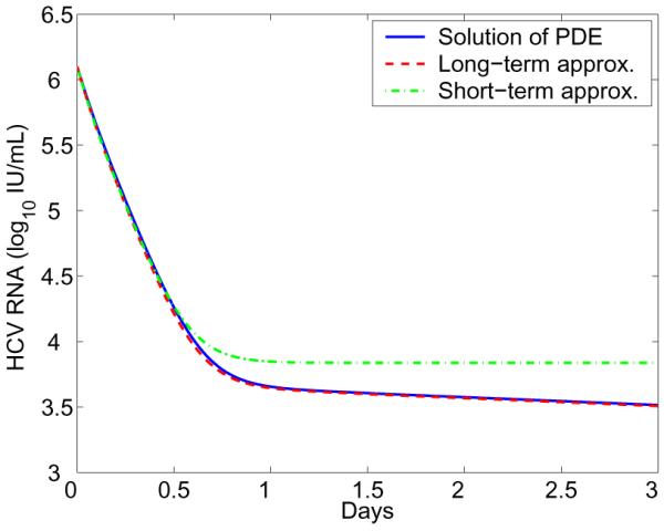
The blue solid line represents the numerical solution of the PDE model (Eq. 4). The green dash-dotted line represents the short-term approximation (Eq. 36). The red dashed line represents the long-term approximation (Eq. 38). Parameter values are chosen from the estimates in [25]: s = 1.3 × 10⁵ cells/mL, d = 0.01 day⁻¹, β = 5 × 10⁻⁸ mL day⁻¹ virion⁻¹, δ = 0.14 day⁻¹, ∊_α = 0.992, α = 40 day⁻¹, ∊_s = 0.56, ρ = 8.18 day⁻¹, k = 4.94, μ = 1 day⁻¹, and c = 22.3 day⁻¹.

5 Other models

In the above model (Eq. 4), we assumed that intracellular viral RNA is produced at a rate α(a) or constant α in deriving model approximations. This is a very simple assumption about RNA production within an infected cell. Further, when all new infections are neglected during therapy the intracellular RNA level is predicted to converge to a non-zero steady-state solution A/B (see Eq. 32). This may not be realistic under effective therapy since all viral RNA can be eliminated with long-term treatment in in vitro replicon systems [34]. We modify the equation of R(a, t) by introducing a new term, e^−γt, which represents the decay of replication templates such as negative strand HCV RNA after treatment initiation at t = 0. Assuming that all rates are constant, we obtain the R(a, t) equation

$$\frac{\partial }{\partial t}R(a,t)+\frac{\partial }{\partial a}R(a,t)=(1-{∊}_{\alpha })\alpha e^{-\gamma t}-\left[\right(1-{∊}_s)\rho +\kappa \mu ]R(a,t),$$ (39)

with the initial condition

$$R(a,0)=\stackrel{‒}{R}\left(a\right)=\frac{\alpha }{\rho +\mu }+(1-\frac{\alpha }{\rho +\mu })e^{-(\rho +\mu )a}.$$

We can also obtain the long-term approximation by neglecting all new infections under therapy. When a ≥ t, the characteristic curves, t−a = constant, can be described by the parametric equation t = τ, a = τ + a₀. Along the characteristic curves, we have

$$\frac{\mathit{dR}\left(a\right(\tau ),t(\tau \left)\right)}{d\tau }=(1-{∊}_{\alpha })\alpha e^{-\gamma t\left(\tau \right)}-\left[\right(1-{∊}_s)\rho +\kappa \mu ]R\left(a\right(\tau ),t(\tau \left)\right).$$

Using A = (1 − ∊_α)α and B = (1 − ∊_s)ρ + κμ, we have

$$\frac{\mathit{dR}}{d\tau }={\mathit{Ae}}^{-\gamma \tau }-\mathit{BR}.$$ (40)

Integrating τ from 0 to t, we have

$$\begin{array}{cc}\hfill R(a,t)& =R(a_0,0)e^{-\mathit{Bt}}+e^{-\mathit{Bt}}{\int }_0^t{e}^{\mathit{Bu}}{\mathit{Ae}}^{-\gamma u}\mathit{du}\hfill \\ \hfill & =\frac{A}{B-\gamma }{e}^{-\gamma t}+\left[\stackrel{‒}{R}\right(a-t)-\frac{A}{B-\gamma }]e^{-\mathit{Bt}},\text{for}a\ge t.\hfill \end{array}$$ (41)

The virus equation in the model where all new infections under therapy are ignored becomes

$$\frac{d}{\mathit{dt}}V\left(t\right)=(1-{∊}_s)\rho {\int }_t^{\infty }R(a,t)I(a,t)\mathit{da}-\mathit{cV}\left(t\right).$$ (42)

Using R(a, t) in Eq. (41) and $I(a,t)=\stackrel{‒}{I}(a-t)e^{-\delta t}=\beta \stackrel{‒}{V}\stackrel{‒}{T}{e}^{-\delta a}$ for a ≥ t, we calculate the integral

$$\begin{array}{cc}\hfill & {\int }_t^{\infty }R(a,t)I(a,t)\mathit{da}={\int }_t^{\infty }\left\{\frac{A}{B-\gamma }{e}^{-\gamma t}+\left[\stackrel{‒}{R}\right(a-t)-\frac{A}{B-\gamma }]e^{-\mathit{Bt}}\right\}\beta \stackrel{‒}{V}\stackrel{‒}{T}{e}^{-\delta a}\mathit{da}\hfill \\ \hfill & =\beta \stackrel{‒}{V}\stackrel{‒}{T}{\int }_t^{\infty }\left\{\frac{A}{B-\gamma }{e}^{-\gamma t}+[\frac{\alpha }{\rho +\mu }+(1-\frac{\alpha }{\rho +\mu })e^{-(\rho +\mu )(a-t)}-\frac{A}{B-\gamma }]e^{-\mathit{Bt}}\right\}{e}^{-\delta a}\mathit{da}\hfill \\ \hfill & =\beta \stackrel{‒}{V}\stackrel{‒}{T}\left\{\frac{A}{(B-\gamma )\delta }{e}^{-(\delta +\gamma )t}+[\frac{\alpha +\delta }{\delta (\rho +\mu +\delta }-\frac{A}{(B-\gamma )\delta }]e^{-(B+\delta )t}\right\}.\hfill \end{array}$$

Using

$$N=\frac{\rho (\alpha +\delta )}{\delta (\rho +\mu +\delta )}\text{and}\beta \stackrel{‒}{V}\stackrel{‒}{T}=\frac{c\stackrel{‒}{V}}{N},$$

we have

$${\int }_t^{\infty }R(a,t)I(a,t)\mathit{da}=\frac{c\stackrel{‒}{V}}{N}\left\{\frac{A}{(B-\gamma )\delta }{e}^{-(\delta +\gamma )t}+[\frac{N}{\rho }-\frac{A}{(B-\gamma )\delta }]e^{-(B+\delta )t}\right\}.$$

Plugging the above integral into the virus equation (42) and solving for V (t), we obtain

$$\begin{array}{cc}\hfill \frac{V\left(t\right)}{V_0}& =e^{-\mathit{ct}}+(1-{∊}_s)\frac{c\rho }{N}\{\frac{A}{(B-\gamma )\delta (\delta +\gamma -c)}(e^{-\mathit{ct}}-e^{-(\delta +\gamma )t})\phantom{\}}\hfill \\ \hfill & \phantom{\{}+\frac{1}{B+\delta -c}\left(\frac{N}{\rho }-\frac{A}{(B-\gamma )\delta }\right)(e^{-\mathit{ct}}-e^{-(B+\delta )t})\}.\hfill \end{array}$$ (43)

This is the long-term approximation to the viral load decline after therapy initiation, predicted by Eq. (4) in which the R(a, t) equation is replaced by (39).

We compare the long-term approximation (Eq. 43) with the solution of the corresponding PDE model. Numerical result shows that with realistic parameter values characteristic of potent therapy the approximation agrees very well with the PDE model solution (Figure 2). This approximation was used to fit the viral load data from eight HCV patients treated with a protease inhibitor danoprevir [25]. The effectiveness of danoprevir in blocking intracellular viral production, enhancing viral degradation, and inhibiting viral assembly or secretion was estimated on the basis of the best fits [25].

Figure 2. Comparison of the PDE model including an exponentially decreasing term with its approximation.

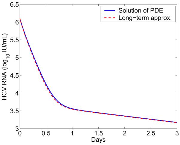
The blue solid line represents the numerical solution of Eq. (4) with the R equation replaced by Eq. (39). The red dashed line represents the long-term approximation (Eq. 43). The parameter γ is chosen to be γ = 0.28 day⁻¹ [25]. The other parameters are the same as those in Figure 1.

There are other possible ways to model intracellular viral dynamics within an infected cell. Because positive strand HCV RNA is made from a “replication complex” containing both HCV proteins and negative strand RNA [5], we can assume that the production rate of positive strand RNA is a function of both the level of negative strand RNA and the level of HCV proteins, which in turn should be proportional to R as viral RNA acts as the messenger RNA needed to produce viral proteins. Because negative strand RNA is synthesized from positive strand RNA [5], the level of negative strand RNA also could be proportional to R. Thus, another possible model that considers HCV proteins and negative strand RNA can be described by the following equation

$$\frac{\partial }{\partial t}R(a,t)+\frac{\partial }{\partial a}R(a,t)=(1-{∊}_{\alpha })\alpha R^2(a,t)-\left[\right(1-{∊}_s)\rho +\kappa \mu ]R(a,t).$$ (44)

The boundary condition is R(0, t) = 1 and the initial condition is $R(a,0)=\stackrel{‒}{R}\left(a\right)$, where $\stackrel{‒}{R}\left(a\right)$ is the steady-state age distribution of R(a, t) before therapy, given by

$$\stackrel{‒}{R}\left(a\right)=\frac{\rho +\mu }{\alpha +(\rho +\mu -\alpha )e^{(\rho +\mu )a}}.$$ (45)

Note that ρ + μ should be greater than or equal to α in order to avoid the explosion of α.

Using the method of characteristics, we obtain a complete solution for R(a, t)

$$R(a,t)=\{\begin{array}{cc}\frac{B}{A+(B-A)e^{\mathit{Ba}}}\hfill & \text{for}a<t,\hfill \\ \frac{B\stackrel{‒}{R}(a-t)}{A\stackrel{‒}{R}(a-t)+[B-A\stackrel{‒}{R}(a-t\left)\right]e^{\mathit{Bt}}}\hfill & \text{for}a\ge t,\hfill \end{array}\phantom{\}}$$ (46)

where A = (1 − ∊_α)α, B = (1 − ∊_s)ρ + κμ, and $\stackrel{‒}{R}\left(a\right)$ is given in (45).

In this case, even with the assumption of a constant level of infected cells or no new infections after treatment initiation, we cannot obtain an analytical approximation to the viral load decline like Eq. (36), (38), or (43). Numerical simulation in Figure 3 suggests that the viral load predicted by the model undergoes an initial minor increase, followed by a rapid decrease. Such transient initial increases in HCV viral load following initiation of therapy were reported by Hsu et al. [35] but interpreted by Guedj et al. [36] as possibly arising in patients whose pre-therapy viral load was increasing rather than being at steady state. This new model provides an alternative explanation.

Figure 3. Viral load change predicted by the model including a nonlinear RNA production rate (Eq. 44).

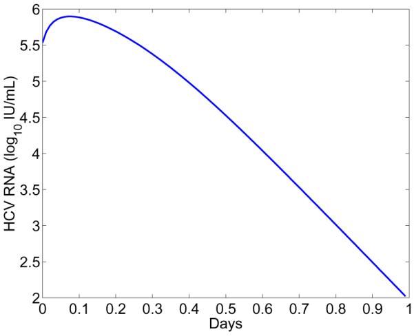
Parameter values are: ∊_α = 0.94, ∊_s = 0.5, α = 14 day⁻¹ mL RNA⁻¹, ρ = 13 day⁻¹. The other parameters are the same as those in Figure 1.

6 Effect of therapy on dynamics

Since Eq. (43) provides an excellent approximation to the solution of the multiscale PDE model, we examine it in more detail to gain insights into the effect of therapy on viral load decline after treatment initiation. There are three exponential terms in the approximation, e^−ct, e^−(B+δ)t, and e^−(γ+δ)t, where B = (1 − ∊_s)ρ + κμ. The first exponential term represents the viral clearance. The second term represents the loss of intracellular viral RNA by export and degradation as well as elimination of infected cells. The third term represents a combination of the reduction in intracellular viral RNA production and the elimination of infected cells. Three exponential terms suggest that a triphasic viral decline may be observed on a logarithmic scale after treatment initiation, compared with the biphasic viral decline predicted by the basic viral dynamic model [17]. However, this is not always the case. Whether a triphasic vial load decline can be observed also depends on the coefficients before the exponential terms. In fact, Eq. (43) can be rewritten as

$$\frac{V\left(t\right)}{V_0}=C_1{e}^{-\mathit{ct}}+C_2{e}^{-(B+\delta )t}+C_3{e}^{-(\gamma +\delta )t},$$

where

$$C_1=1-(1-{∊}_s)\frac{c\rho }{N}\left[\frac{A}{(B-\gamma )\delta (c-\delta -\gamma )}+\frac{1}{c-B-\delta }\left(\frac{N}{\rho }-\frac{A}{(B-\gamma )\delta }\right)\right]$$

$$C_2=(1-{∊}_s)\frac{c\rho }{N}\cdot \frac{1}{c-B-\delta }\left(\frac{N}{\rho }-\frac{A}{(B-\gamma )\delta }\right),$$

$$C_3=(1-{∊}_s)\frac{c\rho }{N}\cdot \frac{A}{(B-\gamma )\delta (c-\delta -\gamma )}.$$

The duration of the first-phase viral decline, denoted by D₁, is the time at which two curves log₁₀(C₁e^−ct) and log₁₀[C₂e^−(B+δ)t] intersect. Thus, we have

$$D_1=\frac{\ln \left(\frac{C_1}{C_2}\right)}{c-(B+\delta )}.$$

Similarly, we have the duration of the second-phase viral decline

$$D_2=\frac{\ln \left(\frac{C_2}{C_3}\right)}{B-\gamma }.$$

If ∊_s is close to 1, then C₁ >> C₂ and there is a visible first-phase viral decline with slope c. If ∊_α is close to 1, then A = (1 − ∊_α)α is very small. As a consequence, C₂ >> C₃ and there is a visible second-phase viral decline with slope B + δ. Numerical simulations in Figure 4 confirm these theoretical predictions. When therapy significantly blocks both intracellular viral production (∊_α = 0.99) and secretion (∊_s = 0.99), the viral load decline has three phases (blue solid line), with slopes c, (1 − ∊_s)ρ + κμ + δ, and γ + δ, respectively. As ∊_α decreases, the duration of the first-phase viral decline with slope c declines and the second phase with slope (1 − ∊_s)ρ + κμ + δ disappears (blue dash-dotted and blue dashed). When ∊_s = 0.01, the first-phase viral decline with slope c is not visible (red dotted). These results may explain why the estimate of the viral clearance rate c under therapy with DAAs such as the NS5A inhibitor daclatasvir is significantly higher than the estimate of c under traditional IFN-based therapy [24].

Figure 4. Effect of therapy on viral load change.

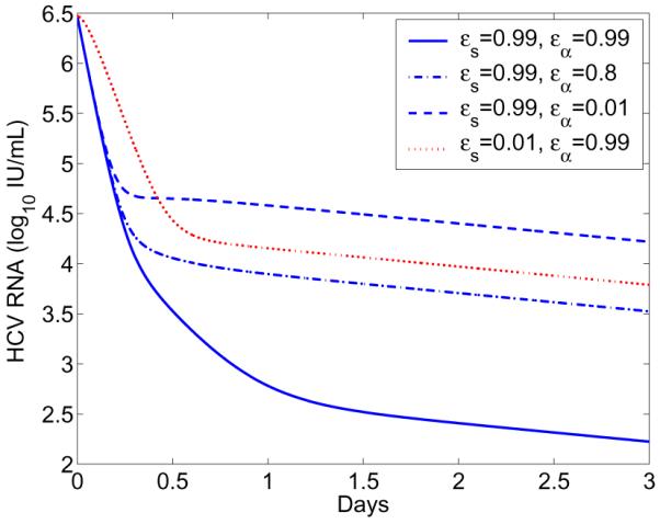
The long-term approximation (Eq. 43) was plotted with different combinations of drug efficacies ∊_s and ∊_α. The other parameter values are the same as those in Figure 1.

7 Conclusions

Treatment with direct-acting antiviral agents has greatly increased the cure rate in hepatitis C patients when used in combination with traditional IFN-based therapy. The dynamics of HCV under DAA therapy has started to be explored [23–25, 37–43] but much remains to be done [16, 44–46]. A viral dynamic model that does not consider intracellular viral dynamics may not be optimal in studying the dynamics in patients treated with DAAs, since these agents directly interfere with various steps in the HCV life cycle. In this paper, we analyzed multiscale models that include both intracellular viral RNA replication and extracellular viral infection dynamics.

We calculated the steady states of one such multiscale model and performed a thorough local stability analysis of the steady states. Specifically, the infection-free steady state is locally asymptotically stable when the basic reproductive ratio is less than 1 and the infected steady state is locally asymptotically stable whenever it exists. Under certain assumptions, we also obtained analytical approximations to the solution of the multiscale model. One approximation assuming no new infections during therapy agrees very well with the prediction of the multiscale model. This approximation has been used to fit patient data treated with DAAs and estimate parameter values such as the viral clearance rate and the treatment effectiveness.

Multiscale models allow us to explicitly consider the possible effects of DAAs on intracellular viral RNA production, degradation, and assembly and secretion as virus into the circulation. We showed that if therapy can significantly block viral secretion, then the first-phase viral load decline reflects the rate of viral clearance in plasma. If therapy can also block intracellular viral production significantly, then there is a visible second-phase viral decline, which reflects the loss of intracellular viral RNA. A third phase reflects the rate of loss of HCV replication complexes or negative strand RNA and the rate of infected cell death. Combined with experimental data, these results can be used to explore the possible mechanisms of action of DAAs against HCV.

• -We study hepatitis C virus dynamics using a multiscale age-structured model
• -The model includes intracellular RNA replication and extracellular viral infection
• -Stability analysis of the steady states is performed
• -Approximations of the viral decline are derived and compared with the full model
• -We discuss other ways to incorporate intracellular viral dynamics into the model

References

- 1.World Health Organization Hepatitis C. Fact sheet No. 164. Revised June 2011. http://www.who.int/mediacentre/factsheets/fs164/en/index.html.
- 2.Foster GR. Past, present, and future hepatitis C treatments. Semin Liver Dis. 2004;24(Suppl 2):97–104. doi: 10.1055/s-2004-832934. [DOI] [PubMed] [Google Scholar]
- 3.Fusco DN, Chung RT. Novel therapies for hepatitis C: insights from the structure of the virus. Annu Rev Med. 2012;63:373–87. doi: 10.1146/annurev-med-042010-085715. [DOI] [PubMed] [Google Scholar]
- 4.Hoofnagle JH. A step forward in therapy for hepatitis C. N Engl J Med. 2009;360:1899–901. doi: 10.1056/NEJMe0901869. [DOI] [PubMed] [Google Scholar]
- 5.Pawlotsky JM, Chevaliez S, McHutchison JG. The hepatitis C virus life cycle as a target for new antiviral therapies. Gastroenterology. 2007;132:1979–98. doi: 10.1053/j.gastro.2007.03.116. [DOI] [PubMed] [Google Scholar]
- 6.Rice CM. New insights into HCV replication: potential antiviral targets. Top Antivir Med. 2011;19:117–20. [PMC free article] [PubMed] [Google Scholar]
- 7.Poordad F, Dieterich D. Treating hepatitis C: current standard of care and emerging direct-acting antiviral agents. J Viral Hepat. 2012;19:449–64. doi: 10.1111/j.1365-2893.2012.01617.x. [DOI] [PubMed] [Google Scholar]
- 8.Sarrazin C, Hezode C, Zeuzem S, Pawlotsky JM. Antiviral strategies in hepatitis C virus infection. J Hepatol. 2012;56(Suppl 1):S88–100. doi: 10.1016/S0168-8278(12)60010-5. [DOI] [PubMed] [Google Scholar]
- 9.Gao M, Nettles RE, Belema M, Snyder LB, Nguyen VN, Fridell RA, Serrano-Wu MH, Langley DR, Sun JH, O'Boyle n., D. R., Lemm JA, Wang C, Knipe JO, Chien C, Colonno RJ, Grasela DM, Meanwell NA, Hamann LG. Chemical genetics strategy identifies an HCV NS5A inhibitor with a potent clinical effect. Nature. 2010;465:96–100. doi: 10.1038/nature08960. [DOI] [PMC free article] [PubMed] [Google Scholar]
- 10.Gane EJ, Rouzier R, Stedman C, Wiercinska-Drapalo A, Horban A, Chang L, Zhang Y, Sampeur P, Najera I, Smith P, Shulman NS, Tran JQ. Antiviral activity, safety, and pharmacokinetics of danoprevir/ritonavir plus PEG-IFN alpha-2a/RBV in hepatitis, C patients. J Hepatol. 2011;55:972–9. doi: 10.1016/j.jhep.2011.01.046. [DOI] [PubMed] [Google Scholar]
- 11.Forestier N, Larrey D, Marcellin P, Guyader D, Patat A, Rouzier R, Smith PF, Qin X, Lim S, Bradford W, Porter S, Seiwert SD, Zeuzem S. Antiviral activity of danoprevir (ITMN-191/RG7227) in combination with pegylated interferon alpha-2a and ribavirin in patients with hepatitis C. J Infect Dis. 2011;204:601–8. doi: 10.1093/infdis/jir315. [DOI] [PubMed] [Google Scholar]
- 12.Ciesek S, von Hahn T, Manns MP. Second-wave protease inhibitors: choosing an heir. Clin Liver Dis. 2011;15:597–609. doi: 10.1016/j.cld.2011.05.014. [DOI] [PubMed] [Google Scholar]
- 13.Schaefer EA, Chung RT. Anti-hepatitis C virus drugs in development. Gastroenterology. 2012;142:1340–1350. e1. doi: 10.1053/j.gastro.2012.02.015. [DOI] [PubMed] [Google Scholar]
- 14.Herrmann E, Neumann AU, Schmidt JM, Zeuzem S. Hepatitis C virus kinetics. Antivir Ther. 2000;5:85–90. [PubMed] [Google Scholar]
- 15.Guedj J, Rong L, Dahari H, Perelson AS. A perspective on modelling hepatitis C virus infection. J Viral Hepat. 2010;17:825–33. doi: 10.1111/j.1365-2893.2010.01348.x. [DOI] [PMC free article] [PubMed] [Google Scholar]
- 16.Rong L, Perelson AS. Treatment of hepatitis C virus infection with interferon and small molecule direct antivirals: viral kinetics and modeling. Crit Rev Immunol. 2010;30:131–48. doi: 10.1615/critrevimmunol.v30.i2.30. [DOI] [PMC free article] [PubMed] [Google Scholar]
- 17.Neumann AU, Lam NP, Dahari H, Gretch DR, Wiley TE, Layden TJ, Perelson AS. Hepatitis C viral dynamics in vivo and the antiviral efficacy of interferon-alpha therapy. Science. 1998;282:103–7. doi: 10.1126/science.282.5386.103. [DOI] [PubMed] [Google Scholar]
- 18.Lau JY, Tam RC, Liang TJ, Hong Z. Mechanism of action of ribavirin in the combination treatment of chronic HCV infection. Hepatology. 2002;35:1002–9. doi: 10.1053/jhep.2002.32672. [DOI] [PubMed] [Google Scholar]
- 19.Pawlotsky JM, Dahari H, Neumann AU, Hezode C, Germanidis G, Lonjon I, Cast-era L, Dhumeaux D. Antiviral action of ribavirin in chronic hepatitis C. Gastroenterology. 2004;126:703–14. doi: 10.1053/j.gastro.2003.12.002. [DOI] [PubMed] [Google Scholar]
- 20.Herrmann E, Lee J, Marinos G, Modi M, Zeuzem S. Effect of ribavirin on hepatitis C viral kinetics in patients treated with pegylated interferon. Hepatology. 2003;37:1351–8. doi: 10.1053/jhep.2003.50218. [DOI] [PubMed] [Google Scholar]
- 21.Dixit NM, Layden-Almer JE, Layden TJ, Perelson AS. Modelling how ribavirin improves interferon response rates in hepatitis C virus infection. Nature. 2004;432:922–4. doi: 10.1038/nature03153. [DOI] [PubMed] [Google Scholar]
- 22.Layden-Almer JE, Ribeiro RM, Wiley T, Perelson AS, Layden TJ. Viral dynamics and response differences in HCV-infected african american and white patients treated with IFN and ribavirin. Hepatology. 2003;37:1343–50. doi: 10.1053/jhep.2003.50217. [DOI] [PubMed] [Google Scholar]
- 23.Guedj J, Neumann AU. Understanding hepatitis C viral dynamics with direct-acting due to the interplay between intracellular replication and cellular infection dynamics. J Theor Biol. 2010;267:330–40. doi: 10.1016/j.jtbi.2010.08.036. [DOI] [PubMed] [Google Scholar]
- 24.Guedj J, Dahari H, Rong L, Sansone ND, Nettles RE, Cotler SJ, Layden TJ, Uprichard SL, Perelson AS. Modeling shows that the NS5A inhibitor daclatasvir has two modes of action and yields a shorter estimate of the hepatitis C virus half-life. Proc Natl Acad Sci U S A. 2013;110:3991–6. doi: 10.1073/pnas.1203110110. [DOI] [PMC free article] [PubMed] [Google Scholar]
- 25.Rong L, Guedj J, Dahari H, Coffield DJ, Levi M, Smith P, Perelson AS. Analysis of hepatitis C virus decline during treatment with the protease inhibitor danoprevir using a multiscale model. PLoS Comput Biol. 2013;9:e1002959. doi: 10.1371/journal.pcbi.1002959. [DOI] [PMC free article] [PubMed] [Google Scholar]
- 26.Nelson PW, Gilchrist MA, Coombs D, Hyman JM, Perelson AS. An age-structured model of HIV infection that allows for variations in the production rate of viral particles and the death rate of productively infected cells. Math Biosci Eng. 2004;1:267–88. doi: 10.3934/mbe.2004.1.267. [DOI] [PubMed] [Google Scholar]
- 27.Rong L, Feng Z, Perelson AS. Mathematical modeling of HIV-1 infection and drug therapy. In: Mondaini RP, Pardalos PM, editors. Mathematical Modeling of Biosystems. Springer-Verlag; 2008. pp. 87–131. [Google Scholar]
- 28.Gripenberg G, Londen SO, Staffans O. Volterra Integral and Functional Equations. Cambridge University Press; New York: 1990. [Google Scholar]
- 29.Thieme HR. Semiflows generated by Lipschitz perturbations of non-densely defined operators. Differential Integral Equations. 1990;3:1035–66. [Google Scholar]
- 30.Webb GF. Theory of Nonlinear Age-dependent Population Dynamics. CRC Press; 1985. [Google Scholar]
- 31.Thieme HR, Castillo-Chavez C. How may infection-age-dependent infectivity affect the dynamics of HIV/AIDS? SIAM J Appl Math. 1993;53:1447–79. [Google Scholar]
- 32.Feng Z, Iannelli M, Milner F. A two-strain TB model with age-structure. SIAM J Appl Math. 2002;62:1634–56. [Google Scholar]
- 33.Rong L, Feng Z, Perelson AS. Mathematical analysis of age-structured HIV-1 dynamics with combination antiretroviral therapy. SIAM J Appl Math. 2007;67:731–56. [Google Scholar]
- 34.Lin K, Kwong AD, Lin C. Combination of a hepatitis C virus NS3-NS4A protease inhibitor and alpha interferon synergistically inhibits viral RNA replication and facilitates viral RNA clearance in replicon cells. Antimicrob Agents Chemother. 2004;48:4784–92. doi: 10.1128/AAC.48.12.4784-4792.2004. [DOI] [PMC free article] [PubMed] [Google Scholar]
- 35.Hsu CS, Hsu SJ, Chen HC, Tseng TC, Liu CH, Niu WF, Jeng J, Liu CJ, Lai MY, Chen PJ, Kao JH, Chen DS. Association of IL28B gene variations with mathematical modeling of viral kinetics in chronic hepatitis C patients with IFN plus ribavirin therapy. Proc Natl Acad Sci U S A. 2011;108:3719–24. doi: 10.1073/pnas.1100349108. [DOI] [PMC free article] [PubMed] [Google Scholar]
- 36.Guedj J, Dahari H, Perelson AS. Understanding the nature of early HCV RNA blips and the use of mathematical modeling of viral kinetics during IFN-based therapy. Proc Natl Acad Sci U S A. 2011;108:E302. doi: 10.1073/pnas.1104149108. [DOI] [PMC free article] [PubMed] [Google Scholar]
- 37.Rong L, Dahari H, Ribeiro RM, Perelson AS. Rapid emergence of protease inhibitor resistance in hepatitis C virus. Sci Transl Med. 2010;2:30–32. doi: 10.1126/scitranslmed.3000544. [DOI] [PMC free article] [PubMed] [Google Scholar]
- 38.Rong L, Ribeiro RM, Perelson AS. Modeling quasispecies and drug resistance in hepatitis C patients treated with a protease inhibitor. Bull Math Biol. 2012;74:1789–817. doi: 10.1007/s11538-012-9736-y. [DOI] [PMC free article] [PubMed] [Google Scholar]
- 39.Guedj J, Perelson AS. Second-phase hepatitis C virus RNA decline during telaprevir-based therapy increases with drug effectiveness: implications for treatment duration. Hepatology. 2011;53:1801–8. doi: 10.1002/hep.24272. [DOI] [PMC free article] [PubMed] [Google Scholar]
- 40.Guedj J, Dahari H, Pohl RT, Ferenci P, Perelson AS. Understanding silibinin's modes of action against HCV using viral kinetic modeling. J Hepatol. 2012;56:1019–24. doi: 10.1016/j.jhep.2011.12.012. [DOI] [PMC free article] [PubMed] [Google Scholar]
- 41.Guedj J, Dahari H, Shudo E, Smith P, Perelson AS. Hepatitis C viral kinetics with the nucleoside polymerase inhibitor mericitabine (RG7128) Hepatology. 2012;55:1030–7. doi: 10.1002/hep.24788. [DOI] [PMC free article] [PubMed] [Google Scholar]
- 42.Adiwijaya BS, Herrmann E, Hare B, Kieffer T, Lin C, Kwong AD, Garg V, Randle JC, Sarrazin C, Zeuzem S, Caron PR. A multi-variant, viral dynamic model of genotype 1 HCV to assess the in vivo evolution of protease-inhibitor resistant variants. PLoS Comput Biol. 2010;6:e1000745. doi: 10.1371/journal.pcbi.1000745. [DOI] [PMC free article] [PubMed] [Google Scholar]
- 43.Adiwijaya BS, Kieffer TL, Henshaw J, Eisenhauer K, Kimko H, Alam JJ, Kauffman RS, Garg V. A viral dynamic model for treatment regimens with direct-acting antivirals for chronic hepatitis C infection. PLoS Comput Biol. 2012;8:e1002339. doi: 10.1371/journal.pcbi.1002339. [DOI] [PMC free article] [PubMed] [Google Scholar]
- 44.Dahari H, Guedj J, Perelson AS, Layden TJ. Hepatitis C viral kinetics in the era of direct acting antiviral agents and IL28B. Curr Hepat Rep. 2011;10:214–227. doi: 10.1007/s11901-011-0101-7. [DOI] [PMC free article] [PubMed] [Google Scholar]
- 45.Chaterjee A, Guedj J, Perelson AS. Mathematical modeling of HCV infection: what can it teach us in the era of direct antiviral agents? Antivir Ther. 2012;17:1171–82. doi: 10.3851/IMP2428. [DOI] [PMC free article] [PubMed] [Google Scholar]
- 46.Chaterjee A, Smith PF, Perelson AS. Hepatitis C viral kinetics: the past, present and future. Clin Liver Dis. 2013;17:13–26. doi: 10.1016/j.cld.2012.09.003. [DOI] [PMC free article] [PubMed] [Google Scholar]