Identifying fMRI Model Violations with Lagrange Multiplier Tests

Abstract

The standard modeling framework in Functional Magnetic Resonance Imaging (fMRI) is predicated on assumptions of linearity, time invariance and stationarity. These assumptions are rarely checked because doing so requires specialised software, although failure to do so can lead to bias and mistaken inference. Identifying model violations is an essential but largely neglected step in standard fMRI data analysis.

Using Lagrange Multiplier testing methods we have developed simple and efficient procedures for detecting model violations such as non-linearity, non-stationarity and validity of the common Double Gamma specification for hemodynamic response. These procedures are computationally cheap and can easily be added to a conventional analysis.

The test statistic is calculated at each voxel and displayed as a spatial anomaly map which shows regions where a model is violated.

The methodology is illustrated with a large number of real data examples.

I. Introduction

A standard feature of statistical modeling [1], [2], [3] is to carry out diagnostic tests of the assumptions behind the model. But this kind of model criticism has not become commonplace in fMRI data analysis. A consequence is that model violations can lead to wrong conclusions and failure to find sought after effects.

It would be useful to be able to readily determine whether standard models are adequate for the data at hand or whether more complicated methods are required, without a lot of additional modeling or computation. This paper describes tools we have developed for such assessments.

The linear, time-invariant (LTI) assumption of fMRI analysis is an approximation of underlying signal behaviour. The assumption is reasonable to first order [4] for most, but not all fMRI data. Temporal non-linear and non-stationary effects can be observed [5], [6], [7], [8] as the BOLD (Blood Oxygen Level Dependent) response varies spatially across the brain and temporally between scans [9].

The Double Gamma is a popular model for the Hemodynamic Response Function (HRF), which underpins conventional fMRI analyses. But its validity on a particular data volume is rarely checked.

Previous attempts at diagnosing model violation in fMRI have offered mostly exploratory or empirical indications of model anomalies [10]. Among those methods, test statistics have been suggested for investigating noise characteristics such as measuring the overall normality, independence or auto-regression within data residuals [11], [12]. Other important sources of model violation within both fMRI signal and noise have been only loosely characterised [13].

A quantitative approach to examining model violations would be based upon methods such as Likelihood Ratio Tests (LRT), which require model fitting under the null and the alternative hypotheses. They are usually computationally expensive and typically involve considerable algorithmic and software development; perhaps for these reasons they are rarely done.

Our approach to model diagnostic tests is based on the Lagrange multiplier (LM) testing procedure. Preliminary versions of this approach have appeared in two abstracts [14], [15]. The LM method (also known as the score testing method) has a long history in statistics [16] and has found widespread application in econometrics [17], [18]. The crucial feature of the LM approach is that it only requires model fitting under the null hypothesis. This leads to cheap computational procedures involving linear regression that can be easily added to a standard analysis. The result is a measure of model violation at each voxel which, when plotted spatially, we call an LM-anomaly map. Each possible model violation tested generates an associated LM-anomaly map.

If an LM-anomaly map detects violation within an fMRI volume for a particular model, an appropriate replacement model must be specified to ensure results from subsequent analyses can be trusted. Such an alternative model is contained within the structure of the LM-anomaly test.

The remainder of this paper is organised as follows.

In Section 2 we reiterate the motivation for model diagnostic testing. In Section 3 we review the theory of LM tests and end with a summary of the procedure. In Section 4 several tests of common fMRI model inadequacies are developed: a Time-Varying HRF, the Double Gamma HRF fit and Non-Linear HRF. In Section 5 these are illustrated on a large amount of fMRI data. Discussion and conclusions are offered in Sections 6 and 7 respectively.

Notation and Acronyms

MLE = maximum likelihood estimator; LM = Lagrange multiplier; AR = autoregressive or autoregression; θ̃ is a constrained MLE; θ̂ is an unconstrained MLE; ${\tilde{L}}_{\pi }=\frac{\partial L}{\partial \tilde{\pi }}$; superscript H denotes Hermitian transpose i.e. complex conjugate transpose; (k) or subscript [k] indicates a frequency domain signal.

II. Model Criticism Background

The notion that statistical models can be wrong, indeed are always wrong¹ and that there is thus a need for a formal model criticism (followed if necessary by changes to the model) has a long history in statistics (see e.g. the first edition of [20]). Such methods now form a standard part of all modern statistical data analysis. But this practice has diffused slowly into applied fields such as fMRI and allied fields such as statistical signal processing and machine learning.

How then should one carry out a process of model criticism or develop model diagnostics? Two approaches have emerged. An exploratory or omnibus approach and a more formal approach. We now briefly discuss each.

The earliest model criticism or model diagnostic approaches involved analysis of residuals; for details see [20], [3] (and earlier editions) and the classic monograph [1], which continues to be important. The idea is simply that if the model is correct the residuals should show no patterns nor be related to any regressors of interest.

Additional model criticism methods have continued to be developed e.g. outlier methods [3]. Compelling examples of these methods have already been exhibited in fMRI e.g. [11], [12], [13]. However many of these approaches while very useful are more in the nature of exploratory methods.

The econometrics community has also thoroughly embraced the model criticism issue but tended towards a formal approach. Thus testing for model misspecification similarly has a long history there [21], and in particular Lagrange multiplier methods emerged [17], [22], [18] in the late 1970s as a versatile formal approach.

The formal approach has the advantage that, unlike the exploratory approach, the model violation of concern has to be explicitly formulated as an alternative hypothesis. It is thus more able to find particular kinds of violation than the omnibus exploratory methods. This formal approach then forms our point of departure.

III. Methods

Although exposés of LM theory exist [17], [22], [18], being couched in an econometric context they are not easily accessible; also we need to develop some aspects not dealt with in those works. Consequently we provide a self-contained development.

Suppose we have n-dimensional data Y distributed according to a likelihood, dependent on a p-dimensional parameter θ,

$$\text{log likelihood}=L(Y;\theta )=L(\theta )\text{for simplicity}.$$

L (θ) is twice differentiable.

Consider a general hypothesis, H₀ : g(θ) = 0 where g(θ) is an r-vector of differentiable functions. We introduce the constrained MLE, θ̃ and the unconstrained MLE, θ̂,

$$\tilde{\theta }=\text{arg}\underset{g(\theta )=0}{\text{max}}L(\theta )\widehat{\theta }=\text{arg max}L(\theta ),(\Rightarrow \frac{dL}{d\theta }=0)$$

A. Full Rank Theory

The LM test is developed via two Taylor series expansions applied to the log of the likelihood ratio: L(θ̂) − L(θ̃), namely,

$$L(\tilde{\theta })=L(\widehat{\theta })+\frac{1}{2}{(\tilde{\theta }-\widehat{\theta })}^T{L}_{{\theta }_{*}{\theta }_{*}}(\tilde{\theta }-\widehat{\theta })$$ (1)

$$0=\frac{dL}{d\widehat{\theta }}=\frac{dL}{d\tilde{\theta }}+L_{{\theta }_{*}{\theta }_{*}}(\widehat{\theta }-\tilde{\theta })$$ (2)

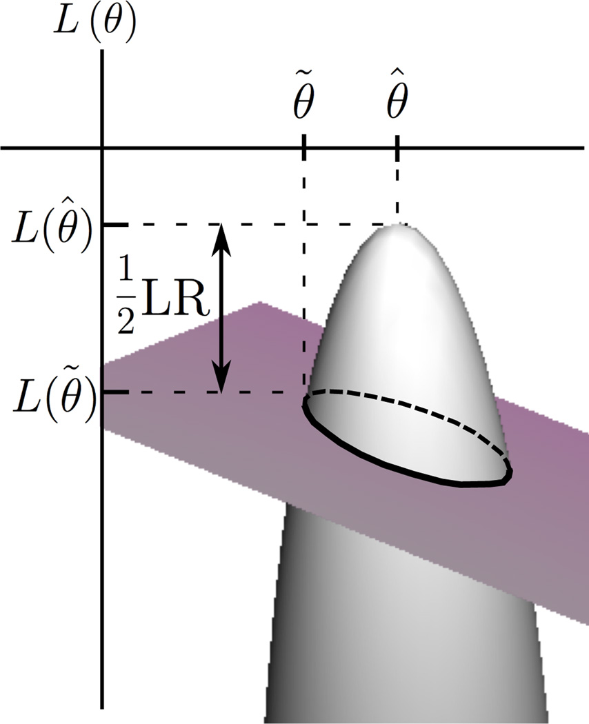
where (1) is the Taylor series approximation of L(θ̃) around θ̂, and (2) is the Taylor series expansion of $\frac{dL}{d\theta }$ around θ̃; also $L_{\theta \theta }=\frac{{\partial }^{2}L}{\partial \theta \partial \theta }$ and is evaluated at θ_* which denotes a value between θ̃ and θ̂. It is important to note that for large n (as is the case for fMRI) the log-likelihood function resembles a quadratic [23] with constant second-derivative (see Fig. 1). Therefore, although the actual value of L_θθ differs for θ̃ and θ̂ they asymptotically reach the same value so we can replace them both by θ_*. The latter Taylor series (2) gives

$$\widehat{\theta }-\tilde{\theta }=-L_{{\theta }_{*}{\theta }_{*}}^{-1}\frac{dL}{d\tilde{\theta }}\approx -L_{\tilde{\theta }\tilde{\theta }}^{-1}\frac{dL}{d\tilde{\theta }}$$

so substituting this in (1) gives an approximation to the likelihood ratio test statistic,

$$2(L(\widehat{\theta })-L(\tilde{\theta }))\approx -\frac{dL}{d{\tilde{\theta }}^T}{L}_{\tilde{\theta }\tilde{\theta }}^{-1}\frac{dL}{d\tilde{\theta }}$$ (3)

We now approximate L_θ̃θ̃ by the Fisher information, evaluated at θ̃,

$${ℐ}_{\theta \theta }=-E(L_{\theta \theta }){|}_{\theta =\tilde{\theta }}$$

which when substituted in (3) gives the LM statistic

$$V_{\tilde{\theta }}=\frac{dL}{d{\tilde{\theta }}^T}{\widetilde{ℐ}}_{\theta \theta }^{-1}\frac{dL}{d\tilde{\theta }}$$

The crucial feature of this test statistic is that to compute it we only need the constrained parameter estimator, i.e. we only need to fit the model under the null hypothesis [24]. This leads to very fast computation. We expect the LM test to have asymptotically a ${\chi }_{p-r}^2$ distribution [25], [16].

Figure 1.

Parameter spaces of the restricted and full models are the intersection curve and parabolic surface respectively. The Likelihood Ratio test gets LR from likelihoods at both maxima. The Lagrange Multiplier method approximates LR by calculating likelihood and curvature at only the restricted parameter estimate.

Result I

To test the hypothesis g (θ) = 0

1. Compute the constrained MLE θ̃.

2. Generate the gradient $\frac{dL}{d{\tilde{\theta }}^T}$ and the information matrix ℐ̃_θθ.

3. Compute the LM statistic $V_{\tilde{\theta }}=\frac{dL}{d{\tilde{\theta }}^T}{\widetilde{ℐ}}_{\theta \theta }^{-1}\frac{dL}{d\tilde{\theta }}$.

It has the asymptotic distribution ${\chi }_{p-r}^2$.

B. Sub-parameter Constraint

In many applications (including those here) the constraint or hypothesis is applied to only a subset of the parameters. So we partition θ = (π,ψ) and suppose the constraint is 0 = g(θ) = g(π). This leads to a reduction in the form of the LM test statistic.

To see what happens, we form the Lagrangian,

$$ℒ(\theta )=L(\theta )+g^T(\pi )\lambda$$

Then since π is constrained we have

$$\frac{\partial ℒ}{\partial \tilde{\pi }}=\frac{\partial L}{\partial \tilde{\pi }}+\frac{\partial g^T}{\partial \tilde{\pi }}\lambda =0$$

While ψ is unconstrained so,

$$\frac{\partial ℒ}{\partial \tilde{\psi }}=\frac{\partial L}{\partial \tilde{\psi }}=0$$

The LM statistic then becomes, (with ${\tilde{L}}_{\pi }=\frac{\partial L}{\partial \tilde{\pi }}$)

$$V_{\tilde{\theta }}=({\tilde{L}}_{\pi },0){\left(\begin{array}{ll}{\widetilde{ℐ}}_{\pi \pi }\hfill & {\widetilde{ℐ}}_{\pi \psi }\hfill \\ {\widetilde{ℐ}}_{\psi \pi }\hfill & {\widetilde{ℐ}}_{\psi \psi }\hfill \end{array}\right)}^{-1}\left(\begin{array}{c}{\tilde{L}}_{\pi }\\ 0\end{array}\right)$$ (4)

$$={\tilde{L}}_{\pi }^T{({\widetilde{ℐ}}_{\pi \pi }-{\widetilde{ℐ}}_{\pi \psi }{\widetilde{ℐ}}_{\psi \psi }^{-1}{\widetilde{ℐ}}_{\psi \pi })}^{-1}{\tilde{L}}_{\pi }$$ (5)

where we have used a well known formula for partitioned matrix inversion.

We summarise this in:

Result II

To test the sub-parameter hypothesis, g(π) = 0 where θ^T = (π^T, ψ^T),

1. Compute the constrained MLE, θ̃^T = (π̃^T, ψ̃^T)

2. Calculate the gradient, L̃_π and partitioned information matrix appearing in (4)

3. Compute the LM statistic given in (5).

C. Gaussian Likelihood with Sub-parameter Constraint

When the parameters are partitioned into mean and variance parameters we also get a simplification including a linear regressionlike structure. Suppose we partition,

$$\theta ={({\beta }^T,{\alpha }^T)}^T=(\text{system},\text{noise})$$

the log likelihood is then,

$$L(\theta )=-\frac{1}{2}{e}^T(\beta ){\mathrm{\Omega }}^{-1}(\alpha )e(\beta )-\frac{1}{2}\text{ln}|\mathrm{\Omega }(\alpha )|$$

where e = e (β) = Y − h(β), h(β) is the mean function and Ω (α) is the noise covariance. Assuming the errors are normally distributed as ε ~ N(0,Ω(α)), the constraint only involves the signal parameters affecting the mean. The partial derivatives of the log-likelihood function are then only dependent on β = (π^T, ψ^T)^T ; g (π) = 0. We then find,

$$\frac{\partial L}{\partial \pi }=Z^T{\mathrm{\Omega }}^{-1}e;Z^T=\frac{\partial h^T}{\partial \pi }\frac{\partial L}{\partial \psi }=0\leftrightarrow X^T{\mathrm{\Omega }}^{-1}\tilde{e}=0;X^T=\frac{\partial h^T}{\partial \psi }$$

So we can calculate the regression matrices under the null hypothesis condition,

$$\frac{\partial L}{\partial \tilde{\pi }}={\tilde{Z}}^T{\tilde{\mathrm{\Omega }}}^{-1}\tilde{e};{\tilde{Z}}^T=\frac{\partial h^T}{\partial \pi }{|}_{g(\pi )=0}$$ (6)

$$\frac{\partial L}{\partial \tilde{\psi }}=0\leftrightarrow {\tilde{X}}^T{\tilde{\mathrm{\Omega }}}^{-1}\tilde{e}=0;{\tilde{X}}^T=\frac{\partial h^T}{\partial \psi }{|}_{g(\pi )=0}$$ (7)

while

$$\left(\begin{array}{ll}{\widetilde{ℐ}}_{\pi \pi }\hfill & {\widetilde{ℐ}}_{\pi \psi }\hfill \\ {\widetilde{ℐ}}_{\psi \pi }\hfill & {\widetilde{ℐ}}_{\psi \psi }\hfill \end{array}\right)=\left(\begin{array}{ll}{\tilde{Z}}^T{\tilde{\mathrm{\Omega }}}^{-1}\tilde{Z}\hfill & {\tilde{Z}}^T{\tilde{\mathrm{\Omega }}}^{-1}\tilde{X}\hfill \\ {\tilde{X}}^T{\tilde{\mathrm{\Omega }}}^{-1}\tilde{Z}\hfill & {\tilde{X}}^T{\tilde{\mathrm{\Omega }}}^{-1}\tilde{X}\hfill \end{array}\right)$$ (8)

Then using partitioned matrix inversion (5) becomes V_θ̃ = V_β̃ so the LM test statistic is,

$$V_{\tilde{\beta }}=\frac{\partial L}{\partial {\tilde{\pi }}^T}{({\widetilde{ℐ}}_{\pi \pi }-{\widetilde{ℐ}}_{\pi \psi }{\widetilde{ℐ}}_{\psi \psi }^{-1}{\widetilde{ℐ}}_{\psi \pi })}^{-1}\frac{\partial T}{\partial \tilde{\pi }}={\tilde{e}}^T{\tilde{\mathrm{\Omega }}}^{-1}\tilde{Z}{({\tilde{Z}}^{T}U\tilde{Z})}^{-1}\tilde{Z}{\tilde{\mathrm{\Omega }}}^{-1}\tilde{e}$$ (9)

$$U={\tilde{\mathrm{\Omega }}}^{-1}-{\tilde{\mathrm{\Omega }}}^{-1}\tilde{X}{({\tilde{X}}^T{\tilde{\mathrm{\Omega }}}^{-1}\tilde{X})}^{-1}{\tilde{X}}^T{\tilde{\mathrm{\Omega }}}^{-1}$$ (10)

We summarise this in,

Result III

Suppose the likelihood has a Gaussian form with separate signal (β) and noise (α) parameters. To test the sub-signal-parameter hypothesis, g (π) = 0 where β^T = (π^T, ψ^T),

1. Compute the constrained MLEs, β̃^T and (π̃^T, ψ̃^T) and α̃.

2. Generate the error vector ẽ = Y − h (β̃) ; regression matrices Z̃, X̃ from (6),(7) and partitioned information matrix (8).

3. Compute the LM statistic given in (9),(10) or (11) below.

In many applications, the covariance matrix will be a Toeplitz matrix corresponding to a stationary noise. In that case the covariance matrix is approximately diagonalized by the discrete Fourier transform [26]. Then the LM statistic becomes,

$$V_{\tilde{\beta }}=(\sum \frac{{\tilde{e}}_{\left[k\right]}{\tilde{z}}_{\left[k\right]}^H}{{\tilde{F}}_{\left[k\right]}})Q^{-1}(\sum \frac{{\tilde{z}}_{\left[k\right]}{\tilde{e}}_{\left[k\right]}^H}{{\tilde{F}}_{\left[k\right]}})$$ (11)

$$Q=(\sum \frac{{\tilde{z}}_{\left[k\right]}{\tilde{z}}_{\left[k\right]}^H}{{\tilde{F}}_{\left[k\right]}})-(\sum \frac{{\tilde{z}}_{\left[k\right]}{\tilde{x}}_{\left[k\right]}^H}{{\tilde{F}}_{\left[k\right]}}){(\sum \frac{{\tilde{x}}_{\left[k\right]}{\tilde{x}}_{\left[k\right]}^H}{{\tilde{F}}_{\left[k\right]}})}^{-1}(\sum \frac{{\tilde{x}}_{\left[k\right]}{\tilde{z}}_{\left[k\right]}^H}{{\tilde{F}}_{\left[k\right]}})$$

where subscript [k] indicates a frequency domain signal and

$${\tilde{F}}_{\left[k\right]}=\tilde{F}\left(\frac{2\pi k}{T}\right)$$

is the fitted noise spectrum under the null hypothesis; T = dim (Y).

This frequency domain expression is important not only because it leads to cheap computation but also it enables us to understand intuitively what the LM-statistic is doing.

Firstly we factor the spectrum as ${\tilde{F}}_{\left[k\right]}={\varphi }_{\left[k\right]}{\varphi }_{\left[k\right]}^H$, e.g. if we have an AR(1) spectrum then ${\varphi }_{\left[k\right]}=\frac{\sigma }{1-\varphi e^{-j{\omega }_k}}$. Then the first bracket of the numerator in V_β̃ has the form ${\sum }_k\frac{{\tilde{e}}_{\left[k\right]}}{{\varphi }_{\left[k\right]}}\frac{{\tilde{z}}_{\left[k\right]}^H}{{\varphi }_{\left[k\right]}^H}$. Thus the numerator is a squared correlation between a filtered residual and a filtered synthetic regressor signal. This synthetic signal represents the potential presence of the anomaly. If the anomaly is present, then it will remain in the residual and so the correlation will be large. The Q matrix normalises the squared correlation, accounting for the effect of the regressor x̃_[k] and the noise.

D. Summary of Lagrange Multiplier Procedure

The steps to design a test for a particular model violation using the Lagrange Multiplier procedure are as follows:

1. Incorporate the anomaly of concern in a statistical model; e.g. y = h(π,ψ)+(noise), where ψ represents standard parameters; π represents the anomaly and vanishes if the anomaly is absent.

2. Fit the model under the null hypothesis g (π) = 0; i.e. fit y = h(π,ψ) + (noise) and thus generate a residual ẽ. Adjust the model fit to account for AR or other noise characteristics.

3. Calculate regression matrices $X=\frac{\partial h}{\partial \psi }$ and $Z=\frac{\partial h}{\partial \pi }$. X has size (T ×(p − r)), Z is (T × r) where T = dim(y), (p − r) = dim (ψ) and r = dim (π).

4. Evaluate the regression matrices under the null hypothesis as X̃ = X|_β=β̃,Z̃ = Z|_β=β̃. We call Z̃ the anomaly regression matrix.

5. F̃_[k] is the unbiased estimate of the noise spectrum under H₀.

6. Calculate the test statistic of (11) in the frequency domain.

The test is applied individually to each voxel time-series in an fMRI data volume. The resulting test statistics are plotted spatially as an LM-anomaly map. Applying a Bonferroni-corrected [27] threshold to the test statistic based upon the ${\chi }_{p-r}^2$ distribution and desired accuracy level gives a spatial LM-anomaly map showing the significant areas of model violation.

The anomaly regression matrix Z̃ emphasises the link between the LM procedure and the process of choosing explanatory variables to include in a regression analysis. The LM testing approach would equate to objectively selecting additional model regressors, rather than an heuristic choice based upon intuition.

E. What to do if a Model Violation Occurs

If model violation is detected, then the model being tested under the null hypothesis is invalid and a different model must be fitted. Since the LM test construction already requires specification of a model under the alternative hypothesis, this model is a natural candidate to be tested. Yet that requires fitting under the alternative and then construction of a likelihood ratio test; all of this needs specialised software and is outside the scope of this paper.

Since the LM test is an approximation to the LRT it can also be viewed as an approximate activation map under the alternative model. In this work we are far more concerned to emphasise its use as an anomaly detector. As indicated the correct approach will be to invest in development of an LRT type procedure which would account for any anomalies arising from the simple model fit.

IV. Applications

We first explain the modeling assumptions for fMRI signal and noise before deriving three LM-anomaly diagnostic tests² in sections IV-A, IV-B and IV-C. These are not comprehensive for fMRI model criticism and other anomaly tests can easily be constructed for different model attributes.

The basic dynamic linear model of fMRI is time invariant with time-stationary noise but is spatially varying. It has the following form at each voxel (for ease of readability we do not show the voxel subscript on each signal)

$$y_t=m_t+s_t+v_t,t=1,\dots ,T$$ (12)

where m_t is the baseline + drift; drift typically being unremoved motion artifact, which mostly shows up at the periphery of the brain image [28]. s_t is the hemodynamic response to the stimulus. v_t is the coloured noise of mixed origin but probably including physiological noise as well as scanner noise.

We model the baseline + drift with orthogonal polynomials $m_t=d_t^T\gamma =[1,d_1(t),d_2(t),\dots ,d_M(t)]\gamma$ where e.g. $d_1(t)=t-\frac{T}{2}$; usually M = 2 or 3 is sufficient. Other options such as cosine trend models are possible.

We describe the model of signals s_t and v_t in detail below:

1) HRF Model

The hemodynamic response is a convolution of an HRF h_t with the stimulus u_t, s_t = h_t*u_t. For two of our test statistics we use a nonparametric specification of the HRF utilising sampled continuous Laguerre polynomials [29], [30] which have several advantages over other HRF methods:

1. They provide one of the very few causal basis expansions that span the space of linear transfer functions.

2. Aside from one tuning parameter they yield a linear regression model, unlike rational transfer function models.

3. In the fMRI case, we have found that usually only 2 or 3 parameters are required, which is many fewer than required for Finite Impulse Response models [31].

Continuous Laguerre polynomials are orthogonal with respect to an exponential weighting function. Our Laguerre-basis set multiplies each continuous Laguerre function by the weighting function (see Appendix). The discretized basis functions obtained by sampling these continuous weighted Laguerre functions are not completely orthogonal, but approach orthogonality as the sampling interval decreases. Hence we generate the HR convolution using oversampled signals to obtain this close orthogonal approximation, before subsampling the convolved hemodynamic response model s_t to the measured TR of the data.

Discrete Laguerre polynomials, designed to be properly orthogonal in the discrete domain, have been used previously in fMRI analysis [32]. However they do not provide as much flexibility to changes in the sampling rate, TR, as do continuous Laguerre polynomials so we do not use them in this work.

The Laguerre-basis model is then s_t = β^Tξ_t where β are parameters to be estimated and ξ_t is a filtered version of the input stimulus which can be precomputed; q = dim (β) is chosen using BIC [33]. For the third test we use a parametric non-linear model.

2) Noise Model

The noise model is an AR(p) model,

$$v_t+\sum _{r=1}^p{\alpha }_r{v}_{t-r}={\epsilon }_t$$

where α_r, r = 1,…, p are the AR parameters with p chosen using BIC and σ² is the variance of the white noise ε_t. The associated spectrum is $F(\omega ,\alpha )=\frac{{\sigma }^2}{{\left|1-{\sum }_1^p{\alpha }_r{e}^{-j\omega r}\right|}^2}$.

In matrix form the model is y = Dγ + χβ + v where D has rows $d_t^T$, χ has rows ${\xi }_t^T$ and v has a Toeplitz variance matrix Ω (α).

We now set up the test statistics for three different model anomalies.

A. Testing the Double Gamma HRF

The Double Gamma HRF (also referred to as the Canonical HRF) model commonly used by SPM software (www.fil.ion.ucl.ac.uk/spm) and others can be represented as a finite Laguerre polynomial basis expansion with particular coefficients which we derive in the Appendix. For this application we test the exact Double Gamma HRF specified by SPM software. Other software uses a Double Gamma function with different shape parameters and so a different (but structurally similar) test must be designed for those cases.

Using the fully non-parametric Laguerre basis expansion, we test whether the coefficients differ from those corresponding to the SPM Double Gamma. We design the test statistic in the frequency domain,

$$y_{\left[k\right]}={\mu }_{\left[k\right]}+v_{\left[k\right]},k=0,\dots ,T-1{\mu }_{\left[k\right]}=d_{\left[k\right]}^T\gamma +{\xi }_{\left[k\right]}^T\beta \beta ={({\beta }_0,\dots ,{\beta }_q)}^T{\xi }_{\left[k\right],j}=\text{DFT at frequency}k\text{of}\{L_j^{(5)}(\tau )w(\tau )*u(\tau )\}\text{sampled at}\tau =t\delta (\text{see Appendix})\delta =\text{sampling interval}=\text{TR}$$

The null hypothesis is $H_0:\beta ={({\varrho }_0^T,{\mathbf{0}}^T)}^T$ where ${\varrho }_0^T=({\rho }_0,{\rho }_1,\dots ,{\rho }_{10})$, 0^T is a (q − 10) vector of zeros and ρ_j are the Laguerre coefficients corresponding to the Double Gamma: see the Appendix.

Using Result III we fit the model under H₀;

$$y_{\left[k\right]}=d_{\left[k\right]}^T\gamma +{\xi }_{\left[k\right]}^T{({\varrho }_0^T,{\mathbf{0}}^T)}^T\varphi +v_{\left[k\right]}\text{cov}(v_{\left[k\right]},v_{\left[l\right]}^{*})={\delta }_{k,l}{F}_{\left[k\right]}(\alpha )F_{\left[k\right]}(\alpha )=\text{AR}+\text{white noise spectrum}$$

where ϕ is a scalar amplitude that scales the entire HRF under the null hypothesis. Calculate residuals of the constrained model via linear regression as

$${\tilde{v}}_{\left[k\right]}=y_{\left[k\right]}-d_{\left[k\right]}^T\tilde{\gamma }-{\xi }_{\left[k\right]}^T{({\varrho }_0^T,{\mathbf{0}}^T)}^T\tilde{\varphi }$$

then calculate regressors as

$$X=\left[\frac{\partial h^T}{\partial \psi }\right]=\left[\frac{\partial \mu }{\partial \psi }\right]=[\frac{\partial \mu }{\partial \gamma },\frac{\partial \mu }{\partial \varphi }]=[d_{\left[k\right]}^T,{\xi }_{\left[k\right]}^T\rho ]Z=\left[\frac{\partial h^T}{\partial \pi }\right]=\left[\frac{\partial \mu }{\partial \pi }\right]=[\frac{\partial \mu }{\partial {\beta }_0},\dots ,\frac{\partial \mu }{\partial {\beta }_q}]=[{\xi }_{\left[k\right],0}^T,\dots ,{\xi }_{\left[k\right],q}^T]$$

and evaluating the regressors under the null hypothesis

$$\tilde{X}=X{|}_{\pi =0}=[d_{\left[k\right]}^T,{\xi }_{\left[k\right]}^T,0\rho 0,\dots ,{\xi }_{\left[k\right]}^T,10\rho 10]=\left[{\tilde{x}}_{\left[k\right]}^T\right]\tilde{Z}=Z{|}_{\pi =0}=[{\xi }_{\left[k\right],0}^T,\dots ,{\xi }_{\left[k\right],q}^T]=\left[{\tilde{z}}_{\left[k\right]}^T\right]$$

provides values which are then substituted into the test statistic calculation of (11). Results are plotted spatially to form an LM-anomaly map showing areas of brain where the SPM Double Gamma HRF specification is inadequate.

B. Testing for a Time-Varying HRF

Here we test for temporal non-stationarity of the fMRI signal.

In this case we allow the HRF parameters β to be time varying so that β^T ξ_t is replaced by ${\beta }_{(t)}^T{\xi }_t$. We parameterize the time varying parameters by a cosine series ${\beta }_{(t)}={\beta }_0+{\sum }_1^m{\rho }_l{\varphi }_l(t)$ where m is chosen using BIC, ${\varphi }_l(t)=w_{m,l}\text{cos}\left(\pi l\frac{t}{T}\right)$ and w_m,l is a data taper used to minimize bias due to Gibbs ringing; a typical choice is the cosine bell $w_{m,l}=2\text{cos}\left(l\frac{\pi }{2m+1}\right)$. Note that ϕ_l(t) has period 2T but since the data exists only over the interval [0, T] we avoid periodicity problems that would occur with a Fourier series. It is well known that the cosine series provides a complete basis system for continuous functions on [0,T] [34] and is closely related to the discrete cosine transform.

The overall model now becomes,

$$y_t={\mu }_t+v_t=d_t^T\gamma +{\xi }_t^T{\beta }_{(t)}+v_t=d_t^T\gamma +{\xi }_t^T[{\beta }_0+\sum _{l=1}^m{\rho }_l{\varphi }_l(t)]+v_t=[d_t^T,{\xi }_t^T]\psi +z_t^T\pi +v_t$$ (13)

where $\psi =\left(\begin{array}{c}\gamma \\ {\beta }_0\end{array}\right);z_t=[{\varphi }_1(t){\xi }_t^T,\dots ,{\varphi }_m(t){\xi }_t^T]$ and ${\pi }^T={\rho }^T=[{\rho }_1^T,\dots ,{\rho }_m^T]$. The q-vector ξ_t has entries $L_j^{(5)}(\tau )w^{(5)}(\tau )*u(\tau )$ sampled at τ = tδ (see Appendix). The matrix form is y = Xψ + Zπ + v where X has rows $[d_t^T,{\xi }_t^T]$; Z has rows $z_t^T$. It is clear then that we need simply to test the hypothesis that the subvector π = 0 and we can apply Result III to the signals of (13) since,

$$X=\left[\frac{\partial h}{\partial \psi }\right]=\left[\frac{\partial \mu }{\partial \psi }\right]=[\frac{\partial \mu }{\partial \gamma },\frac{\partial \mu }{\partial {\beta }_0}]=[d_{\left[k\right]}^T,{\xi }_{\left[k\right]}^T]Z=\left[\frac{\partial h}{\partial \pi }\right]=\left[\frac{\partial \mu }{\partial \pi }\right]=[\frac{\partial \mu }{{\partial }_{\rho 1}},\dots ,\frac{\partial \mu }{{\partial }_{\rho m}}]=[{\varphi }_1(k){\xi }_{\left[k\right]}^T,\cdots ,{\varphi }_m(k){\xi }_{\left[k\right]}^T]$$

for the signals in frequency domain. Under the null hypothesis condition this leads to

$$\tilde{X}=X{|}_{\pi =0}=[d_{\left[k\right]}^T,{\xi }_{\left[k\right]}^T]=\left[{\tilde{x}}_{\left[k\right]}^T\right]\tilde{Z}=Z{|}_{\pi =0}=[{\varphi }_1(k){\xi }_{\left[k\right]}^T,\cdots ,{\varphi }_m(k){\xi }_{\left[k\right]}^T]=\left[{\tilde{z}}_{\left[k\right]}\right]$$

Since our model is linear in the signal parameters, the question arises as to why a likelihood ratio test is not used in place of the LM test. The reason is that the noise parameters occur non-linearly which would require a second (non-standard) model fit under the alternative hypothesis. With the LM test we only need the one (standard) model fit under the null.

The resulting test statistic calculated at each voxel is plotted spatially as an LM-anomaly map.

C. Test for BOLD Non-Linearity

Here we develop a test for the presence of non-linearity in the BOLD response. We are not aware of any previous example of such a test in fMRI. We use the parametric non-linear model of [7], [8] (it is similar to others such as the Volterra model) which takes the standard model (12), and replaces the first two terms with a product of a blood volume (mean + convolution) term and a blood flow (mean + convolution) term. On expanding the product we get a sum of a (baseline + drift) = m_t, plus two convolutions (a_t) and an ‘interaction’ term (b_t). The idea is to test the hypothesis that the interaction term is zero.

In the frequency domain {k = 0,…, K−1}, the voxel-wise model is,

$$y_{\left[k\right]}={\mu }_{\left[k\right]}+v_{\left[k\right]}=m_{\left[k\right]}+a_{\left[k\right]}+b_{\left[k\right]}+v_{\left[k\right]}{a}_{\left[k\right]}=\text{linear trems}={\psi }^T{\zeta }_{\left[k\right]}\psi ={(f_a,f_b)}^T{\zeta }_{ab}(k)=e^{-j{\omega }_{\left[k\right]}D}{({\xi }_a(k),{\xi }_b(k))}^T{m}_{\left[k\right]}=d_{\left[k\right]}^T\gamma =\text{drift}{\xi }_{\left[k\right]}=g_{\left[k\right]}·u_{\left[k\right]};g_{\left[k\right]}\equiv \text{HRF};u_{\left[k\right]}\equiv \text{input stimulus}{b}_{\left[k\right]}=\text{interaction term}=e^{-j{\omega }_{\left[k\right]}D}{f}_c{\xi }_c(k)=f_c{\zeta }_c(k)v_{\left[k\right]}=\text{AR}+\text{white noise}$$

The null hypothesis of no interaction is then,

$$H_0:\pi =f_c=0$$

Other parameters are: D = delay; γ = drift parameters; α = noise parameters;ψ = linear signal parameters; var (v) = Ω (α) = cov $(v_{\left[k\right]},v_{\left[l\right]}^{*})={\delta }_{k,l}{F}_{\left[k\right]}(\alpha )$.

Using Result III we then fit the model under the null hypothesis,

$$y_{\left[k\right]}={\gamma }^T{d}_{\left[k\right]}+{\psi }^T{\zeta }_{ab}(k)+v_{\left[k\right]}\text{cov}(v_{\left[k\right]},v_{\left[l\right]}*)={\delta }_{k,l}{F}_{\left[k\right]}(\alpha )F_{\left[k\right]}(\alpha )=\text{AR}+\text{white noise spectrum}$$

Generate the residuals,

$${\tilde{v}}_{\left[k\right]}=y_{\left[k\right]}-d_{\left[k\right]}^T\tilde{\gamma }-{\zeta }_{ab}^T(k)\tilde{\psi }$$

Calculate the ‘pseudo’ regressors as,

$$X=[\frac{\partial \mu }{\partial {\gamma }^T},\frac{\partial \mu }{\partial {\psi }^T}]=[d_{\left[k\right]}^T,{\zeta }_{ab}^T(k)]Z=\left[\frac{\partial \mu }{\partial {\pi }^T}\right]=\left[\frac{\partial \mu }{\partial f_c}\right]=[e^{-j{\omega }_{\left[k\right]}D}{\xi }_c^T(k)]$$

Evaluate the regressors under the null hypothesis to get,

$$\tilde{X}=X{|}_{\pi =0}=[d_{\left[k\right]}^T,{\zeta }_{ab}^T(k)]=\left[{\tilde{x}}_{\left[k\right]}^T\right]\tilde{Z}=Z{|}_{\pi =0}=[e^{-j{\omega }_{\left[k\right]}D}{\xi }_c^T(k)]=[{\zeta }_c(k)]=\left[{\tilde{z}}_{\left[k\right]}\right]$$

These results are then used to calculate the test statistic of (11), which is plotted spatially as the LM-anomaly map.

V. Results

The three tests were applied to both real and simulated fMRI data. Simulation results are presented in Section V-A. We show detailed results from a single real data volume in Section V-B and summarise results from multi-subject analyses in Section V-C.

In all cases the test statistic threshold is applied at the α = 0.01 level and we correct for the effects of simultaneous inference using the Bonferroni method to adjust the threshold level of the test statistics. Other methods such as controlling false discovery rate and family-wise error correction could also be used. We use BIC to choose the Laguerre basis set order, q, used in the Time-Varying HRF and Double Gamma HRF tests. Noise is modeled as an AR(p) + white noise process with BIC order selection for p.

A. Simulation

Simulation involved embedding block- and event-type input stimulus signals into a 50 × 50 voxel slice of real resting state fMRI data; half of the voxels were chosen randomly to be embedded with signal to emulate the alternative hypothesis, i.e. the ‘anomaly’ condition. The other voxels had data embedded to simulate the null hypothesis test condition at SNR levels described throughout the results. Results are consistent under variation of the input stimulus pattern.

1) Testing for Double Gamma HRF

Simulation involved embedding a synthetic BOLD hemodynamic signal within the data such that it is:

• plausible that it could represent a real BOLD hemodynamic signal (and therefore heuristically similar to the SPM Double Gamma HRF), but

• sufficiently different from the Double Gamma function that it can be detected as violating a BOLD activation model which uses the SPM Double Gamma HRF specification.

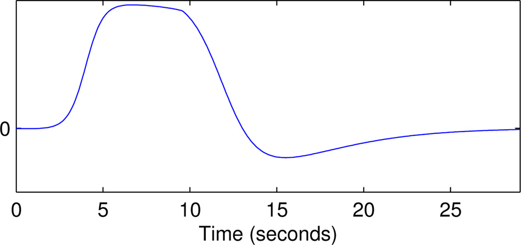
A combination of sigmoid functions was used to emulate the HRF (Fig. 2) with SNR = 1.2 equivalent to estimates from real data.

Figure 2.

HRF for simulating fMRI data, defined using a combination of sigmoid functions.

From (12), SNR is calculated as ${\sigma }_s^2/{\sigma }_v^2$. Accounting for the inconsistent spatial variation and large covariance between st and vt at each activated voxel, this is estimated as

$$\text{SNR}=\frac{{\sigma }_s^2}{{\sigma }_v^2}\approx \frac{{\sigma }_{(s+v)}^2-{\sigma }_v^2-2\text{cov}(s,v)}{{\sigma }_v^2}$$

since ${\sigma }_s^2$ is not directly accessible from the data. We use the mean SNR over all activated voxels.

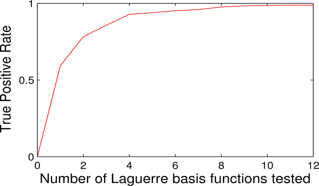
Testing for increasing numbers of extra Laguerre basis functions within the data gives an increasing true-positive rate as expected (Fig. 3). This shows that the test statistic is able to detect the presence of activation signal within real fMRI data which is significantly different to the commonly used Double Gamma model. Results are consistent under variation of simulation and analysis parameters, including using different synthetic HRF specifications than the example composite sigmoid signal of Fig. 2.

Figure 3.

Statistical power as a function of the number of basis functions tested in addition to the fitted Double Gamma Laguerre basis set.

2) Testing for Time-Varying Hemodynamic Response

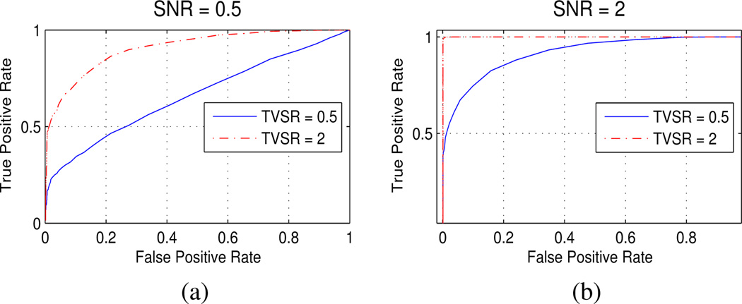
Simulation results testing for a Time-Varying Hemodynamic Response are shown as ROC curves with SNR= 0.5 (Fig. 4a) and SNR= 2 (Fig. 4b). Noise as described under the null hypothesis condition in Section IV-B includes the basic stationary activation signal. The Time-Varying Signal Ratio (TVSR) is then the variance ratio of added time-varying signal to the basic stationary activation signal. SNR is calculated as the ratio

$$\frac{{\sigma }_{\text{Time-varying activation signal}}^2+{\sigma }_{\text{Stationary-time activation signal}}^2}{{\sigma }_{\text{Other noise terms}}^2}$$ (14)

Figure 4.

ROC curves of simulation results for the algorithm testing for presence of Time-Varying (non-stationary) Hemodynamic Response in the SNR range of [0.5,2], equating to real data; see (14). These results from an event-type stimulus pattern are consistent with those from an extended block-style stimulus.

Typical SNR and TVSR values measured from real data are both between [0.5, 2], with a mean SNR of 1.2. While the test statistic calculation incorporates HRF parameters tapered by a cosine function, the Time-Varying signals embedded in simulated data have weighting corresponding to calculated values from real data, with the cumulative signal variance scaled to the desired SNR as in (14). The results in Fig. 4 indicate that the algorithm is effective, since a threshold applied at α = 0.01 of the χ² distribution with Bonferroni correction gives no false positive detection within the parameter test range equating to real data, although there is some loss of power at low SNR. Results are consistent under variation of parameters.

3) Testing for BOLD Response Non-Linearity

Data simulation involved adding increasing amounts of non-linear component to the resting state fMRI data. SNR is calculated as

$$\frac{{\sigma }_{\text{Non-linear signal component}}^2}{{\sigma }_{\text{Linear}+\text{other noise terms}}^2}$$

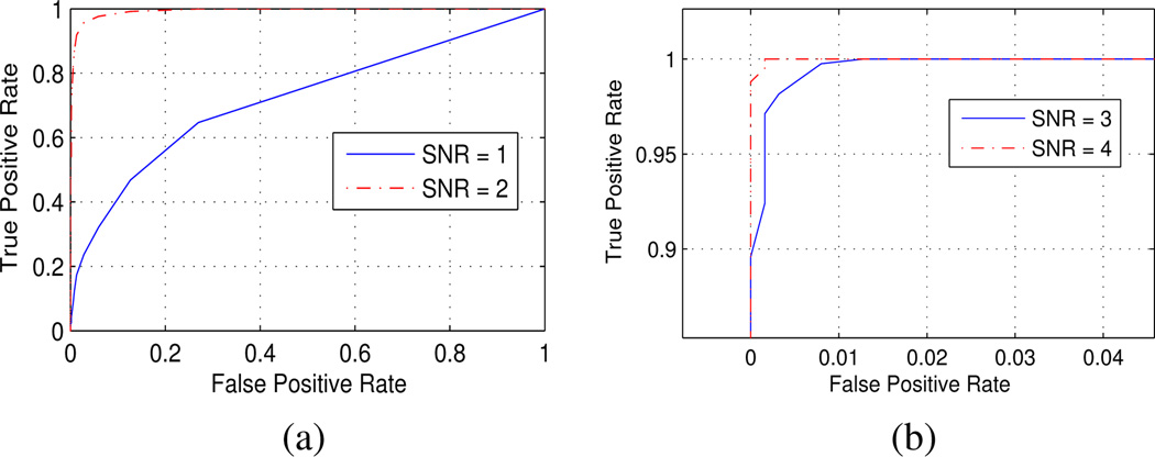
where we use the same physiologically based nonlinear model as [7] with corresponding embedded weightings for linear terms. Simulation results in Fig. 5 show the test is effective for a realistic range of SNR values, SNR = [1,4]. Results are consistent under variation of simulation and analysis parameters.

Figure 5.

ROC curves for the detection of non-linear component of fMRI signal. False positive rate is negligible for threshold α = 0.01. Simulated SNR range is comparable to real data. Plot axes are scaled in (b).

B. Single Subject Real Data

Here we describe detailed results from a single fMRI scan which is representative of the multi-subject results in Section V-C.

Data is from a combined visual/motor experiment solving simple mathematical calculation. Four-digit numbers were presented on a screen until the subject indicated a response (sum of two numbers being higher/lower than a third) by pressing one of two buttons with the right index finger, at which point the visual stimulus was removed. Data was acquired using a 3T Philips ‘Achieva’ MRI scanner with 2.000s TR; voxel size (3.125 × 3.125 × 5) millimetres, volume dimensions 61 × 50 (×28 slices); 335 temporally sampled volumes. Data was preprocessed using SPM8 (www.fil.ion.ucl.ac.uk/spm/) without spatial or temporal smoothing.

The input stimulus is modeled as an impulse at the time of button press, to model the decision-making process in the experiment. Model anomalies are also detected when input stimulus is modeled as an impulse at the time of visual presentation; however we exclude those results for clarity as they are largely similar to those included.

1) Testing for Double Gamma HRF

Here the LM-anomaly statistic is used to test whether the Double Gamma HRF is a valid impulse response model for BOLD activation.

In addition to the LM-anomaly map, we show results from conventional fMRI tests for BOLD activation. For clarity we have fitted the activation model under both the null and alternative hypotheses; but we emphasise that detecting model violation only requires fitting under the null. We have shown fitting under the alternative here purely for comparison.

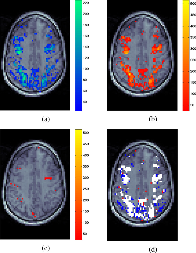
Fig. 6a shows the LM-anomaly map for the Double Gamma HRF which detects substantial areas of model violation within the data.

Figure 6.

Fig. (a) shows the LM-anomaly map testing for violation of the Double Gamma HRF. Activation maps are shown for the same data slice calculated using (b) the nonparametric Laguerre HRF basis set and (c) the Double Gamma HRF specification. Colours represent significance levels above a detection threshold of α = 0.01. Fig. (d) shows a map of voxels detected separately by the Double Gamma LM-anomaly test statistic (blue), the conventional Least-Squares activation test using nonparametric Laguerre HRF specification (red) and both (white).

The presence of anomaly in Fig. 6a is well explained by the discrepancy between activation maps generated from different model fits. The test for activation using the nonparametric Laguerre-polynomial HRF specification (i.e. the alternative hypothesis condition, H₁) shows extensive areas of detected BOLD signal (Fig. 6b); however the activation test under H₀, using the common SPM Double Gamma HRF specification detects almost no voxels (Fig. 6c).

Fig. 6d shows the anomaly corresponds almost completely to those areas detected by the conventional activation test statistic using the nonparametric Laguerre HRF specification. This indicates that the conventional method of testing for BOLD activation using the Double Gamma HRF has failed catastrophically. The SPM Double Gamma function is therefore insufficient as a model for hemodynamic BOLD signal present within this data.

2) Testing for Time-Varying Hemodynamic Response

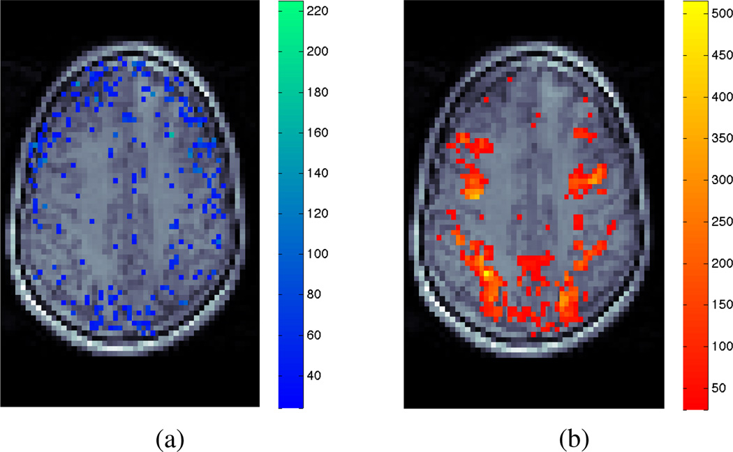
The real data results from the LM-anomaly map show model violation distributed across the brain volume (Fig. 7a). Although the areas of violation are predominantly different to those areas detected by the standard BOLD activation test (Fig. 7b), there are also areas of overlap between the activation and anomaly maps. These results indicate the BOLD activation test may include false-negative and false-positive errors within the calculated activation map.

Figure 7.

LM-anomaly map for the presence of Time-Varying HR in real data (a), in conjunction with the typical Least-Squares test statistic for BOLD activation (b) of the same data slice calculated using the nonparametric Laguerre HRF specification. Colours represent significance levels above a detection threshold of α = 0.01.

Furthermore, the pattern of detected model violation in the LM-anomaly map is similar to a motion artefact pattern, which suggests an additional explanation of the diagnostic results: that inadequate motion-correction during preprocessing has let time-varying signal characteristics remain. We estimate the extent of this effect by separately applying the LM-anomaly test with an augmented model which includes movement parameters calculated during preprocessing. The Time-Varying HRF test then detects fewer anomaly voxels when including the movement measurements in the model. Importantly, this possible preprocessing error would not have been detected without this diagnostic test, since the accompanying BOLD activation test statistic map does not suggest any such movement errors (whether or not movement regressors are included in the model).

Regardless, the results indicate a need for further examination of the data and possibly the use of a time-varying activation model in subsequent analyses.

3) Testing for BOLD Response Non-Linearity

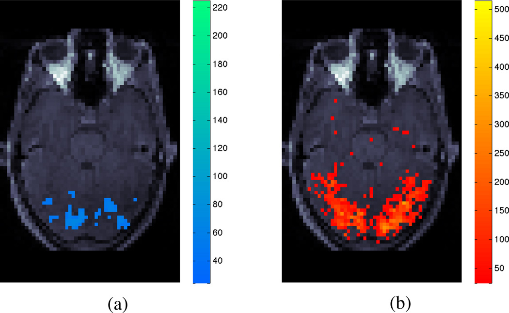
Results from the real data are shown in Fig. 8. The LM-anomaly map shows the nonlinear BOLD signal component present within cerebellum and lower visual cortex. Since this area corresponds with some, but not all, of the area detected by conventional activation statistic, there may be some false positive and/or false negative detections due to the model violation; the activation statistic is not reliable and we need to develop a procedure that allows for non-linearity in order to properly analyse the data.

Figure 8.

LM-anomaly map for the presence of Non-Linear component in fMRI signal (a), in conjunction with a linear BOLD activation test statistic of the same slice (b). Colours represent significance levels above a detection threshold of α = 0.01 for both plots.

Along with the plausible pattern of BOLD activation within visual cortex (shown in Fig. 8b), the activation statistic detects distributed voxels across the entire cerebellum. While such extended cerebellar activation is not impossible, only focal activation patterns would be expected given the design of the experiment [35]. The LM-anomaly statistic also detects focal cerebellar model violation. These results further challenge the validity of the basic activation model from a physiological viewpoint.

C. Multiple Subject Real Data

To demonstrate the general application and importance of these diagnostic tests in fMRI, we analysed data from four different experiments for a total of 370 individual fMRI data volumes; refer Table (I). The data were selected to represent a range of fMRI experiment types and input stimulus patterns (both block- and event-type) with varying complexity; three are from published work, publicly accessible at the fMRI Data Center repository (www.fmridc.org/, Item numbers: 2-2005-119FM [36]; 2-2005-119AG [37]; 2-2005-1198T [38]) and one is from an unpublished study at Neuroscience Research Australia (NeuRA) on presentation of pseudo-homophones with associated decision making regarding the validity of the words. Tests were conducted with the same input stimulus patterns as analysed in published work, and all relevant stimulus patterns for the unpublished data.

Table 1.

Meta-data for multiple subject experimental data.

Data Set	−119FM	−119AG	−1198T	NeuRA
Number of subjects	16	25	19	35
Sessions / Subject	3	4	8	2
Input stimulus conditions / Session	4	2	3	5
Temporally scanned volumes / Session	96	93	74	524
Total scanning time / Session (seconds)	384	232	222	1055

As summarised in Table (II), the cumulative results from all experiments show widespread violations in basic model assumptions for these data. The three LM-anomaly diagnostic tests were applied 1198 times each, across all applicable combinations of subject, intra-subject session and input-stimulus pattern. We reviewed each of the 3594 anomaly maps individually and excluded the 21% of results where the anomaly existed only in non-brain areas, e.g. venous sinuses. We manually reviewed the data instead of applying automatic brain extraction algorithms due to the infeasibility of adjusting the associated tuning parameters for such large amounts of data, which would otherwise constrain some fMRI volumes to contain non-brain voxels or remove some valid cortical data.

Table II.

Summary results for multiple subject data, showing the number of tests which detected some model anomaly within a particular fMRI data volume, as a fraction of the number of tests conducted for all appropriate combinations of subject/session/stimulus-condition.

Data Set	Test$(\frac{\#\mathit{\text{failed}}}{\#\mathit{\text{tested}}})$			Total volumes containing anomaly
	Double Gamma HRF	BOLD Non- linearity	Time- Varying HR
−119FM	73/192	0/192	111/192	184/576
−119AG	109/200	0/200	134/200	243/600
−1198T	434/456	28/456	448/456	910/1368
NeuRA	58/350	0/350	330/350	388/1050
			Total:	1725/3594

In total, 1725/3594 ≈ 48% of all tests detected model violation somewhere within the particular fMRI brain volume. Only 121/1198 ≈ 10% combinations of subject/session/stimulus-condition did not violate any model assumptions for any of the three LM-anomaly tests conducted.

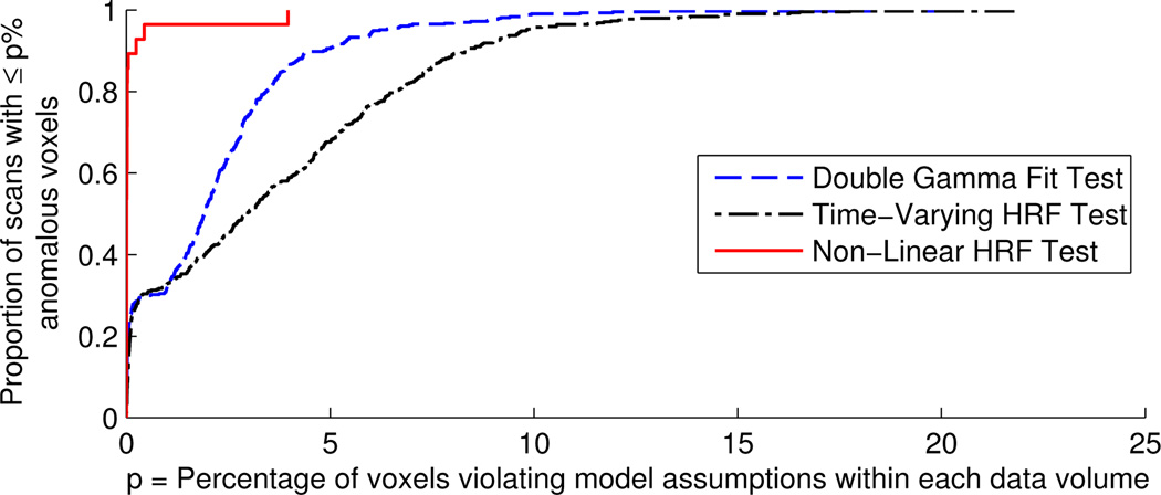
Results for the detection rate of anomaly voxels in the largest data set (Fig. 9) show that the Time-Varying HRF and Double Gamma HRF models are violated in many voxels, across extensive areas of the brain, in a large proportion of those scanning sessions. The Non-Linear HRF model is violated in only few voxels, in a small proportion of the fMRI data volumes from that experiment.

Figure 9.

Cumulative distributionn of anomaly voxel detection rate within fMRI data set −1198T.

Including movement measurements from preprocessing as extra parameters in the fMRI model (as in results Section V-B2) affects the detection of model violation only in the NeuRA data; the rate of anomaly detection reported in Table (II) across all tests for NeuRA data is 24% less than when movement parameters are excluded from the fMRI model. Reviewing the NeuRA data reveals sparse anomaly patterns around the edge of a small proportion of scans which could be representative of motion artefact, similar to the single subject test for Time-Varying HRF (Section V-B2). Anomaly maps from the 119FM, 119AG and 1198T experiments do not appear to contain motion artefact.

VI. Discussion

We have shown that applying Lagrange Multiplier diagnostic tests to fMRI data consistently identifies violations in model assumptions. This confirms the necessity of rigorous model criticism for fMRI analysis.

The FMRIDC data sets contain multiple scanning sessions for each subject performing identical experiments. Examining the patterns of model violations detected reveals strong consistency in results between repeated sessions; such that exactly replicating an experiment in separate scanning sessions usually gives the same decision on whether the basic fMRI model has been violated somewhere within the data volume. This consistency within results between sessions reaffirms the necessity of performing further analysis even in cases where only a few voxels are detected as violating model assumptions for a given LM-anomaly test.

The pattern of detected anomaly varies between experiments, subjects and stimulus conditions but is empirically consistent within each of those factors for these particular data. In particular the anomaly maps from experiments 119AG and 1198T show particularly clustered patterns of anomaly corresponding variously with those areas of brain identified in the published work as well as other areas of cortex. Anomaly maps from the 119FM and NeuRA experiments show qualitatively sparse anomaly patterns distributed throughout the particular brain volumes with less clustering of voxels. The model violation appearing to be induced from physical motion artefact in the NeuRA data is equally important and relevant as those anomalies from a physiological origin, since this source of error may not have been visually apparent in subsequent BOLD activation maps.

The discrepancy in observing apparent motion artefact between different experiments could be explained by the large differences in scanning time per session (Table I) between the NeuRA and FMRIDC data. We expect a longer cumulative scanning time to give rise to more movement artefact in fMRI data. This is observed in the data analysed herein.

Detailed results from the single data volume in Section V-B demonstrate a typical diagnostic analysis.

The experiment involved various cognitive activities from the time of stimulus (observing numbers) to making a decision (button press). Previous analyses for BOLD signal within this data [15] had shown cognitive activation in expected areas of visual cortex, motor cortex and medial frontal lobe. The results presented herein demonstrate the violation of three common fMRI model assumptions in parts of this particular data volume, indicating a need for further analysis using more appropriate models.

It is particularly interesting that a conventional test for BOLD activation using the nonparametric continuous Laguerre polynomial basis set for the HRF model detects activation in almost exactly the same areas as the LM-anomaly map for violation of the SPM Double Gamma model. In contrast, the conventional BOLD activation test using the SPM Double Gamma HRF detects almost no activation at all. Again the point here is that with almost no extra computation the anomaly map is showing that the SPM Double Gamma fails badly on this data. The Laguerre-zis happening in this case.

It is important to reiterate that the Double Gamma anomaly test is not affected by temporal drift artefact within the data, since that effect is included in the null hypothesis model. Other possible confounding factors such as Time-to-Onset delay of the HRF (see [15]) are assumed to be zero in both the Laguerre and Double Gamma models, so the model comparison is not affected. We note that this analysis does not use the exact same processing pipeline as SPM software, due to our slightly different noise modelling and test statistic threshold selection. However the analysis is consistent since we use the same noise model throughout all our analyses. Therefore the Double Gamma LM test results only indicate model violation for the exact SPM Double Gamma HRF specification and do not reflect on the efficacy of other aspects of SPM software analysis. Equivalent LM model violation tests can easily be designed for other Double Gamma HRF specifications.

An obvious interpretation of LM-test model violation results is to show possible areas of false-positive activation detection, when LM-anomaly maps overlap with activation maps. However it is equally important to consider the indications of false-negative results, arising when a region of anomaly does not overlap with detected BOLD activation regions; lack of activation detection may mean some anomaly suppresses it as in the Double Gamma case above.

Our test for BOLD signal non-linearity is based on a physiologically motivated non-linear model of behaviour within the brain, estimating BOLD signal as an interaction between blood volume and blood flow. Although this is a viable model, further research has since extended and refined understanding of non-linear BOLD behaviour (e.g. [39], [40]) as well as the non-linear adaptation of raw neural signal components [41]. It would be interesting to test and compare the appropriateness of such advanced non-linear models using Lagrange Multiplier anomaly tests, further exploring the relationship between multiple stimuli, study design, scan parameters and inter-session variability.

To the best of our knowledge there are no existing theoretical tests for the presence of BOLD signal non-linearity. Volterra characterisation of the non-linear Balloon model [39] treats the hemodynamic system as a black box, hence only judging the non-linearity fit through empirical comparison of the model and associated Volterra series expansion. In contrast, the LM method directly and quantitatively tests specific model characteristics, without needing to actually fit the alternative model.

Other future development of Lagrange Multiplier methods could include testing for fMRI model violation in such assumptions as spatial independence, validity of the ‘Double Gamma with temporal derivative’ HRF specification and stationary noise distributions.

In the examples presented, the model assumptions are not violated at every ‘active’ voxel which supposedly contains relevant BOLD signal. Nevertheless we suggest that data showing any model violation should be re-analysed using more advanced methodology appropriate to the types of model violations found. As outlined in Section III-D, the alternative model is specified already as part of the anomaly test derivation.

Fitting that alternative model (e.g. for subsequent BOLD activation testing if that is the aim of the experiment) can present challenges depending on the circumstance. Mainstream fMRI software packages offer some choice in model selection, e.g. using a FIR model for the HRF estimation; however many suitable model choices are not straightforward to implement or are available only from in-house software development. This presents an ongoing challenge to provide suitable, accessible software for the fMRI community.

VII. Conclusions

In this paper we have developed an approach to testing for model inadequacies or anomalies in fMRI analysis. The method, based on Lagrange Multiplier hypothesis tests, requires only that a standard fMRI model be fitted. Using this, minor additional computations are made to produce an ‘anomaly’ map showing where model violations occur.

Almost any kind of model anomaly can be investigated. It is required only that the alternative hypothesis be specified in terms of a statistical model, then a test statistic can be generated based on the Lagrange multiplier methodology. We have illustrated the process with three examples: a test for the validity of the Double Gamma HRF, a test for the presence of non-linearity within the HRF and a test for a time varying HRF. By analysing a large amount of data we found widespread model violations in at least two of these cases.

If model anomalies are detected using these diagnostic tests, the tested models are invalid at those voxels. Further fMRI analysis requires a different model be fitted, e.g. the model specified under the alternative hypothesis.

Finally our extensive data analysis has clearly demonstrated that model criticism needs to become a standard part of fMRI data analysis; Lagrange Multiplier methods provide a cheap and informative way of helping to accomplish that.

Appendix

Here we derive the coefficients for a continuous time Laguerre polynomial basis expansion of the HRF.

We first specify a weight function w^α(τ) = τ^αe^−τ where α is user chosen; we take it to be an integer.

The Laguerre polynomials $L_j^{(\alpha )}(\tau )$ are jth order polynomials determined by the requirement of being orthogonal with respect to the weight function w ^α(τ) i.e.

$${\int }_0^{\infty }{L}_n^{(\alpha )}(\tau )L_j^{(\alpha )}(\tau )w^{\alpha }(\tau )d\tau ={\delta }_{n,j}\frac{(n+\alpha )!}{n!}$$

We now expand the HRF as $h(\tau )={\sum }_{j=0}^{\infty }{\beta }_j^{(\alpha )}{L}_j^{(\alpha )}(\tau )w^{\alpha }(\tau )$ where ${\beta }_j^{(\alpha )}$ are coefficients to be found. If h(τ) is known these are found as follows,

$$\frac{n!}{(n+\alpha )!}{\int }_0^{\infty }h(\tau )L_n^{(\alpha )}(\tau )d\tau =\frac{n!}{(n+\alpha )!}\sum _{j=0}^{\infty }{\beta }_j^{(\alpha )}\int L_n^{(\alpha )}(\tau )L_j^{(\alpha )}(\tau )w^{\alpha }d\tau =\sum {\beta }_j^{(\alpha )}{\delta }_{n,j}={\beta }_n^{(\alpha )}$$ (15)

If h(τ) is unknown we truncate the series to q + 1 terms and estimate the coefficients by maximum likelihood.

For the SPM Double Gamma, we choose α = 5 which gives the most efficient derivation; so h(τ) = τ⁵e^−τ(a − bτ¹⁰) where $a=\frac{1}{\mathrm{\Gamma }(6)},b=\frac{1}{6\mathrm{\Gamma }(16)}$.

Then we can find the coefficients using the monomial expansion in terms of continuous Laguerre Polynomials [29],

$${\tau }^n=n!\sum _{i=0}^n{(-1)}^i\left(\begin{array}{c}n+\alpha \\ n-i\end{array}\right)L_i^{(\alpha )}(\tau )$$ (16)

and substituting it into (15). This yields ${\beta }_m^{(5)}=0,m>10$ and

$${\beta }_m^{(5)}=\left(\frac{{\delta }_{m,0}}{\left(\begin{array}{c}m+5\\ m\end{array}\right)\mathrm{\Gamma }(6)}\right)-\left(\frac{10!{(-1)}^m\left(\begin{array}{c}15\\ 10-m\end{array}\right)\mathrm{\Gamma }(m+6)}{\left(\begin{array}{c}m+5\\ m\end{array}\right)\mathrm{\Gamma }(6)\mathrm{\Gamma }(16)m!6}\right),m\le 10$$ (17)

We denote the Double Gamma coefficients calculated in (17) as ρ_m. We thus denote in general ${\beta }_m^{(5)}\text{as}{\beta }_m$.

References

- 1.Box G, Jenkins G. Time series analysis: Forecasting and control. San Francisco: Holden-day; 1970. [Google Scholar]
- 2.McCullagh P, Nelder J. Generalized linear models. London: Chapman Hall; 1989. [Google Scholar]
- 3.Ryan T. Modern regression methods. Wiley-Interscience; 2009. [Google Scholar]
- 4.Boynton G, Engel S, Glover G, Heeger D. Linear Systems Analysis of Functional Magnetic Resonance Imaging in Human V1. Journal of Neuroscience. 1996;vol. 16(no. 13):4207–4221. doi: 10.1523/JNEUROSCI.16-13-04207.1996. [DOI] [PMC free article] [PubMed] [Google Scholar]
- 5.Vazquez A, Noll D. Nonlinear Aspects of the BOLD Response in Functional MRI. Neuroimage. 1998;vol. 7(no. 2):108–118. doi: 10.1006/nimg.1997.0316. [DOI] [PubMed] [Google Scholar]
- 6.Friston K, Josephs O, Rees G, Turner R. Nonlinear event-related responses in fMRI. Magnetic Resonance in Medicine. 1998;vol. 39(no. 1):41–52. doi: 10.1002/mrm.1910390109. [DOI] [PubMed] [Google Scholar]
- 7.Solo V, Purdon P, Weisskoff R, Brown E. A signal estimation approach to functional MRI. IEEE Transactions on Medical Imaging. 2001;vol. 20(no. 1):26–35. doi: 10.1109/42.906422. [DOI] [PubMed] [Google Scholar]
- 8.Purdon P, Solo V, Weisskoff R, Brown E. Locally Regularized Spatiotemporal Modeling and Model Comparison for Functional MRI. Neuroimage. 2001;vol. 14(no. 4):912–923. doi: 10.1006/nimg.2001.0870. [DOI] [PubMed] [Google Scholar]
- 9.Aguirre G, Zarahn E, D’Esposito M. The Variability of Human, BOLD Hemodynamic Responses. Neuroimage. 1998;vol. 8(no. 4):360–369. doi: 10.1006/nimg.1998.0369. [DOI] [PubMed] [Google Scholar]
- 10.Monti M. Statistical analysis of fmri time-series: A critical review of the glm approach. Frontiers in human neuroscience. 2011;vol. 5:28. doi: 10.3389/fnhum.2011.00028. [DOI] [PMC free article] [PubMed] [Google Scholar]
- 11.Luo W, Nichols T. Diagnosis and exploration of massively univariate neuroimaging models. NeuroImage. 2003;vol. 19(no. 3):1014–1032. doi: 10.1016/s1053-8119(03)00149-6. [DOI] [PubMed] [Google Scholar]
- 12.Razavi M, Grabowski T, Vispoel W, Monahan P, Mehta S, Eaton B, Bolinger L. Model assessment and model building in fmri. Human brain mapping. 2003;vol. 20(no. 4):227–238. doi: 10.1002/hbm.10141. [DOI] [PMC free article] [PubMed] [Google Scholar]
- 13.Loh J, Lindquist M, Wager T. Residual analysis for detecting mis-modeling in fmri. Statistica Sinica. 2008;vol. 18:1421–1448. [Google Scholar]
- 14.Long CJ, Brown EN, Bullmore E, Solo V. Proc HBM03 Conference. Organisation for Human Brain Mapping; 2003. Lagrange multipliers in fmri part(i): Signal detection in unidentified models. [Google Scholar]
- 15.Solo V, Cassidy B, Long C, Rae C. Time-to-onset latency in fMRI: Fast detection of delayed activation. Acoustics, Speech and Signal Processing (ICASSP), 2011 IEEE International Conference on. 2011:725–728. [Google Scholar]
- 16.Silvey S. The Lagrangian multiplier test. The Annals of Mathematical Statistics. 1959:389–407. [Google Scholar]
- 17.Breusch T, Pagan A. The Lagrange multiplier test and its applications to model specification in econometrics. Review of Economic Studies. 1980;vol. 47(no. 1):239–253. [Google Scholar]
- 18.Engle R. Wald, likelihood ratio, and Lagrange multiplier tests in econometrics. Handbook of econometrics. 1984;vol. 2:775–826. [Google Scholar]
- 19.Box G, Draper N. Empirical model-building and response surfaces. John Wiley & Sons; 1987. [Google Scholar]
- 20.Draper N, Smith H. Applied regression analysis. 3rd ed. New York: Wiley; 1998. [Google Scholar]
- 21.Wooldridge J. Introductory econometrics: A modern approach. 4th ed. 2009. South-Western Pub. [Google Scholar]
- 22.Engle R. A general approach to Lagrange multiplier model diagnostics. Journal of Econometrics. 1982;vol. 20(no. 1):83–104. [Google Scholar]
- 23.Pawitan Y. In all likelihood: statistical modelling and inference using likelihood. Oxford University Press; 2001. [Google Scholar]
- 24.Buse A. The likelihood ratio, Wald, and Lagrange multiplier tests: An expository note. American Statistician. 1982:153–157. [Google Scholar]
- 25.Aitchison J, Silvey S. Maximum-likelihood estimation of parameters subject to restraints. The Annals of Mathematical Statistics. 1958;vol. 29(no. 3):813–828. [Google Scholar]
- 26.Brillinger D. Time Series: Data Analysis and Theory. San Francisco: Holden-Day; 1981. [Google Scholar]
- 27.Bonferroni C. Teoria statistica delle classi e calcolo delle probabilita. Seeber: Libreria internazionale; 1936. [Google Scholar]
- 28.Birn R, Bandettini P, Cox R, Shaker R. fmri during stimulus correlated motion and overt subject responses using a single trial paradigm. Proceedings of ISMRM Sixth Scientific Meeting, Sydney. 1998;vol. 159 [Google Scholar]
- 29.Olver F, Lozier D, Boisvert R, Clark C. NIST handbook of mathematical functions. 2010 [Google Scholar]
- 30.Lehovich A, Barrett H, Clarkson E, Gmitro A. Information Processing in Medical Imaging. Springer; 2001. Estimability of Spatio-temporal Activation in fMRI; pp. 259–271. [Google Scholar]
- 31.Burock M, Dale A. Estimation and detection of event-related fMRI signals with temporally correlated noise: A statistically efficient and unbiased approach. Human Brain Mapping. 2000;vol. 11(no. 4):249–260. doi: 10.1002/1097-0193(200012)11:4<249::AID-HBM20>3.0.CO;2-5. [DOI] [PMC free article] [PubMed] [Google Scholar]
- 32.Solo V, Long C, Brown E, Aminoff E, Bar M, Saha S. FMRI signal modeling using Laguerre polynomials, in. IEEE International Conference on Image Processing. 2004:2431–2434. [Google Scholar]
- 33.Schwarz G. Estimating the dimension of a model. The annals of statistics. 1978;vol. 6(no. 2):461–464. [Google Scholar]
- 34.Dunkl C, Xu Y. Orthogonal polynomials of several variables. Cambridge Univ Pr; 2001. [Google Scholar]
- 35.Stoodley C. The cerebellum and cognition: evidence from functional imaging studies. The Cerebellum. 2011:1–14. doi: 10.1007/s12311-011-0260-7. [DOI] [PubMed] [Google Scholar]
- 36.Kan I, Kable J, Van Scoyoc A, Chatterjee A, Thompson-Schill S. Fractionating the left frontal response to tools: dissociable effects of motor experience and lexical competition. Journal of cognitive neuroscience. 2006;vol. 18(no. 2):267–277. doi: 10.1162/089892906775783723. [DOI] [PubMed] [Google Scholar]
- 37.Kirchhoff B, Schapiro M, Buckner R. Orthographic distinctiveness and semantic elaboration provide separate contributions to memory. Journal of cognitive neuroscience. 2005;vol. 17(no. 12):1841–1854. doi: 10.1162/089892905775008670. [DOI] [PubMed] [Google Scholar]
- 38.Venkatraman V, Siong S, Chee M, Ansari D. Effect of language switching on arithmetic: A bilingual fmri study. Journal of Cognitive Neuroscience. 2006;vol. 18(no. 1):64–74. doi: 10.1162/089892906775250030. [DOI] [PubMed] [Google Scholar]
- 39.Friston K, Mechelli A, Turner R, Price C. Nonlinear responses in fmri: the balloon model, volterra kernels, and other hemodynamics. NeuroImage. 2000;vol. 12(no. 4):466–477. doi: 10.1006/nimg.2000.0630. [DOI] [PubMed] [Google Scholar]
- 40.Johnston L, Duff E, Mareels I, Egan G. Nonlinear estimation of the bold signal. NeuroImage. 2008;vol. 40(no. 2):504–514. doi: 10.1016/j.neuroimage.2007.11.024. [DOI] [PubMed] [Google Scholar]
- 41.Logothetis N. The underpinnings of the bold functional magnetic resonance imaging signal. The Journal of Neuroscience. 2003;vol. 23(no. 10):3963. doi: 10.1523/JNEUROSCI.23-10-03963.2003. [DOI] [PMC free article] [PubMed] [Google Scholar]