The influence of sulcus width on simulated electric fields induced by transcranial magnetic stimulation

Abstract

Volume conduction models can help in acquiring knowledge about the distribution of the electric field induced by transcranial magnetic stimulation (TMS). One aspect of a detailed model is an accurate description of the cortical surface geometry. Since its estimation is difficult, it is important to know how accurate the geometry has to be represented. Previous studies only looked at the differences caused by neglecting the complete boundary between the CSF and GM (Thielscher et al. 2011; Bijsterbosch et al. 2012), or by resizing the whole brain (Wagner et al. 2008). However, due to the high conductive properties of the CSF, it can be expected that alterations in sulcus width can already have a significant effect on the distribution of the electric field. To answer this question, the sulcus width of a highly realistic head model, based on T1-, T2- and diffusion-weighted magnetic resonance images (MRI), was altered systematically. This study shows that alterations in the sulcus width do not cause large differences in the majority of the electric field values. However, considerable overestimation of sulcus width produces an overestimation of the calculated field strength, also at locations distant from the target location.

1. Introduction

Transcranial magnetic stimulation (TMS) is a non-invasive technique that is used in a wide range of neurophysiologic and clinical studies to measure or change the excitability of specific brain areas. To do this, a very brief and strong electric current is send through a coil, which causes a time-varying magnetic field. This magnetic field consequently induces an electric field in the human head as described by Faraday’s law of induction. This current may generate neural excitation.

Although nowadays TMS is a widely used research tool, most of our knowledge is still based on experimental experience. The underlying biophysical mechanisms are not well understood yet. To adjust and improve TMS protocols, it is important to have a clear understanding of the (neural) mechanisms behind TMS. To gain insight into these mechanisms, an estimate of the induced electric field in the brain can be made with the use of computational model simulations. In the last decade several numerical models using the finite element method (FEM) (De Lucia et al. 2007; Opitz et al. 2011), the boundary element method (BEM) (Salinas et al. 2007), the independent impedance method (IIM) (De Geeter et al. 2012) or the finite difference method (FDM) (Toschi et al. 2008) have been introduced to study the spatial distribution of the induced electric field. The earliest models made use of spherical meshes (Ravazzani et al. 1996; Miranda et al. 2003) and are still used today in TMS navigation devices.

Although spherical models are still in use, more realistic head models have been developed in the last couple of years to study TMS induced electric field (Chen & Mogul 2009; Opitz et al. 2011). One of the most important aspects of a realistic head model is the inclusion of a highly accurate description of the boundary between cerebrospinal fluid (CSF) and grey matter (GM) (Bijsterbosch et al. 2012; Wagner et al. 2008; Thielscher et al. 2011). The studies with spherical models already demonstrated the importance of tissue heterogeneity (Ravazzani et al. 1996; Miranda et al. 2003), but studies using realistic head models revealed the importance of proper tissue boundary geometries (Thielscher et al. 2011).

The question addressed in this study is: how precise has the cortical surface geometry to be modelled to get an accurate estimate of the induced electric field. In previous model studies only differences caused by neglecting the complete boundary between the CSF and GM (Thielscher et al. 2011; Bijsterbosch et al. 2012), or by resizing the whole brain and including only one sulcus (Wagner et al. 2008) have been investigated. However, due to the high conductive properties of the CSF, it can be expected that even small changes in the geometry of the cortical surface will have a significant effect on the distribution of the electric field. This has already been shown to be the case in EEG source localization (Hyde et al. 2012) and to our knowledge not yet been studied for TMS.

In this study we alter the cortical sulcus width of a highly realistic tetrahedral head model in a systematic manner to verify if subtle changes in the cortical geometry have an effect on the TMS induced electric field. There are mainly two reasons for choosing the sulcus width as our primary variable and not (for example) resizing the whole cortical surface. Firstly, by only altering the sulcus width, the coil-target distance is kept constant and thereby the calculated differences are solely due to a change in cortical surface curvature. Secondly, by using this specific alteration we can study the effects of the presence of highly conductive CSF deep in the sulci, on the strength of electric fields in deeper parts of the cortex. As a by-product, the effect of the relative distribution of the CSF layer thickness, between the gyri and neighbouring sulci, can also be observed.

The insights gained by this study will help to understand the importance of correctly incorporated gyri and sulci in the cortical surface and more generally the geometrical accuracy of the cortical surface needed for TMS modelling. This information is relevant for building new individual realistic head models and setting up pipelines to construct volume conduction models for TMS simulations. The creation of a realistic head model comprises several processing steps including segmentation and possibly smoothing. Previous studies demonstrated that different software packages (FSL, SPM5 and Freesurfer) produced suboptimal GM and white matter (WM) segmentations (Klauschen et al. 2009; Shirvany et al. 2012). All three packages produce GM and WM volumes that deviate up to 10 percent from a reference template, depending on the method and image quality (Klauschen et al. 2009). Both FSL and Freesurfer reach a very high specificity for segmentation of GM and WM (almost 100 percent), but reach a much lower sensitivity (approximately 70 percent) (Shirvany et al. 2012). This means that the cortical surface can still differ several millimetres, for example in sulcus width, from reality. These segmentation errors can partially be solved with manual corrections, but this is a time consuming process. Hence, it is important to know how precise the cortical surface has to be modelled to get an accurate estimate of the induced electric field.

In addition to the scientific question at hand, this paper contains an elaborate description of the construction of a highly realistic head model that contains multiple tissues and brain anisotropy. To our knowledge, this model is one of the most accurate head models produced for TMS modelling, whereby it largely makes use of freely available software. Furthermore, a precise description of the stimulation coil is included as well. The electric field generated by the TMS coil depends on the conductive medium underneath the coil and it determines the main part of the total induced field. The importance of a realistic coil description over a simplified coil description (De Lucia et al. 2007) has already been shown in earlier studies (Salinas et al. 2007; Thielscher & Kammer 2004). The methods and head model developed for this sensitivity study can be used in future TMS investigations and can therefore be considered as valuable results in themselves.

2. Materials and Methods

2.1 Head model

A highly realistic head model was constructed using three-dimensional boundaries of eight different tissue types (skin, skull spongiosa, skull compacta, neck muscle, eye, CSF, GM and WM), which were based on T1 and T2 magnetic resonance images (MRI) scans of a healthy 25-year old male subject with 1 mm³ resolution. The construction of this standard model can be split up in five steps, namely MRI (figure 1(A)) and DTI acquisition, automatic segmentation of different tissues with manual corrections (figure 1(B)), extraction of high resolution triangular surface meshes, construction of a volume mesh with linear tetrahedral elements (figure 1(C)) and inclusion of anisotropic conductivity tensors. As explained in the Supplementary material, the WM surface was not used in the construction of the volume mesh, but afterwards to assign the resulting tetrahedrons within the brain compartment to either GM or WM. Also the cerebellum was not included in the head model. A detailed description of the standard model is added in the Supplementary Material.

Figure 1.

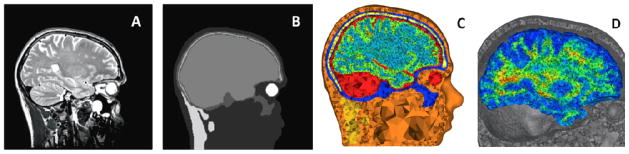
(A) A sagittal cut plane of the T2w MRI showing the different skull layers. (B) The same sagittal cut plane of the manually corrected segmentation including skin, skull compacta, skull spongiosa, neck muscle, eyes and one compartment for inner skull (CSF, GM and WM, before segmentation with Freesurfer). (C) Sagittal cut plane of the final tetrahedral volume mesh created with TetGen. The different tissue types are represented with different colours. The corresponding bulk conductivities are given in Table 1. (D) Sagittal cut plane of the brain mesh with the fractional anisotropy on a scale from 0 (blue) to 1 (red). The maximal fractional anisotropy value in the brain is 0.99 and the minimum is 0.

An important aspect of a realistic head model in TMS simulations is brain anisotropy (De Lucia et al. 2007; Opitz et al. 2011; Miranda et al. 2003). For adult human subjects, the effect of brain anisotropy on the induced electric field is mainly significant for the white matter (WM), but some smaller effects can be found for the GM as well (Opitz et al. 2011). Therefore, brain anisotropy was also included in the standard and altered models used in this study (figure 1(D)). The brain anisotropy was based on the diffusion tensors from DTI data, using the volume-normalized approach as described in (Opitz et al. 2011). The bulk conductivity values for all tissues can be found in table 1.

Table 1.

The bulk conductivity values (S/m) for all the tissue types used in the standard model.

Tissue type	Bulk conductivity (S/m)
Skin	0.465 (Wagner et al. 2004)
Skull compacta	0.007 (Akhtari et al. 2002)
Skull spongiosa	0.025 (Akhtari et al. 2002)
CSF	1.65 (Wagner et al. 2004)
Neck muscle	0.4 (Faes et al. 1999)
Eyes	1.5 (Nadeem et al. 2003)
GM	0.276 (Wagner et al. 2004)
WM	0.126 (Wagner et al. 2004)

2.2 Cortical geometry alteration

To study the effects of changes in the cortical surface geometry on the electric field, the GM surface mesh used in the standard model was altered by a process of either erosion or expansion of the gyri. The triangular surface meshes of other tissues were kept the same. For the construction of the altered surfaces, the nodes of the standard GM surface were shifted along their normal vectors relative to the surface (inward for erosion and outward for expansion). They were shifted 0.5, 1.0 and 1.5 mm in positive or negative direction. Because this alteration was applied to the whole surface and therefore also to both walls of one sulcus, the total change would be comparable to an incorrect segmentation of 3 sulci voxels in an MRI scan with 1 mm resolution. The spatial effect of 1.5 mm erosion or expansion on a specific sulcus is illustrated in Figure 2. Intersections caused by shifting the nodes were solved using open source software MeshFix (Attene et al. 2010). The expanded surface meshes had less nodes and triangles because of disappearing sulci. To avoid differences in the electric field caused by a change in CSF thickness between the top of the gyri and the skull (Bijsterbosch et al. 2012; Wagner et al. 2008) and the distance of the cortical surface to the TMS coil, the altered surfaces were up- or down-scaled to fit the dimensions of the standard GM surface again. The cortical TMS target location was set at the same location as in the standard model. This way only the differences in width of the sulci distinguish the altered models from the standard model. The altered surfaces were incorporated in new tetrahedral models and the final volume meshes had between 3.50M and 4.04M elements. The anisotropic brain conductivity tensors were mapped from the hexahedral MRI mesh onto the altered models in the same way as for the standard model (Supplementary Material). The additional elements in the expanded models were assigned the conductivity tensors from the nearest elements in the hexahedral MRI mesh.

Figure 2.

The effect of erosion and expansion on a sulcus. In brown a sulcus of the standard model is shown, in green the sulcus of a 1.5 mm eroded surface and in blue the sulcus of a 1.5 mm expanded surface. All other alterations lie between these two boundaries.

2.3 Finite element method

The finite element method is widely used to compute the spatial distribution of the electric field and current distributions that arise from electromagnetic phenomena in three-dimensional models. For the application of TMS we used the simplification of the full Maxwell’s equations by a quasi-static system wherein we neglect the displacement currents. Neglecting the displacement currents was justified in an earlier study (Wagner et al. 2004).

Consequently the total electric field E⃗ induced by the TMS coil is described by:

$$\overrightarrow{E}=-\frac{d\overrightarrow{A}}{dt}-\overrightarrow{\nabla }\mathrm{\Phi }$$ (1)

with $\frac{d\overrightarrow{A}}{dt}$ being the time-derivative of the magnetic vector field and Φ the electrical scalar potential. The first term, also called the primary component, is completely determined by the TMS coil and can be calculated at the centre of each element in the tetrahedral volume mesh. The second term, called the secondary component, describes the charge accumulation at conductivity discontinuities in the volume mesh and needs to be computed with the FEM. The primary component is computed by:

$$\frac{d\overrightarrow{A}}{dt}=\frac{{\mu }_0\text{N}\text{dI}/\text{dt}}{4\pi }\int \frac{\overrightarrow{dl}}{|\overrightarrow{r}-{\overrightarrow{r}}_0|}$$ (2)

with μ₀ the permeability of free space, N the number of windings in the TMS coil, $\frac{dI}{dt}$ the time dependent coil current, $\overrightarrow{dl}$ an infinitesimal vector representing an element of the wire through which the current passes and |r⃗ − r⃗₀| the distance between a point in space and that coil element. The spatial distribution of the primary electric field component thus fully depends on the geometry of the coil. Therefore, an accurate description of the coil should be used (Salinas et al. 2007).

Because the figure-of-eight coil can be considered the standard coil in fundamental TMS research, such a coil was simulated. The position and orientation of the coil with respect to the head were based on experimental data measured using the Localite neuronavigational system (http://www.localite.de). This coil position showed the highest motor evoked potential (MEP) in the first dorsal interosseous (FDI) muscle of the healthy 25-year old male subject and is therefore called the ‘FDI hotspot’ position.

The resulting relative spatial distribution of the field is independent of the absolute coil current. For simulations, the field distribution was scaled such that the maximum primary field strength was 300 V/m. This is approximately 45% of the maximum intensity of a biphasic pulse measured for the simulated figure-of-eight coil (Salinas et al. 2007). This intensity evoked the MEP mentioned earlier with a mean amplitude of 1.0 mV in the subject on whom the standard model is based.

The secondary component of the induced electric field is caused by the discontinuities in the conductivity σ. The induced electric field causes a current density J⃗ following Ohm’s law:

$$\overrightarrow{J}=\overrightarrow{E}\sigma$$ (3)

Perpendicular to the boundary between elements, this induced current is continuous, which yields the following constraint across boundaries:

$${\overrightarrow{J}}_1·\overrightarrow{n}={\overrightarrow{J}}_2·\overrightarrow{n}$$ (4)

When the medium is inhomogeneous, a discontinuity in the electric field occurs at the boundary between tissues with different conductivities (Miranda et al. 2003). Because the magnetic vector field is determined only by the properties of the TMS coil, this change is caused by a difference in potential gradient at the tissue boundaries.

To acquire the potential gradient in equation (1) we make use of the fact that in the quasi-static limit the divergence of the induced current has to be zero:

$$\overrightarrow{\nabla }·\overrightarrow{J}=0$$ (5)

By combining equations (1), (3) and (5) the continuity equation under quasi-static condition follows:

$$\overrightarrow{\nabla }·\left(-\sigma \frac{d\overrightarrow{A}}{dt}-\sigma \overrightarrow{\nabla }\mathrm{\Phi }\right)=0$$ (6)

The Neumann boundary condition states that no current leaves the volume conductor, so at the outer boundary we have:

$$\overrightarrow{J}·\overrightarrow{n}=0$$ (7)

This equation combined with equations (1) and (3) yields:

$$\left(\sigma \frac{d\overrightarrow{A}}{dt}\right)·\overrightarrow{n}=-\left(\sigma \overrightarrow{\nabla }\mathrm{\Phi }\right)·\overrightarrow{n}$$ (8)

The potential Φ, solved by the FEM, is then used in combination with the primary field $\frac{d\overrightarrow{A}}{dt}$ to calculate the total electric field for each element inside the volume conductor using equation (1).

The construction of the coil geometry and the placement over the models was performed with custom written MATLAB code. The calculation of the magnetic vector field was done with a custom written C++ program for each model individually following a discretized version of equation (2). The total number of wire elements (184k) was determined by doubling the number of elements step by step until the resulting magnetic vector field, calculated on the standard model, differed less than 1 percent compared to the magnetic vector field of the previous step. For the FEM calculations the freely available SCIRun 4.5 (Scientific Computing and Imaging Institute, Salt Lake City, UT) software was used. The system of linear equations was solved with a preconditioned Jacobi conjugate gradient method with residuals < 10⁻¹⁵. It took approximately 2.5 minutes to solve the system of linear equations with SCIRun on a Mac Pro, 2.66 GHz Quad-Core Intel Xeon with 16 GB memory.

The cortical erosion process can produce a very small number of elements which are less shape-regular. For example, in TetGen¹, the ratio of Q=R/L is used for determining shape-regularity with R the radius of the outer circumsphere and L the length of the shortest edge of an element. Numerical convergence properties (Braess 2007, Theorem 7.3) depend on the shape regularity of the elements. Less shape-regular elements (larger Q) lead to larger convergence constants that might result in less numerically accurate potential values within or close to the deformed elements. Furthermore, the secondary component (equation 1) is calculated by taking the gradient of the potential. The diminished accuracy of the potential values at the nodes of large-Q elements then propagates into a diminished accuracy of the potential gradient vectors. For these reasons the maximum field strength is not used as a comparison measure, but the more robust median of the 1 percent highest electric field values.

2.4 Comparison methods

The induced electric fields predicted for the altered head models were compared with the results from the standard model in two ways, namely in a cross section of the volume meshes through a sulcus near the hotspot and over the whole cortical surface. For generalization of the results found for optimal stimulation of the FDI hotspot on the left hemispheric motor cortex, the whole procedure was repeated for three more coil orientations (90, 180 and 270 degree turn compared to optimal) and three other brain areas (right hemispheric motor cortex, left hemispheric inferior frontal gyrus and left hemispheric visual cortex).

For the whole cortical surface comparisons, the electric field on the GM side of the CSF-GM boundary was used. In this way the effects of alterations in the cortical geometry on the induced field just beneath the cortical surface are compared. This is important because there is sufficient evidence that the TMS induced activation occurs mostly at the interneurons in the GM (Di Lazzaro et al. 2004). The surfaces after expansion had less nodes and triangles because of the disappearing sulci. For this reason, only the nodes in the altered model for which the original node could be located in the standard model were used in the surface comparison.

For the quantification of the difference between two models the relative difference measure (Meijs et al. 1989) and the MAG factor (Meijs et al. 1989) were used:

$$\mathit{RDM}=\sqrt{\frac{{\sum }_{i=1}^M{|{\overrightarrow{E}}_{a_i}-{\overrightarrow{E}}_{st{d}_i}|}^2}{{\sum }_{i=1}^M{\left|{\overrightarrow{E}}_{st{d}_i}\right|}^2}}$$ (9)

and

$$\mathit{MAG}=\sqrt{\frac{{\sum }_{i=1}^M{\left|{\overrightarrow{E}}_{a_i}\right|}^2}{{\sum }_{i=1}^M{\left|{\overrightarrow{E}}_{st{d}_i}\right|}^2}}$$ (10)

Here E⃗_a is the electric field on a node i in the altered model and E⃗_std the electric field on the same node i in the standard model.

3. Results

The electric field throughout the whole volume mesh was computed. Table 2 shows the median of the top 1 percent absolute field strength values in the different tissue types of all models. All models show the highest and almost identical values for the electric field in the skin and the skull compacta. The relatively small distance to the coil causes these high values within the skin. The even higher values inside the skull compacta are caused by its relatively low conductivity compared to the neighbouring tissue types (skin, skull spongiosa and CSF). Here the secondary field has its main effect. The alterations to the cortical surface do not affect the maximum field strength in the skin, skull spongiosa, neck muscle and eyes. For the skull compacta the maximum field strength increases slightly with cortical expansion.

Table 2.

The median of the top 1 percent highest electric field values (V/m), for each tissue type in the standard model and all altered models.

Median value top 1 percent highest electric field values per tissue type (V/m)
Tissue type	1.5 mm expansion	1.0 mm expansion	0.5 mm expansion	Standard model	0.5 mm erosion	1.0 mm erosion	1.5 mm erosion
Skin	159	159	159	159	159	159	159
Skull compacta	185	183	182	182	182	182	182
Skull spongiosa	142	142	142	142	142	142	142
CSF	119	117	115	117	116	113	116
Neck muscle	7	7	7	7	7	7	7
Eyes	7	7	7	7	7	6	7
GM and WM	94	92	92	97	100	105	113

Although it is relevant to know the intensities induced in other tissue types, our main interest of course concerns the field in the brain. The alterations have an opposite effect on the electric field in the brain compared to that in the skull compacta. The maximum field strength increases with cortical erosion. A slight decrease can be seen for the brain tissue with expansion. No clear effect can be seen in the CSF.

Figure 3(A) shows a cross-section around a sulcus in the standard model. The black lines show the boundaries between the CSF and the skull and the CSF and GM. The electric field in the CSF of the sulcus is relatively low (blue colour) compared to the electric field in the brain structures (orange). The locations where the CSF is thinnest, between the cortex and the skull, have the highest field strengths. This is in accordance with previous reports (Bijsterbosch et al. 2012).

Figure 3.

(A) The electric field distributions (V/m) in a cross section of the standard model with brain anisotropy. The black lines show the boundaries between the CSF and the skull and the CSF and GM. (B) The same cross-section for an inhomogeneous brain with the bulk conductivity for GM and WM and (C) for a homogeneous brain with the GM bulk conductivity. Subsequently the cross-section for the anisotropic brain with (D) 0.5 mm erosion, (E) 1.0 mm erosion, (F) 1.5 mm erosion, (G) 0.5 mm expansion, (H) 1.0 mm expansion and (I) 1.5 mm expansion. In all panels the field strength is displayed on a scale from 0 to 150 V/m.

Figure 3(B) shows the electric field in the standard model with an inhomogeneous isotropic brain to illustrate the effect of the inclusion of brain anisotropy on the electric field. The differences (compared to figure 3(A)) are small and can mostly be found in the WM, confirming previous reports (De Lucia et al. 2007; Opitz et al. 2011). The electric field in the standard model with a homogeneous isotropic brain is shown in figure 3(C), to illustrate the effect of tissue inhomogeneity. In a homogeneous model the electric field in the deeper brain regions consists almost exclusively of the primary field, because there are no conductivity boundaries. Tissue inhomogeneity (present in figures 3(A) and 3(B)) introduces additional boundaries inside the brain because of the change in bulk conductivity for the WM region. The tissue inhomogeneity causes an increase in field strength in the gyri and in the WM beneath the gyri. The field strength decreases in the brain region beneath the sulci.

In figure 3(D–F), the effects of erosion of the cortical surface (of the standard model in figure 3(A)) are shown. When the cortical surface is eroded, more CSF is introduced and the tops of the gyri become narrower. An increase in sulcus width causes the electric field to become more focal on top of the gyri and to increase in absolute field strength at these locations. The overall effects of the alterations are mainly present in the areas close to the cortical surface. The part of the volume mesh that is distant to the CSF shows only minor or no differences compared to the standard model.

In figure 3(G–I) the effects of expansion are shown. As expected the decrease in sulcus width by expansion causes an increase in the electric field between the original gyri.

Cortical surface

The experimentally identified ‘FDI hotspot’ was located at the top of a gyrus of the hand area of the motor cortex (figure 4(A), black dot). At this location the electric field is maximal (figure 4(A)). In addition to the motor cortex, also parts of the pre-motor and sensory cortex appear to be stimulated with a similar intensity. In most cases the highest values for the electric field are located at the crowns and lips of the gyri, which is in accordance with earlier reports (Bijsterbosch et al. 2012; Thielscher et al. 2011). The median of the top 1 percent electric field values just below the cortical surface are given in table 3.

Figure 4.

Top row: (A) The induced electric field (V/m) just below the cortical surface of the standard model and (B) the areas stimulated with more than 123 V/m for the 1.5 mm expanded model (blue), the standard model (red) and the 1.5 mm eroded model (green).

Middle row: For the 1.5 mm eroded model, (C) the induced electric field (V/m), (D) the magnitude of the differences with the standard model and (E) the direction of the differences (red, the altered model has a higher electric field strength, blue the altered model has a lower electric field strength).

Bottom row: For the 1.5 mm expanded model, (F) the induced electric field (V/m), (G) the magnitude of the differences with the standard model and (H) the direction of the differences.

The differences in panels D, E, G and H are projected on the standard model surface. In panels (A, C, D, F & G) the field strength is displayed on a scale from 0 to 150 V/m.

Table 3.

The median of the top 1 percent of (1) the highest electric field values (V/m) and (2) the highest differences in the electric field values (V/m). All values are based on the cortical surface of the standard model and all altered models.

Model	Median value of the 1 percent highest electric field values (V/m)	Median value of the 1 percent highest differences in electric field values (V/m)
1.5 mm erosion	131	25
1.0 mm erosion	123	16
0.5 mm erosion	119	8
Standard	117	0
0.5 mm expansion	112	9
1.0 mm expansion	113	13
1.5 mm expansion	116	14

An increase of the sulcus width increases the area for which the induced field strength is above a certain threshold (figure 4(B)). This means that the electric field is less focal in a human brain with wide sulci compared to a brain with narrower or no gyri. Figure 4(B) shows the area with an induced field above 123 V/m. Expansion of the cortical surface has an opposite effect to erosion, but the effect is smaller.

In the eroded brain surface (figure 4(C)) the maximum field strength is increased and other peaks in the field occur at gyral lips. The wider sulci cause an increase in electric field strength at the gyral crowns and lips and a larger dispersion of high intensity field peaks. These other peaks especially occur at the new sharp gyral lips that lie distal from the FDI hotspot. Figure 4(D) shows the difference in the electric field strength at the cortical surface level between the eroded and standard model. The difference between the models is especially found at the gyral lips over a widespread area. The majority of the electrical field values differ less than 13 V/m, which is 10 percent of the maximum value in the standard model. Figure 4(E) provides information about the direction of the change in the electric field. The electric field in the eroded model is higher at the top of the gyri (red) and lower in the sulci (blue).

As was expected, expansion of the cortical surface has an opposite effect to erosion (figure 4(F-H)). The expanded brain surface shows a wide dispersion of the electric field and overall lower values on top of the gyri and higher in the (former) sulci. The median of the top 1 percent electric field values differs only moderately from the standard model (table 3), but there are clear differences in field strength locally.

Alteration magnitude

The degree of alteration in the cortical surface has an effect on the differences in the electric field compared to the standard model. A higher degree of erosion induces larger changes in the electric field compared to the field in the reference model (figure 5(A–B)). When only a small alteration of 0.5 mm is applied to the cortex, the change in field strength is less than 15 V/m for almost all locations. However, an increase in erosion to 1.0 mm or 1.5 mm introduces a large number of surface nodes whose fields differ far more than 15 V/m from the standard model. Most of these larger differences apply to the nodes within a range of 30 mm to the cortical hotspot (figure 5(B)).

Figure 5.

Two logarithmic histogram plots that show the differences in electric field strength for the nodes of the cortical surface with eroded sulci compared to the standard cortical surface. Only differences up to 35 V/m (the far majority) are shown. (A) The differences between all comparable nodes in the standard model and the nodes in a model with 0.5 mm erosion (green), 1.0 mm erosion (red) and 1.5 mm erosion (blue). (B) The same comparison, but only for the nodes that are within a 30 mm radius of the cortical FDI hotspot.

The RDM is a measure for the difference over all surfaces nodes. The value for the cortical surface demonstrates the dependency on the degree of alteration. Table 4 shows that for the eroded model the RDM value of the cortical surface can go up to 0.22 for an alteration of 1.5 mm. The RDM value has a clear correlation with the magnitude of the alteration: the bigger the erosion, the bigger the value. The comparison between the standard model and the expanded models shows a less strong dependency. The reason is that the nodes in the sulci are removed after expansion and only the nodes at the top of the gyri can be compared. This causes a ceiling effect in the differences between the expanded and standard model. The MAG values show that the field strength increases with erosion, while the strength decreases with expansion.

Table 4.

The RDM (equation 9) and MAG (equation 10) values calculated over the cortical surface between the altered models and the standard model. The calculations are repeated for stimulation over 4 different brain areas (left hemispheric M1, right hemispheric M1, left hemispheric inferior frontal gyrus (IFG) and left hemispheric visual cortex (OC)). For the left hemispheric M1, 2 coil orientations are presented.

RDM and MAG value
Alteration	Left M1				Right M1		Left IFG		Left OC
	Optimal orientation		+90 deg		Optimal orientation		Optimal orientation		Optimal orientation
	RDM	MAG	RDM	MAG	RDM	MAG	RDM	MAG	RDM	MAG
1.5 mm erosion	0.22	1.11	0.20	1.09	0.21	1.10	0.20	1.09	0.19	1.09
1.0 mm erosion	0.14	1.06	0.13	1.05	0.13	1.06	0.13	1.05	0.12	1.05
0.5 mm erosion	0.08	1.03	0.07	1.02	0.07	1.03	0.07	1.02	0.07	1.02
0.5 mm expansion	0.08	0.99	0.08	0.99	0.07	0.98	0.07	0.99	0.07	0.98
1.0 mm expansion	0.11	0.97	0.10	0.97	0.10	0.97	0.10	0.97	0.10	0.97
1.5 mm expansion	0.10	0.96	0.10	0.96	0.09	0.96	0.09	0.97	0.09	0.96

Similar RDM and MAG values are found for three more TMS coil orientations and for three different brain areas. Only two coil orientations are shown in Table 4, because turning the TMS coil 180 degrees and from −90 to +90 degrees produced the same RDM and MAG values, as would be expected.

4. Discussion

The results from this study show that most of the changes in the simulated electric field caused by a slight alteration to the cortical surface are small and rather patchy. Alterations in sulcus width up to 1.5 mm do not drastically change the electric field distribution globally, as has been shown before (Laakso & Hirata 2012). These results would indicate that for a global approximation of the electric field the incorporation of an accurate description of the sulci (+/− 3 mm in width) is not highly important. However, incorporation of wide sulci (and consequently thin gyri) will cause high electric field values at gyri more distant from the stimulation target. This means that for estimations about the maxima in the electric field, these alterations may be relevant.

The effects of alteration on the electric field

In all model versions, the electric field is highest at the top and lips of the gyri, which is in accordance with the results of previous studies (Thielscher et al. 2011; Bijsterbosch et al. 2012). As the distance between the skull-CSF and CSF-GM boundary decreases, the electric field strength at these boundaries increases. This effect causes the highest peaks in electric field to occur at the gyral crowns and lips (figure 3). Locations with lower electric field values can be found in the sulci. The largest differences caused by the cortical alterations can be found at the gyral lips. An effect was found both on field strength and on field distribution. Overall, the cortical alterations do not affect deeper brain areas. The alterations to the cortical geometry change the thickness of the gyral tops and thereby alter the length of the narrow passages between the cortex and the skull. In the case of erosion the gyral crowns decrease in width and thereby the maximum electric field strength increases at the gyral lips and at the top of the gyri as well. The opposite effect can be seen in the case of expansion. These results suggest that especially the ratio between the volume of CSF on top of a gyrus and in the neighbouring sulci has an effect on the electric field strength.

The simulations with the eroded surfaces show that a cortical surface with narrow gyri can have multiple peaks in the electric field. These can be distant from the targeted FDI hotspot (figure 4(B–C)). Most of the peaks can again be found on the crown or lips of gyri.

Neuron models

The precisely studied differences in field strength caused by the alterations may not be relevant for a global estimation of the induced electric field, but are relevant for the future combination with neuron models. For a complete understanding of TMS effects at a neuronal level, volume conduction models must be combined with neuron models (Salvador et al. 2011). But for neuron models to be of value, realistic field estimations are a condicio sine qua non.

There is evidence that the first neuronal activation by TMS, presented as I-waves in subdural recordings, takes place at the level of the interneurons in the GM (Di Lazzaro et al. 2004). Only with high stimulation intensities the direct activation of the neuronal axons is achieved, presented as D-waves, generated in or close to the WM. The effects of cortical alteration are mainly found near the CSF-GM boundary and will therefore probably only affect the electric field that produces the I-waves. There is also evidence that the actual activation of neurons is directly related to the electric field (i.e. the gradient in the potential) along the axon (Roth & Basser 1990). This means that cortical sites that have high electric field strength parallel to an axon are the most likely locations to become activated. Previous model studies already concluded that the sites of neuronal activation are gyral crowns with neurons that are aligned with the primary field and axon collaterals and terminations in the lip of the gyrus (Salvador et al. 2011; Silva et al. 2008). These are also the locations with the highest electric field strength in our simulations. The effect of cortical alterations on the neurons in the gyral crowns is minimal (figure 4(d) and figure 4(f)). For the axon collaterals and terminations in the gyral lips the effects are largest.

Limitations of the presented study and future model studies

A previous study showed that the resolution needed for TMS simulations is 2 mm (Laakso & Hirata 2012). In that particular study, the effects of different hexahedral grid resolutions on the calculated average TMS field strength within a specified analysis volume were reported. The authors observed no changes in the electric field due to increase in grid resolution from 0.25 mm to 2.00 mm. Our study is partially in agreement with these previous results, because globally no large differences are observed. However, our results provide additional information about local changes in the electric field that are possibly relevant for future studies with neuron models.

This study primarily looked at the influence of the effect of sulcus width in the cortical surface. To isolate the effects of erosion and expansion, we corrected the model versions for the large effect of a change in CSF thickness (Bijsterbosch et al. 2012; Wagner et al. 2008). This way also the distance of the cortical surface to the TMS coil was the same for all models.

The comparison between an isotropic and anisotropic brain was already made in earlier studies which showed that the differences caused by anisotropy were mainly present in the WM (Opitz et al. 2011). The average difference was around 8 percent in the WM and could rise up to 40 or 50 percent locally. In the GM the authors only found less than 1 percent difference between an isotropic and anisotropic brain. The sulcus width as considered in this study has its main effect on the electric field near the CSF-GM boundary, so no strong effects of brain anisotropy was to be expected. To verify that brain anisotropy has no effect on the main conclusions of this study, all comparisons have been repeated with an isotropic brain (grey and white matter). The RDM values for these comparisons are similar to the ones produced with an anisotropic brain (0.22 for 1.5 mm erosion and 0.10 for 1.5 mm expansion, Table 4) for the optimal orientation.

Permittivity has also an influence on the effective conductivity of several tissues (De Geeter et al. 2012). This would imply a scaling of some conductivities in our quasi-static model. We verified that this would not influence the main message of this study.

The WM surface was not included in the construction of tetrahedral models, because it caused too many intersections in the triangular surface meshes after the cortical alterations. Instead the WM surface was used to assign WM labels to elements in the final tetrahedral volume meshes and give them the corresponding bulk conductivity. In other studies that used a realistic head model, this WM surface was included in the construction (Opitz et al. 2011). The segmentation and construction of the WM surface with the standard software packages is subject to the same errors and difficulties as the GM surface (Klauschen et al. 2009; Shirvany et al. 2012). Therefore, the assumption can be made that alteration of this surface can also have an influence on the induced electric field. However, in this study we decided to focus only on the alterations in the GM surface, because it has the most prominent conductivity jump and is closer to the TMS coil.

A different option for a volume conductor model is a hexahedral model directly derived from the measured MRI data (De Lucia et al. 2007; Laakso & Hirata 2012). This approach allows for an easy and automated FEM mesh generation without the manual work steps involved in the construction of tetrahedral head models. However, the tissue boundaries in this kind of volume mesh will contain geometrical imperfections. This study showed that even small differences to the cortical geometry could locally induce relevant differences in the electric field distribution. A possible way to overcome imperfections of a hexahedral model could be the use of partial volume CSF modelling (Hyde et al. 2012) or geometry-adapted hexahedral meshes (Wolters et al. 2007).

Finally, the results from this study could have consequences for future patient specific models. Several brain diseases, like Alzheimer’s disease and stroke are caused by real geometrical changes in the cortex. The induced field caused by TMS in these diseased brains will therefore have a specific effect. This was found in a first simplified brain model for stroke (Wagner et al. 2006), but the present study shows that even small alterations can induce relevant effects.

5. Conclusion

In a highly realistic head model, alterations in sulcus width (up to 3 mm) do not cause large differences in the calculated electric field values for most areas of the brain. For a global approximation of the electric field, the incorporation of an accurate description of the sulci is not highly important. However, considerable overestimation of sulcus width produces an overestimation of the local field strength, also at locations distant from the cortical hotspot. This means that for estimations about the maxima in the electric field and (future) combinations with neuron models, an accurate description of the sulcus width is advisable.

References

- Akhtari M, et al. Conductivities of three-layer live human skull. Brain topography. 2002;14(3):151–67. doi: 10.1023/a:1014590923185. [DOI] [PubMed] [Google Scholar]
- Attene M. A lightweight approach to repairing digitized polygon meshes. The Visual Computer. 2010;26(11):1393–1406. [Google Scholar]
- Bijsterbosch JD, Barker AT, Lee K-H, Woodruff PWR. Where does transcranial magnetic stimulation (TMS) stimulate? Modelling of induced field maps for some common cortical and cerebellar targets. Medical & biological engineering & computing. 2012;50(7):671–681. doi: 10.1007/s11517-012-0922-8. [DOI] [PubMed] [Google Scholar]
- Braess D. Finite Elements: Theory, Fast Solvers and Applications in Solid Mechanics. Cambridge University Press; 2007. [Google Scholar]
- Chen M, Mogul DJ. A structurally detailed finite element human head model for simulation of transcranial magnetic stimulation. Journal of neuroscience methods. 2009;179(1):111–20. doi: 10.1016/j.jneumeth.2009.01.010. [DOI] [PubMed] [Google Scholar]
- De Geeter N, Crevecoeur G, Dupre L, Van Hecke W, Leemans A. A DTI-based model for TMS using the independent impedance method with frequency-dependent tissue parameters. Physics in medicine and biology. 2012;57(8):2169–88. doi: 10.1088/0031-9155/57/8/2169. [DOI] [PubMed] [Google Scholar]
- De Lucia M, Parker GJM, Embleton K, Newton JM, Walsh V. Diffusion tensor MRI-based estimation of the influence of brain tissue anisotropy on the effects of transcranial magnetic stimulation. NeuroImage. 2007;36(4):1159–70. doi: 10.1016/j.neuroimage.2007.03.062. [DOI] [PubMed] [Google Scholar]
- Di Lazzaro V, Oliviero A, Pilato F, Saturno E, Dileone M, Mazzone P, Insola A, Tonali PA, Rothwell JC. The physiological basis of transcranial motor cortex stimulation in conscious humans. Clinical Neurophysiology. 2004;115(2):255–266. doi: 10.1016/j.clinph.2003.10.009. [DOI] [PubMed] [Google Scholar]
- Faes TJC, Van der Meij HA, De Munck JC, Heethaar RM. The electric resistivity of human tissues (100 Hz–10 MHz) a meta-analysis of review studies. Physiological Measurements. 1999;1(20) doi: 10.1088/0967-3334/20/4/201. [DOI] [PubMed] [Google Scholar]
- Hyde DE, Duffy FH, Warfield SK. Anisotropic partial volume CSF modeling for EEG source localization. NeuroImage. 2012;62:2161–2170. doi: 10.1016/j.neuroimage.2012.05.055. [DOI] [PMC free article] [PubMed] [Google Scholar]
- Klauschen F, Goldman A, Barra V, Meyer-Lindenberg A, Lundervold A. Evaluation of automated brain MR image segmentation volumetry methods. Human Brain Mapping. 2009;30:1310–27. doi: 10.1002/hbm.20599. [DOI] [PMC free article] [PubMed] [Google Scholar]
- Laakso I, Hirata A. Fast multigrid-based computation of the induced electric field for transcranial magnetic stimulation. Physics in medicine and biology. 2012;57:7753–65. doi: 10.1088/0031-9155/57/23/7753. [DOI] [PubMed] [Google Scholar]
- Meijs JWH, Weier OW, Peters MJ, Van Oosterom A. Method. IEEE transactions on biomedical engineering. 1989 Oct;36:1038–1049. doi: 10.1109/10.40805. [DOI] [PubMed] [Google Scholar]
- Miranda PC, Hallett M, Basser PJ. The electric field induced in the brain by magnetic stimulation: a 3-D finite-element analysis of the effect of tissue heterogeneity and anisotropy. IEEE transactions on bio-medical engineering. 2003;50(9):1074–85. doi: 10.1109/TBME.2003.816079. [DOI] [PubMed] [Google Scholar]
- Nadeem M, Thorlin T, Gandhi OM, Persson M. Computation of electric and magnetic stimulation in human head using the 3-D impedance method. IEEE transactions on bio-medical engineering. 2003;50(7):900–7. doi: 10.1109/TBME.2003.813548. [DOI] [PubMed] [Google Scholar]
- Opitz A, Windhoff M, Heidemann RM, Turner R, Thielscher A. How the brain tissue shapes the electric field induced by transcranial magnetic stimulation. NeuroImage. 2011;58(3):849–59. doi: 10.1016/j.neuroimage.2011.06.069. [DOI] [PubMed] [Google Scholar]
- Ravazzani P, Ruohonen J, Grandori F, Tognola G. Magnetic stimulation of the nervous system: induced electric field in unbounded, semi-infinite, spherical, and cylindrical media. Annals of biomedical engineering. 1996;24(5):606–16. doi: 10.1007/BF02684229. [DOI] [PubMed] [Google Scholar]
- Roth BJ, Basser PJ. A Model of the Stimulation of a Nerve fiber by Electromagnetic Induction. 1990;37(6) doi: 10.1109/10.55662. [DOI] [PubMed] [Google Scholar]
- Salinas FS, Lancaster JL, Fox PT. Detailed 3D models of the induced electric field of transcranial magnetic stimulation coils. Physics in medicine and biology. 2007;52(10):2879–92. doi: 10.1088/0031-9155/52/10/016. [DOI] [PubMed] [Google Scholar]
- Salvador R, Silva S, Basser PJ, Miranda PC. Determining which mechanisms lead to activation in the motor cortex: a modeling study of transcranial magnetic stimulation using realistic stimulus waveforms and sulcal geometry. Clinical neurophysiology. 2011;122(4):748–58. doi: 10.1016/j.clinph.2010.09.022. [DOI] [PMC free article] [PubMed] [Google Scholar]
- Shirvany Y, Porras AR, Kowkabzadeh K, Mahmood Q, Lui H, Persson M. Investigation of brain tissue segmentation error and its effect on EEG source localization. 34th Annual International Conference of the IEEE EMBS; 2012. pp. 1522–25. [DOI] [PubMed] [Google Scholar]
- Silva S, Basser PJ, Miranda PC. Elucidating the mechanisms and loci of neuronal excitation by transcranial magnetic stimulation using a finite element model of a cortical sulcus. Clinical neurophysiology. 2008;119(10):2405–13. doi: 10.1016/j.clinph.2008.07.248. [DOI] [PMC free article] [PubMed] [Google Scholar]
- Thielscher A, Kammer T. Electric field properties of two commercial figure-8 coils in TMS: calculation of focality and efficiency. Clinical neurophysiology. 2004;115(7):1697–708. doi: 10.1016/j.clinph.2004.02.019. [DOI] [PubMed] [Google Scholar]
- Thielscher A, Opitz A, Windhoff M. Impact of the gyral geometry on the electric field induced by transcranial magnetic stimulation. NeuroImage. 2011;54(1):234–43. doi: 10.1016/j.neuroimage.2010.07.061. [DOI] [PubMed] [Google Scholar]
- Toschi N, Welt T, Guerrisi M, Keck ME. A reconstruction of the conductive phenomena elicited by transcranial magnetic stimulation in heterogeneous brain tissue. Physica medica. 2008;24(2):80–86. doi: 10.1016/j.ejmp.2008.01.005. [DOI] [PubMed] [Google Scholar]
- Wagner T, Eden U, Fregni F, Valero-Cabre A, Ramos-Estebanez C, Pronio-Stelluto V, Grodzinsky A, Zahn M, Pascual-Leone A. Transcranial magnetic stimulation and brain atrophy: a computer-based human brain model study. Experimental brain research. 2008;186(4):539–50. doi: 10.1007/s00221-007-1258-8. [DOI] [PMC free article] [PubMed] [Google Scholar]
- Wagner T, Fregni F, Eden U, Ramos-Estebanez C, Grodzinsky A, Zahn M, Pascual-Leone A. Transcranial magnetic stimulation and stroke: a computer-based human model study. NeuroImage. 2006;30(3):857–70. doi: 10.1016/j.neuroimage.2005.04.046. [DOI] [PubMed] [Google Scholar]
- Wagner T, Zahn M, Grodzinsky AJ, Pascual-Leone A. Three-dimensional head model simulation of transcranial magnetic stimulation. IEEE transactions on bio-medical engineering. 2004;51(9):1586–98. doi: 10.1109/TBME.2004.827925. [DOI] [PubMed] [Google Scholar]
- Wolters CH, Anwander A, Tricoche X, Weinstein D, Koch MA, MacLeod RS. Geometry-adapted hexahedral meshes improve accuracy of finite-element-method-based EEG source analysis. IEEE transactions on bio-medical engineering. 2007;54(8):1446–53. doi: 10.1109/TBME.2007.890736. [DOI] [PubMed] [Google Scholar]
Associated Data
This section collects any data citations, data availability statements, or supplementary materials included in this article.