EM-Fold: De novo Folding of α-helical Proteins Guided by Intermediate Resolution Electron Microscopy Density Maps

Summary

Over the last ten years the number of cryoelectron microscopy (cryoEM) experiments yielding medium resolution (7–10 Å) density maps of proteins has greatly increased. At this resolution α-helices can be identified as density rods while β-strand or loop regions are not as easily discerned. Thus, for mostly α-helical proteins the general arrangement of secondary structure elements in space is revealed while their connectivity remains unknown. We are proposing a novel computational protein structure prediction algorithm “EM-Fold” that resolves the connectivity ambiguity by placing predicted α-helices into the density rods, adds missing backbone coordinates in loop regions, and finally builds all-atom models by constructing side chain coordinates. In a benchmark of ten mainly α-helical proteins of known structure a native-like model is identified in seven cases (RMSD 3.9 to 7.1 Å). The three failures can be attributed to inaccuracies in the secondary structure prediction step that precedes EM-Fold. EM-Fold has been applied to the ~6 Å resolution cryoEM density map of protein IIIa from human adenovirus. This predominantly α-helical capsid protein is involved in viral assembly, maturation, and cell entry. We report the first topological model for the α-helical 400 residue N-terminal region of protein IIIa showing interactions with neighboring capsid proteins. Beyond its importance in cryoEM, EM-Fold has the potential to interpret medium resolution density maps in X-ray crystallography.

Introduction

Since the first subnanometer (<10 Å) resolution cryoEM single particle reconstructions, determined for the hepatitis B virus capsid in 1997 (Bottcher et al., 1997; Conway et al., 1997), there have been an increasing number of structures determined by cryoEM in the 6–10 Å resolution range (Booth et al., 2004; Martin et al., 2007; Min et al., 2006; Saban et al., 2006; Serysheva et al., 2008; Villa et al., 2009; Zhang et al., 2003). For example Saban et al. determined a 6.9 Å resolution structure of adenovirus, Booth et al. reached 9 Å resolution for cytoplasmic polyhedrosis virus and Zhang et al. elucidated a 7.6 Å resolution structure of Reovirus. As only a fraction of the viral proteins are amenable to structure elucidation by X-ray crystallography, these experiments yield images of viral proteins of previously unknown structure. CryoEM can also elucidate the structures of large macromolecular complexes such as blue copper protein hemocyanin (Martin et al., 10 Å resolution), elongation factor Tu – ribosome complex (Villa et al., 6.7 Å resolution) and Tetraspanin uroplakins (Min et al., 6 Å resolution). In these cases the density map revealed previously unknown crucial interfaces between subunits of the macromolecular complex. CryoEM has also been used to elucidate subnanometer structures of membrane proteins such as the skeletal muscle Ca²⁺ release channel (Serysheva et al., 9.6 Å resolution). Several near-atomic resolution structures (<5 Å resolution) have been determined recently using cryoEM (Jiang et al., 2008; Ludtke et al., 2008; Yu et al., 2008; Zhang et al., 2008). While near-atomic resolution maps show details such as β-sheets and large side chains (Zhou, 2008), these features cannot be identified reliably at intermediate resolution. However α-helices are resolved as density rods at intermediate resolution (Lindert et al., 2009).

One of the biggest challenges for the interpretation of medium resolution density regions remains the building of a correct topological model. It is impossible to “thread” the primary sequence through the density map for regions that are assigned to a protein of unknown structure because the connectivity between the density rods cannot be discerned at intermediate resolution. Thus it is not possible to assign particular density rods to specific α-helical regions of the sequence. Even if this obstacle could be overcome, missing loop regions and side chain coordinates need to be built to arrive at an accurate atomic model.

Several computational tools are available that help in the analysis of cryoEM density maps. If a high-resolution structure for the map or parts of the map is available fitting techniques are frequently employed (Rossmann, 2000; Tama et al., 2004a, b; Topf et al., 2008; Topf and Sali, 2005; Trabuco et al., 2008; Velazquez-Muriel and Carazo, 2007; Velazquez-Muriel et al., 2006; Volkmann and Hanein, 1999; Wriggers et al., 1999). If no high-resolution structures are available for fitting, medium resolution density maps can be interpreted in terms of the α-helices that can be seen in the map. α-helical regions can be identified either manually as rods within the density map, or automatically by methods using segmentation and feature extraction (Dal Palu et al., 2006; Jiang et al., 2001). The skeletonization algorithm in (Baker et al., 2007) identifies secondary structure elements and suggests a possible secondary structure topology by connecting density rods based on increased density in short loop connections. A protocol that iteratively improves comparative models by fitting these models into cryoEM density maps is reported (Topf et al., 2006). This method requires the presence of a comparative model but is independent of the identification of α-helical regions in the density map. Models built with the de novo protein structure prediction software Rosetta were ranked with respect to their agreement with the cryoEM density maps using a 2-way distance measure (Baker et al., 2006). This approach eliminates the need for an initial comparative model, however it has the drawback that the Rosetta calculation is not driven by the experimental density map. Therefore the approach only works if Rosetta is capable of folding the protein correctly de novo, which is possible for proteins with up to 150 amino acids (Bonneau et al., 2002b).

De novo protein structure prediction algorithms have experienced considerable improvements during the last ten years. The software Rosetta has been demonstrated to correctly predict the fold of proteins with up to 150 amino acids (Bonneau et al., 2002b; Moult, 2005; Rohl et al., 2004b; Simons et al., 1997; Simons et al., 1999). Structurally variable loop regions up to 12 residues long can be modeled routinely with Rosetta (Rohl et al., 2004a). More recently iterative side-chain repacking and backbone reconstruction protocols within Rosetta have been shown to refine initial de novo and comparative models to atomic-detail accuracy (Bradley et al., 2005; Misura and Baker, 2005; Misura et al., 2006; Schueler-Furman et al., 2005). For instance, with a benchmark of 16 small proteins (49–88 residues) Bradley et al. demonstrated that accurate atomic-detail models (<1.5 Å) could be reached from initial de novo models for five proteins.

It has been demonstrated that guiding the de novo protein structure prediction technique Rosetta with low resolution or sparse experimental data yields structural models with accurate atomic-detail. Inclusion of NMR data within RosettaNMR has improved the quality of created atomic models (Bowers et al., 2000; Meiler and Baker, 2003b, 2005; Qian et al., 2007; Rohl and Baker, 2002). Similarly EPR data has been combined with Rosetta for enhanced model building (Alexander et al., 2008; Hanson et al., 2008).

The approach presented in this paper combines computational structure prediction methods with experimental cryoEM density maps to build topological models for large proteins without an atomic resolution structure or an available comparative model. The algorithm first identifies α-helical regions in the density map and in the protein’s primary sequence, utilizing a consensus secondary structure prediction protocol. The predicted α-helices are placed into specific α-helical density rods of the density map using a novel Monte Carlo assembly algorithm. Then loop regions and side chain coordinates are added using Rosetta’s iterative side-chain repacking and backbone reconstruction protocols to arrive at a model with atomic detail present.

Currently EM-Fold is tailored towards α-helical proteins as β-strands are typically not well resolved in medium resolution density maps. β-strands become visible at 5–7 Å resolution (Lindert et al., 2009). We plan a future development stage of EM-Fold that simultaneously assembles α-helices and β-strands. This method will be implemented during the next several years as more density maps become available that have both types of secondary structural elements resolved.

Here we present the results of EM-Fold with ten mainly α-helical benchmark proteins and simulated cryoEM density, as well as with experimental cryoEM density maps of bovine metarhodopsin and adenovirus protein IIIa. In the case of metarhodopsin, the EM-Fold models are compared with the atomic resolution structure of rhodopsin.

Results & Discussion

Benchmark database of ten α-helical proteins with 250 to 350 residues

To test the reliability as well as to optimize the parameters of the proposed assembly algorithm EM-Fold, it has been benchmarked on ten proteins of known structure following the protocol outlined in Figure 1. The proteins were chosen to be mostly α-helical (60–68%) and of substantial size (255 to 347 residues, Supplemental Table 1). Except for one protein (1OUV) all the benchmark cases possess contact orders of 40 or higher. Thus these proteins constitute complex folds, making de novo computational structure prediction challenging (Bonneau et al., 2002a). In order to mimic cryoEM density maps, simulated density maps at 6.9 and 9.0 Å resolution were generated for each of the ten proteins. The positions and lengths of the density rods are virtually indistinguishable at both resolutions. The maps however differ by the information they contain in loop regions as well as in delineation of the density rods. The benchmark was performed in two stages depending on the type of secondary structure information used, either the correct secondary structure derived from the atomic resolution structure or a realistic prediction of secondary structure, which can deviate from the true structure.

Figure 1.

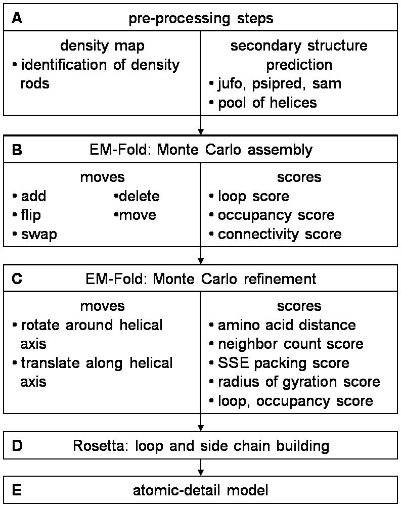
Flowchart of the entire protocol. A) Density rods are identified in a medium resolution density map. A pool of α-helices is built using secondary structure prediction algorithms. B) The assembly step of EM-Fold places α-helices from the pool into density rods. C) An EM-Fold refinement step improves the placement of α-helices within the density rods. D) Loops and side chains are built in Rosetta for the best of the refined EM-Fold models. E) One of the final full atom models is likely to be very close in RMSD to the native structure.

100% success rate for the perfect secondary structure prediction benchmark

In a first test 20,000 models were built for each of the ten benchmark proteins using the correct secondary structure. The Monte Carlo simulation was run until a total of 2,000 subsequent steps were rejected with no improvement in the overall score. The agreement with the density, which is simulated for the benchmark proteins, is assessed by a combined occupancy score (see Supplemental Figure 1), a loop score, and a connectivity score (see Supplemental Figure 2). A predicted fold is considered correct if all α-helices have been placed in the appropriate simulated density rods with the correct orientation of the α-helical axis. A high rank for the correct fold among the 20,000 models generated indicates success of the protocol.

The true model is found among the best 10 scoring models for all the benchmark cases (Table 1). In 50% of the cases the true model is ranked first. In the cases where the true model is not ranked first, the better ranking models are similar in topology to the true model and frequently only have a single α-helix or a pair of α-helices in an incorrect orientation. This demonstrates that the assembly step can clearly distinguish native-like from non-native models if the correct secondary structure is used as input. The RMSDs of the correct topology models range between 2.9 Å and 3.4 Å over the α-helical residues (Table 1).

Table 1.

Overview of the benchmark with ten α-helical proteins. Results are shown for both realistic secondary structure prediction, as well as for perfect secondary structure prediction in parentheses.

protein	rank assemblya	rmsd assembly [Å]b	rank refinementc	rmsd refinement [Å]d	rank loope	rmsd loop [Å]f	Helices in final partial modelg
1IE9	1 (1)	3.7 (3.3)	5 (1)	3.7 (2.6)	1 (1)	5.9 (7.8)	4 [4]
1N83	1 (1)	6.2 (3.2)	2 (1)	5.9 (2.4)	1 (7)	7.1 (3.7)	5 [5]
1OUV	6 (10)	3.0 (3.1)	4 (6)	2.9 (2.3)	1 (1)	4.3 (4.8)	9 [9]
1QKM	16 (1)	3.6 (3.1)	2 (1)	2.7 (3.3)	2 (7)	3.9 (4.2)	5 [5]
1TBF	100 (8)	3.1 (3.2)	20 (17)	2.8 (2.7)	1 (3)	4.1 (4.2)	12 [11]h
1V9M	− (1)	− (3.3)	− (1)	− (2.0)	− (2)	− (6.7)	7 [4]
1XQO	− (2)	− (3.3)	− (7)	− (2.1)	− (1)	− (5.0)	6 [2]
1Z1L	150 (3)	3.1 (3.4)	72 (13)	3.2 (2.5)	1 (1)	5.9 (5.5)	9 [9]
2AX6	1 (1)	4.0 (3.4)	5 (1)	3.2 (3.4)	3 (8)	6.6 (9.2)	5 [5]
2CWC	− (2)	− (2.9)	− (8)	− (2.4)	− (2)	− (7.1)	3 [0]
rhodopsin	2	3.4	1	3.1	1	7.9	-

^arank of true model after assembly step

^brmsd of backbone atoms in helices of true model after assembly step (compared to PDB coordinates)

^crank of true model after refinement step

^drmsd of backbone atoms in helices of true model after refinement step

^erank of true model after loop building step

^frmsd of all atoms in true model after loop building step

^gNumber of helices in final partial model based on 50% consensus placement; the number of correctly placed helices in these partial models is shown in square brackets. These results are also depicted in Figure 4.

^hThe one helix in the partial model of 1TBF that has not been correctly placed has been placed into the correct density rod, however with antiparallel orientation

For each of the ten proteins, the 50 best scoring models from the assembly step were refined. In this process a wider variety of types of scores (described in Materials and Methods) is used to evaluate the models. After refinement the RMSDs of the best scoring correct topology model range between 2.0 Å and 3.4 Å, again considering only the α-helical residues, and the true model is found among the best 17 scoring models (Table 1). These rankings are within the accuracy limit of the scoring functions.

Rosetta was used to build loops for the 20 best scoring models after the refinement run. The RMSD of the true model after loop building ranges between 3.7 and 9.2 Å (Table 1), which is an excellent level of agreement for de novo models considering the large size of the proteins. After the loop building step, all of the true models are ranked within the best 8 scoring topologies according to the Rosetta score. Thus, EM-Fold is able to identify the true topology within the top ten best scoring models built, given completely correct secondary structure information.

EM-Fold selects the best α-helices from a consensus pool generated from state-of-the art secondary structure predictions

A combination of three state-of-the art secondary structure prediction programs jufo (Meiler and Baker, 2003a; Meiler et al., 2001), psipred (Jones, 1999) and sam (Chandonia and Karplus, 1999; Karplus et al., 1997) was used to simulate a realistic prediction scenario. The utilization of different programs avoids usage of incorrect secondary structure if one of the methods fails. Wherever an α-helix is predicted with a probability of higher than 0.5 for more than nine subsequent residues, this α-helix is inserted into the pool of considered secondary structure elements. Smaller α-helices are ignored as these cannot be confidently identified in intermediate resolution density maps. Further, a consensus prediction (average of all three methods) and a consensus prediction where α-helices longer than 21 residues are broken into two smaller α-helices are included. Within the ten benchmark proteins there are 93 α-helices that have at least 12 residues. Each of these α-helices is identified by at least one secondary structure prediction technique, although the predicted lengths and confidence levels differ.

Secondary structure predictions tend to yield α-helices that are too short, thus three different pools (A, B and C) of secondary structure elements were tested including lengthened α-helices in pools B and C (see Materials and Methods). The best results for the assembly step are obtained with the most diverse pool of secondary structure elements (pool C), where the average deviation between predicted and correct α-helix length is only 0.4 residues per α-helix (Supplemental Table 2). This finding stresses two points: 1) The more accurate the secondary structure prediction is, the better the results of the assembly algorithm will be - a finding that is also supported by the benchmark test using the correct secondary structure information. 2) A larger pool, which includes many inaccurate secondary structure elements, does not negatively influence the success of the assembly protocol. In other words, the assembly protocol identifies and uses the best possible secondary structure elements available in the pool. Only pool C was used for the realistic secondary structure benchmark as it has been demonstrated to most accurately represent the secondary structure of the proteins.

De novo folding of α-helical benchmark proteins with realistic secondary structure predictions

In the initial assembly step (see Figure 1B) 60,000 models were built for each protein using the most diverse secondary structure pool (pool C). Building one model takes approximately 60s on a single JS20 IBM 2.2GHz PowerPC. The models were ranked by score (Table 1). Our results indicate that despite the inaccuracies of secondary structure prediction, after the assembly step the true model is found among the best 150 scoring models for seven out of the ten proteins. In particular for four of the benchmark proteins the true model is found among the best ten scoring models, and the average rank of the seven correct models is 39. The RMSD of the correct model after the assembly step ranges from 3.0 to 6.2 Å (Table 1). The best 150 models by score enter the refinement protocol without manual analysis.

After refinement (see Figure 1C) the ranking of the correct model improves to at least rank 72, for five of the benchmark cases it even improves to rank 5 or better. Further, the quality of the true model, as assessed by the RMSD, improves for five out of seven cases with a range over all seven proteins of 2.7 to 5.9 Å (Table 1). Supplemental Figure 3 illustrates the improvement of α-helix orientations during the refinement step for three examples. The best 75 models by score enter the loop building protocol without manual analysis.

Loops are built for the best 75 scoring models after refinement. For each of the 75 refined models 100 loop models are built using Rosetta. After ranking of these 7,500 models according to their Rosetta score, the true model is within the best three scoring models for all seven proteins (see Table 1). Even though the average rank of the correct model after the assembly step was only 39, the user only needs to consider the top three scoring models after loop building. The accuracy of these models is in the range of 3.9 to 7.1 Å (Table 1). This RMSD range is comparable to those built with correct secondary structure elements and acceptable considering the large size of the proteins. Superimpositions of the final Rosetta model with the native structure are shown for all seven proteins (Figure 2).

Figure 2.

Superimposition of the final models (colored in rainbow) of 1IE9 (A), 1N83 (B), 1OUV (C), 1TBF (D), 1Z1L (E), 1QKM (F) and 2AX6 (G) with the original PDB structures (grey). These proteins range in size from 255 to 345 residues. The displayed models have RMSDs ranging from 3.9 Å to 7.1 Å compared to the PDB structure. Regions that are only seen in the models (such as the N-terminus of 1TBF) correspond to parts of the protein that are missing in the PDB file. Panel H shows the model of rhodopsin after the loop building step (rainbow) in the experimental density model. The crystal structure of rhodopsin is shown in grey for comparison. The model and crystal structure have an RMSD of 7.9 Å. A blow-up of one Trp side chain and its corresponding density bump is shown. The Trp side chain of the crystal structure is shown in black for comparison. It is apparent that the Trp in the model was placed in the correct height of the density rod. The rotation of the α-helix in the model is off by about 150° however. This is not unexpected and could be corrected by a subsequent refinement protocol.

Consensus placement of α-helices correlates with correct positioning and can be used as a measure of confidence

In order to develop a measure that is independent of the score and that can evaluate the correctness of a particular model, the consensus placement of α-helices into specific density rods was analyzed. Models after the assembly step and after loop construction were evaluated. In both cases the benchmarks indicate that if a specific α-helix is found repeatedly in the same density rod within the set of best scoring models it was placed correctly. Receiver Operator Characteristic (ROC) curve representations for placement confidence after the assembly and loop building steps are shown in panels A and B of Figure 3. The total areas under the curve are 0.81 and 0.86 respectively, indicating strong correlations between frequent placement and correct positioning. For example, a placement of a particular α-helix into a specific density rod that is found in 70% of the top scoring models after the assembly step has a 71% confidence level of being correct. The results for models after the loop building step are even better, corroborating the ability of the algorithm to enrich for true-topology models. For example, a placement of a particular α-helix into a specific density rod that is found in 50% of the top scoring models after the loop building step has an 82% confidence level of being correct.

Figure 3.

ROC curves for the confidence in repeated placements as well as the performance of the connectivity score. A) ROC curve of the confidence in placements of single α-helices into density rods based on repeated placements after the assembly step. The fraction of correct placements (true positives / (true positives + false positives)) over the fraction of wrong placements (true negatives / (true negatives + false negatives)) is plotted. The connection between repetition rate and placement confidence has been added to the ROC curve. For example, a placement of a particular α-helix into a specific density rod that is found in 50% of the top scoring models after the assembly step has a 62% confidence of being correct. The area under the curve is 0.81 where 0.5 represents a random measure. B) ROC curve of the confidence in placements of single α-helices into density rods based on repeated placements after the loop building step. The fraction of correct placements (true positives / (true positives + false positives)) over the fraction of wrong placements (true negatives / (true negatives + false negatives)) is plotted. The connection between repetition rate and placement confidence has been added to the ROC curve. The steep increase at the beginning demonstrates that when the same α-helix is placed in one specific density rod in at least 60% of the cases, this placement is virtually always correct. The area under the curve is 0.93 where 0.5 represents a random measure. C) ROC curve of the connectivity score. The fraction of correct connections (true positives / (true positives + false positives)) over the fraction of wrong connections (true negatives / (true negatives + false negatives)) is plotted. The steep increase at the beginning demonstrates that the strongest correct connections score all better than any of the wrong connections. The area under the curve is 0.86 where 0.5 represents a random measure.

It would be desirable if the confidence measure allowed distinction between successful and unsuccessful cases in the benchmark. Partial models containing only the α-helices placed with a >50% repetition rate were built for all 10 benchmark proteins. A 50% cutoff ensures that no other placement into that density rod can occur more frequently. We evaluated the overall confidence in a model where k α-helices have been placed confidently out of a total of n α-helices by calculating the number of possibilities to place k α-helices into a total of n density rods (2^k*n!/(n−k)!). This equation explicitly takes into account the number of confidently placed α-helices (k) and the total number of α-helices in the protein (n), and implicitly the fraction of confidently placed α-helices. It also accounts for the fact that placing a specific fraction of α-helices confidently in a large protein is considerably less likely than placing the same fraction of α-helices confidently in a smaller protein. The results of this analysis are plotted in Figure 4. The overall confidence scores for the 10 benchmark proteins fall into two regions within this plot. Some proteins have a low number (3–7) and others have a high number (10–14) on this scale (separated by the dashed line in Figure 4). Proteins below the dashed line contain both successful and unsuccessful cases indicating that there is ambiguity for partial models in this range. However, proteins in the upper region (above the dashed line) contain only successful benchmark cases, suggesting that a high value on this overall confidence scale identifies correct topologies. Interestingly, the partial model that we built for adenovirus protein IIIa (discussed below) clusters with the benchmark proteins in the high range of this scale. This gives credence to the protein IIIa model in the absence of an atomic resolution structure.

Figure 4.

EM-Fold results for the 10 benchmark proteins and adenovirus protein IIIa evaluated on the basis of the number of confidently placed α-helices and the total number of α-helices in the protein. The y-axis represents the log base 10 of the number of possible topologies with k confidently placed α-helices in n density rods using the following equation (2^k*n!/(n−k)!). The length of each bar in the plot corresponds to the total number of α-helices in a protein (n). The sum of the black and gray squares within a bar represents the number of α-helices that were confidently placed by EM-Fold (i.e. with >50% repetition rate) (k). Within the subset of confidently placed α-helices, the correctly placed α-helices are in black. The ten benchmark proteins split into two groups as indicated by the dashed line: those with a low number (3–7) and those with a high number (10–14) on this scale. A high number indicates a low probability of confidently placing these α-helices by chance. While there are both successful and unsuccessful benchmark cases below the dashed line, only successful cases are found above the line. For adenovirus protein IIIa 11 out of 14 α-helices are confidently placed by EM-Fold (diagonal pattern, k) and the y-axis number is well above the dashed line.

Poor secondary structure prediction leads to poor assembly results

The three proteins that were not successfully assembled have the poorest secondary structure prediction with an average deviation of 0.8 residues per α-helix in Pool C, compared to an average deviation of 0.3 residues per α-helix for the remaining seven proteins (Supplemental Table 2). This underscores the fact that failure to find the true solution is not a shortcoming of the assembly algorithm but rather a result of sub-optimal secondary structure prediction. The correct solution of 2AX6 is found despite its poor secondary structure prediction (average deviation of 0.8 residues per α-helix in Pool C) because this protein is small with only six α-helices. In this case the assembly algorithm has to probe a considerably smaller search space and thus can overcome the limitation of poor secondary structure information.

Rosetta iterative high resolution refinement achieves accurate atomic-detail in parts of the protein models

One of the main challenges of computational protein structure prediction is recovering accurate atomic detail of interfaces within proteins. The top ten scoring loop models of all the seven proteins where the correct topology was identified after loop building were subjected to an iterative Rosetta refinement protocol (see Experimental Procedures). The objective of this protocol was to test the ability of the method to build accurate atomic-detail structural models at least in part of these proteins. Further it was investigated whether it is possible to uniquely identify the correct topology by the Rosetta energy score.

Figure 5 shows close-up views of three α-helix-helix interfaces in the best scoring correct topology model for 1QKM after iterative high resolution refinement. The protocol was able to recover native side chain packing in some of the α-helical interfaces (Figure 5, A and B). However, even in the best scoring model there are still interfaces that are not recovered (Figure 5, C). Supplemental Figure 4 shows the total full-atom Rosetta energy plotted versus the RMSD of the model for all of the proteins. While low RMSD models cannot be identified solely by energy, in six out of seven cases the correct topology can be identified by its enrichment in the 10% model with lowest energy (7.6 for 1Z1L, 4.0 for 1IE9, 3.8 for 1OUV, 2.6 for 1QKM, 1.6 for 1TBF and 1.2 for 1N83). We hypothesize that these enrichments are due to lower energy (higher quality) of the fraction of α-helical interfaces that were built accurately at atomic detail. At the same time non-native α-helix interfaces introduce a background noise that make the energy of models with correct topology often comparable to those of incorrect topology.

Figure 5.

A-helix-helix interfaces within the best scoring, correct topology, full atom model of protein 1QKM after ROSETTA iterative high resolution refinement. The full atom model is shown in rainbow colors, while the native PDB is depicted in grey. Panels A and B show examples of near-native interfaces in the final model. The α-helix orientations and positions have been correctly identified and the side chain conformations are generally close to the native PDB. Panel C shows an example of a α-helix-helix interface that could not be recovered.

For all seven proteins, the native structure obtained from the PDB was minimized in the refinement protocol as well (Supplemental Figure 4). Its energy is clearly lower than the energy of any of the models built. Thus the absence of models that have accurate atomic detail throughout the entire protein chain is a sampling rather than a scoring problem. This is expected for de novo protein models of 250 and more residues. The size of these systems far exceeds the 90 residue practical limit for de novo high-resolution structure prediction (Bradley et al., 2005). However, our finding of native-like α-helix interfaces in portions of these models is an encouraging result that suggests that all-atom accurate atomic-detail models can be achieved as cryoEM reaches higher resolution, and as computational techniques improve.

Comparison of EM-Fold with a computational prediction method for α-helical membrane proteins

In 2007, Kovacs et al. introduced a protocol for predicting atomic resolution details for α-helical membrane proteins guided by EM density maps (Kovacs et al., 2007). This method uses scripts within the internal coordinate mechanics (ICM) software environment. The ICM-based approach was demonstrated with simulated EM density maps at intermediate resolution for three membrane proteins (GpA, KcsA, MscL). ICM-based flexible fitting of α-helices, optimization of sidechain conformations, and refinement of atomic models resulted in impressive final RMSDs between 0.9 and 1.9 Å for the three test membrane proteins.

While the general idea of guiding protein structure prediction by α-helical density rods observed in intermediate resolution EM density maps is the same for the ICM-based method (Kovacs et al., 2007) and EM-Fold, there are substantial differences between the methods. In the demonstration of the ICM approach perfect secondary structure prediction was assumed. We have tested EM-Fold with both perfect and realistic secondary structure prediction information including variations in α-helix lengths. Secondly, the test proteins used in the ICM demonstration are sufficiently small (with 1 or 2 α-helices per monomer), and have α-helices of differing lengths (in the case of 2 α-helices per monomer), so that the assignment of α-helices into specific density rods is trivial. The centerpiece of the EM-Fold protocol is the assembly step (Figure 1B), which is designed to identify the topology of a protein from its α-helical secondary structure prediction and the positions of density rods in the density map. Subsequent steps (Figure 1C and D) refine the model. The ICM-based algorithm does not have an assembly step, while the refinement steps in both protocols follow similar principles. In their current setups these algorithms are complementary and it is conceivable that models derived from EM-Fold could be input into ICM for further refinement.

Benchmark of EM-Fold on experimental bovine metarhodopsin density map

To demonstrate EM-Fold’s ability to work reliably in conjunction with experimental data, we built a model for bovine metarhodopsin based on the 5.5 Å resolution cryoEM density map obtained from the EMDB Database (Ruprecht et al., 2004). The crystal structure of bovine rhodopsin (PDBID 1GZM, (Li et al., 2004)) was used to evaluate the results. The crystal structure is in a different conformational state than the cryoEM structure. The overall fold of the protein is the same however as the authors note that the meta I formation involves no large movements or rotations of α-helices from their ground state (Ruprecht et al., 2004). So while there may be structural differences in the loop regions, the α-helical regions that are modeled in the protocol are well described by the crystal structure. Interestingly the authors report density bumps for several Trp side chains in the 5.5 Å resolution cryoEM density map. Bovine rhodopsin is mostly α-helical (63%) and slightly larger than the largest of the 10 benchmark proteins (349 residues, Supplemental Table 1).

The same protocol that was used for the ten benchmark proteins was applied to bovine metarhodopsin. The results are summarized in Table 1. The correct topology is ranked second after the assembly step and is ranked first after the refinement step. After the loop building step the correct topology is the best scoring model. This model has an RMSD of 7.9 Å to the crystal structure. If the crystal structure was not available, we could evaluate the EM-Fold results on the basis of the overlap between Trp sidechains and Trp density bumps on rods. Only a single good scoring model has all of the Trp containing α-helices in density rods with Trp density bumps. This model corresponds to the correct topology. These results demonstrate the ability of EM-Fold to work accurately in combination with experimental density maps. The rather large RMSD value is in part caused by the conformational change between crystal and cryoEM structure, particularly in the loop regions. The RMSD over α-helical residues is only 3.1 Å, making this an excellent model for a protein of this size.

Evaluation of adenovirus protein IIIa folds by EM-Fold

We have also applied EM-Fold to the medium resolution cryoEM density assigned to protein IIIa in the adenovirus capsid (Saban et al., 2006). In this case we do not have an atomic resolution structure for protein IIIa. This is a challenging case for EM-Fold because the α-helical region of protein IIIa is larger than any of the benchmark proteins and it has a two-lobe topology (Figure 6). This two-lobe density region contains 14 manually identified density rods and is assigned to the N-terminal 400 residues of protein IIIa, which are predicted to be highly α-helical. As none of the 10 benchmark proteins or rhodopsin have a two-lobe topology, this complication has not been tested in EM-Fold. Therefore we used experimental information to assign the two lobes and also to filter the models produced by EM-Fold.

Figure 6.

Experimental cryoelectron microscopy (cryoEM) density map of adenovirus protein IIIa (grey) shown segmented from an adenovirus reconstruction at 6.9 Å resolution (FSC 0.5 threshold) (Saban et al., 2006). 14 rods of minimum length 18 Å have been identified as α-helical regions (red). Each rod is labelled with a letter and the number of α-helical residues corresponding to its length. The EM-Fold assembly step involves placing α-helices from the secondary structure prediction pool into the 14 identified density rods. The protein IIIa density has a two-lobe topology, with Lobe 1 comprised of rods A-G and Lobe 2 comprised of rods H-N. In the adenovirus capsid, Lobe 1 is closer to the penton base.

In order to extend the resolution of the Ad35F cryoEM structure, we increased the dataset size to a total of 7133 particle images and performed several additional rounds of Frealign refinement. The final Ad35F structure is based on 3040 particle images and has a resolution of 6.8 Å at the FSC 0.5 threshold (and 5.8 Å at the FSC 0.3, and 5.2 Å at the FSC 0.143 thresholds). A plot of the FSC for the refined map can be seen in Supplemental Figure 5. The crystal structure of the Ad5 hexon reveals that there are two α-helices of ten or more residues that have a Trp (Rux et al., 2003). We observe prominent bumps for the Trp side chains on each of these two α-helices in the 6.8Å cryoEM density map (see Supplemental Figure 6).

Using the criteria developed to identify Trp in hexon, three possible positions (in rods E, K, L) were identified in the protein IIIa that might correspond to a Trp side chain. The side chain bump in rod E is at the end of the rod, while the bumps in rods K and L are both in the middle of the rods and in fact form a connection between these two rods. Analysis of the protein IIIa sequence indicates that there is only one Trp in a predicted α-helix (residue 27) and that it corresponds to the first or second residue in the predicted α-helix. This excludes rods K and L, as corresponding to the α-helix with a Trp, since the observed bumps are in the middle of these rods. We hypothesize that the observed bumps in rods K and L belong to two aromatic side chains that are in contact. After analyzing the cryoEM density, we conclude that the most likely rod to contain the predicted α-helix with a Trp (amino acids 27–39) is rod E.

This lobe assignment for protein IIIa is in agreement with the N-terminal tagging experiment recently published (San Martin et al., 2008). The protein IIIa peptide tag study localizes the N-terminus of protein IIIa to the inner capsid surface close to the interface between penton base and the peripentonal hexons. Specifically the difference density attributed to an N-terminal FLAG tag on protein IIIa is observed in the vicinity of what we refer to as rod E in lobe 1 of protein IIIa (Figure 6). Therefore both the analysis of the sidechain density and the protein IIIa N-terminal tagging information indicate that lobe 1 should be assigned to the most N-terminal portion of protein IIIa.

After applying the same EM-Fold protocol used for the ten benchmark proteins and rhodopsin, we analyzed the top 100 models for protein IIIa and found that 33 of these have the N-terminal ~200 residues of protein IIIa positioned into lobe 1. A detailed analysis of this subset of models indicates that 14 models have the predicted α-helix for residues 27–39, which includes the Trp at position 27, placed into rod E. We consider these 14 selected models the most likely models for protein IIIa. Within these 14 models, we note that four α-helices (corresponding to residues 50–60, 70–83, 230–242 and 251–264) are placed into specific rods (G, B, H and J, respectively) in all of the cases. Therefore we assign these α-helices, as well as the Trp-containing α-helix (rod E), as having a very high (>94%) confidence level. An additional six α-helices are placed with >50% repetition rate and thus are assigned a high (>82%) confidence level as labeled in the ROC curve in Figure 3B. A partial model of protein IIIa that contains these 11 confidently placed α-helices is shown in rainbow in Figure 7, panels A and B. The remaining three α-helices are shown in grey and the loop regions are shown in white indicating that their positioning within the density is more ambiguous. The number of confidently placed α-helices puts this partial model into the confident region in Figure 4, further increasing the probability that it is correct. The proposed 50% confidence protein IIIa model is shown in context with penton base and two nearby peripentonal hexons (Figure 7C). Also, the agreement of the Trp (residue 27) side chain with the bump in rod E is shown in Figure 7, panel D. Interestingly, one of the α-helices placed with a high confidence level (rod L) contains a Tyr residue (Y369) in the middle of the α-helix that corresponds to the density connection observed between rods K and L. On top of this another confidently placed α-helix places Y299 in the middle of the connected density rod (rod K). This confidence assignment agrees perfectly with the observed density connection between rods K and L and gives further credence to our model. We anticipate that higher resolution cryoEM density revealing more of the side chains, combined with additional computational modeling, would resolve the remaining ambiguities in the protein IIIa fold model.

Figure 7.

Model of protein IIIa. A) A reduced model of protein IIIa where only α-helices that have been placed with at least 50% repetition rate are colored in rainbow. This topology agrees with the San Martin et al. (San Martin et al., 2008) results. 11 out of 14 α-helices can be placed with a confidence of at least 82%. The remaining three α-helices have been colored in grey while the loop regions are shown in white. B) Same as in A, but shown but shown in density. E) Side view of partial model of protein IIIa (rainbow) in contact with penton base (yellow) and two peripentonal hexons (light blue). F) Density bump in rod E of the refined Ad35F density of protein IIIa that has been assigned to Trp27. The arrow marks the position of the side chain.

Conclusions

EM-Fold is a novel computational protein folding algorithm that assembles α-helical proteins guided by medium resolution density maps. In a later stage EM-Fold can be extended to include β-strands in the assembly algorithm once more cryoEM density maps allow an unambiguous identification of β-strands. For future applications manual identification of density rods will be replaced by an in-house algorithm that is currently under development. A benchmark on ten proteins shows a 100% success rate for the assembly of α-helices when the correct secondary structure information is assumed. When predicted secondary structure information is used, which includes some incorrect information, the success rate drops to seven out of ten. Our results demonstrate that the 30% failure rate is linked to incorrect secondary structure prediction information and future developments will include improving the secondary structure prediction input. This might be done by either improving the secondary structure prediction algorithms themselves or – as demonstrated here – by including more diverse predictions into a more complex pool of α-helices prior to assembly. The final models generated by EM-Fold display RMSDs in the range of 3.9 Å to 7.1 Å for the benchmark proteins. A complete model for rhodopsin with 7.9 Å RMSD could be built based on an experimental density map. These results demonstrate that de novo protein structure prediction can be extended to proteins well beyond 150 amino acids if the search is guided by medium resolution density maps.

The iterative Rosetta refinement protocol did not completely succeed in refining the models to accurate atomic detail. Given the large size of the proteins this is not entirely surprising. However, portions of the final models, including specific α-helix-helix interfaces, do have correct atomic resolution detail. These partial native-like arrangements lead to an enrichment of correct topology models by energy. An improved iterative sampling protocol that includes the density map as an experimental restraint might allow refinement to atomic detail accuracy for complete models in the future.

EM-Fold has been applied to build a model of adenovirus protein IIIa, a protein for which we have a medium resolution cryoEM density map but no atomic resolution structure. Based on the experimental constraints provided by N-terminal tagging (San Martin et al., 2008) as well as observed side chain density in a refined cryoEM density map, we were able to assign the lobe topology of the protein. We also used this experimental information as a filter to select the most likely fold models for protein IIIa produced by EM-Fold. We present a fold model for protein IIIa with 11 of the 14 α-helices placed with a high level of confidence. Future improvements to the EM-Fold method will include improving secondary structure prediction, consideration of large sidechain information during the assembly stage, and simultaneous assembly of α-helices and β-strands.

Experimental Procedures

Overall protocol

The flowchart of the full assembly process is shown in Figure 1. The generation of a pool and identification of density rods is followed by the main assembly step in EM-Fold, a refinement step within EM-Fold, and loop and side chain building in Rosetta. The assembly step builds α-helices from the pool into the density rods. Three sequence-independent, computationally inexpensive, and therefore low resolution scores are used to build a large number of initial models. The best scoring models from the assembly step are refined using sequence-dependent, medium-resolution scores and leaving the overall fold of the protein unchanged. The last step of the assembly protocol uses the existing Rosetta software (Rohl et al., 2004a; Sood and Baker, 2006) to model loops for the best-scoring models that emerged from the refinement step. Side chains are constructed using Rosetta relaxation and repacking strategies (Bradley et al., 2005). This is the computationally most expensive and highest resolution step of the model building process and is thus only applied to a handful of final models.

Secondary structure prediction pool

To minimize secondary structure prediction inaccuracies, three different secondary structure pools (A, B, C) were investigated. Pool A uses the secondary structure prediction programs jufo (Meiler and Baker, 2003a; Meiler et al., 2001), psipred (Jones, 1999) and sam (Chandonia and Karplus, 1999; Karplus et al., 1997) to get three state predictions of the secondary structure of the benchmark cases. Sequences of more than nine amino acids predicted to be α-helical were considered to be a likely position of a non-short α-helix and were added to a “pool” of possible secondary structure elements. In addition to the individual predictions, a consensus secondary structure prediction was calculated by averaging jufo, sam, and psipred. Also α-helices longer than 21 residues were split into, two further expanding this pool.

In pool B copies of the α-helices from pool A were replaced with copies that are extended by one amino acid on both sides. Thus pool B has the same size as pool A, but all of the α-helices are two residues longer. This procedure eliminated the bias in pool A towards α-helices that are too short and reduces the per α-helix deviation from the correct secondary structure from 1.5 residues in pool A to 0.8 residues in pool B.

Pool C combines pools A and B and adds further versions of α-helices extended by one amino acid either on the N-terminus or the C-terminus. As a result the secondary structure element pool C has four versions of each α-helix with different lengths available for assembly. The per α-helix deviation from the correct secondary structure in pool C is 0.4 residues. The length deviations of the elements that are closest in length and have maximal sequence overlap with the true α-helices are reported in Supplemental Table 2 for all three versions of the prediction pool.

EM-Fold scoring function

Three sequence-independent scores are used during the assembly of the fold: a loop, an occupancy, and a connectivity score. The loop score is a knowledge-based score that evaluates the likeliness of a certain C_α-C_α distance between terminal residues in an α-helix being bridged by a specific number of residues. It has a preference for short Euclidean distances between beginning and end of a loop (data not shown).

The occupancy score evaluates the length agreement of a density with an α-helix that is placed in it (see Supplemental Figure 1) with unfilled densities getting the maximum unfavorable score. Thus the occupancy score drives the algorithm toward filling the density map completely.

The connectivity score is based on the assumption that for short loops a medium resolution density map contains valuable information in the form of stronger density in the loop regions between density rods. The connectivity score employs a skeletonization algorithm (Ju et al., 2007) to find the highest intensity connection between all pairs of termini of density rods that are closer than 10 Å in space. This information is converted into a score that assesses whether the connection is a strong or a weak one (see Supplemental Figure 2).

The connectivity score has been tested on the ten benchmark proteins. Within the ten proteins there are 65 pairs of density rods whose ends are closer than 10 Å. 25 of these pairs correspond to connected density rods. Figure 3C shows a ROC curve based on the strength of the connection. The area under the curve is 0.86, clearly showing the ability of the connectivity score to enrich for native connections. Out of 14 connections whose strength is more than one standard deviation above the average connection strength, 12 correspond to true connections.

EM-Fold assembly step

The sampling of conformational space is performed in a Monte Carlo algorithm in conjunction with the Metropolis criterion. When placing an α-helix from the pool into a density two physical constraints are checked: First, whether the length of the α-helix fits the density within a deviation of three residues (corresponding to a maximum length deviation of 4.5 Å). This “length-tolerance-check” accounts for inaccuracies both in secondary structure prediction and in length determination of density rods. Secondly, it is checked whether the residues between the α-helix and all previously placed α-helices are sufficient to fill the gaps between α-helices. The maximum loop length was set to 3.0 Å per amino acid plus an additional 6.0 Å per loop. If one of the constraints is violated, the move will be rejected because the resulting model would not agree with the density map. All placements that do not violate these constraints are evaluated by the three sequence-independent scores discussed above. Assuming that x density rods have been identified in the density map and the pool contains y α-helices, there is a total of N_pos number of possibilities to place the α-helices into the density rods.

$$N_{\text{pos}}=\left(\begin{array}{c}n\\ k\end{array}\right)k!2^k=\frac{n!}{(n-k)!}{2}^k,$$

with n=max(x;y) and k=min(x;y). This same equation is also used to calculate an overall confidence score for a partial model built by EM-Fold by reassigning n to the total number of α-helices and k to the number of confidently placed α-helices (with >50% repetition rate).

The Monte Carlo moves (see Figure 8) that are used in the assembly step are: B) adding an α-helix from the pool to the model, C) deleting an α-helix from the model, D) flipping the orientation of an α-helix in the model, E) swapping the positions of two α-helices within the model, F) swapping an α-helix from the model with one from the pool, and G) moving an α-helix from the model to an empty density rod. The orientation of an α-helix after any move that results in placement of a new α-helix (moves B, E, F, and G) is arbitrary. A simulated annealing Monte Carlo Metropolis search is used where the temperature is decreased linearly from 0.25 to 0.08 over 2000 rejected steps. The weights of the scores are 1.0 (loop), 0.4 (occupancy) and 0.8 (connectivity). The final total scores range from −4.2 (2AX6) to −22.1 (1OUV). It is important to note that the temperature values are somewhat arbitrary and do not correspond to physiologically relevant temperatures.

Figure 8.

Schematic representation of the moves used in the assembly step of the protocol. Panel A shows the state of the model before the move. The add move (B) adds an α-helix from the pool into an empty density rod. The delete move (C) removes an α-helix from a density rod and returns it to the pool. The flip move (D) rotates one α-helix within a density rod by 180° perpendicular to its long axis. The swap move (E) exchanges two α-helices within density rods. The swap with pool move (F) exchanges an α-helix within a density rod with one from the pool. Move G removes an α-helix from its density rod and places it into another empty density rod.

EM-Fold refinement step

The lowest scoring models are used in a second medium resolution Monte Carlo refinement search. This refinement step uses different moves and scores than the previous assembly step. The moves constitute small perturbations of the model – shifts along the α-helical axis and rotations around the α-helical axis. A set of knowledge-based scores is used including an aminoacid-distance score, a neighbor-count score, a secondary-structure-element-packing score, a compactness-measure in form of a radius-of-gyration score, and the loop and occupancy scores already used in the previous step. These scores are described in detail in the supplementary data. The occupancy score avoids α-helices sliding out of their density rods. This refinement step maintains the fold of the model but identifies correct α-helix-helix-interfaces. A simulated annealing Monte Carlo Metropolis search is used where the temperature is decreased linearly from 0.25 to 0.03 over 2000 rejected steps. The weights of the scores are 10 (loop), 4 (occupancy), 0.2 (aadist), 0.2 (neighbor count), 0.14 (radius of gyration) and 2 (ssepack). The final total scores range from −139 (2AX6) to −367 (1TBF).

Rosetta loop and side chain building step

For identification of the correct fold as well as for building a full atom model of the protein the Rosetta software (Bradley et al., 2005; Rohl et al., 2004a; Sood and Baker, 2006) was used. The backbone atoms of the residues that are missing in the EM-Fold models are built using the Rosetta cyclic coordinate descent loop building protocol (Rohl et al., 2004a). The resulting models with loops are scored in the Rosetta force field and sorted according to their score. This score can discriminate the correct from non-native topologies as demonstrated in the benchmark. For the seven successful benchmark proteins the ten best scoring topologies according to the Rosetta score were chosen and underwent an extensive refinement protocol within Rosetta. This protocol included building 1,000 EM-Fold-refined models per topology (10,000 models total). For each of the 10,000 refined models, 5 loop models were built in Rosetta (50,000 models total).

Eight rounds of iterative side chain repacking and backbone relaxation in Rosetta followed (Bradley et al., 2005). All 50,000 models undergo round one. Only models that stay within 2.5 Å of the starting structure and are within the best 10 % scoring models according to the Rosetta full atom energy are run through rounds 2–8. After the eighth round the best 10 % scoring models are analyzed according to their enrichment for the correct topology. The enrichment is computed as the ratio of relative frequency of correct topology models within the best 10 % scoring models to relative frequency of correct topology models within all models.

Benchmark on simulated density maps

The proposed EM-Fold search algorithm was benchmarked on ten proteins that were chosen to be mainly α-helical, exhibit non-redundant folds, possess 250 to 350 residues and form 6 to 14 α-helices of at least 12 residues in length (Supplemental Table 1). Electron density maps for all ten benchmark cases were created from the coordinates. PDB2VOL of the Situs package (Wriggers and Birmanns, 2001) was used to simulate density maps with 6.9 Å resolution, a voxel spacing of 1.5 Å and Gaussian flattening. Positions and lengths of the density rods were identified manually since available α-helix identification algorithms did not perform satisfactorily for either the simulated densities of the benchmark proteins or for the protein IIIa density. Errors in manual identification of α-helix length can be compensated by the length tolerance that is used in the assembly step. To test the influence of the resolution of the simulated medium resolution density map, maps at 9.0 Å resolution were also simulated. Positions and lengths of the density rods were identified manually for the 9.0 Å resolution maps as well.

Furthermore, it should be stressed that, independent of whether the density rods are identified manually or using automated software, there is always the possibility that density regions in medium resolution density maps that do not correspond to α-helices are identified as α-helical regions. An example for this is a β-hairpin of at least 4 residues in each strand. Likewise it is possible that an α-helical region in the protein is not identified as a density rod in the map (in the case of a more flexible α-helix for instance). In both cases EM-Fold is still capable of finding the correct topology, as the algorithm neither requires all identified rods to be filled with α-helices, nor all predicted α-helices to be placed in identified rods.

Benchmark on experimental density map

EM-Fold was also benchmarked on the experimental cryoEM density map of bovine metarhodopsin (EMDB Entry EMD-1079). The density map is reported to have a resolution of 5.5 Å and has a voxel size of (0.4 Å, 0.5 Å, 1.7 Å). A single subunit of the protein was segmented from the density map. Bovine rhodopsin has 349 residues and is highly α-helical (63% α-helical) with 8 α-helices of 12 or more residues.

Protein IIIa structure elucidation

The adenovirus vector Ad35F was used in previous cryoEM structural studies (Saban et al., 2006) and has been refined further with more data (7133 particle images) with the program Frealign (Grigorieff, 2007). A negative temperature factor of 450Ų was applied to the final map and the structure was filtered at 5.1 Å using a filter with a cosine-shaped cut-off and a width of ~20 Fourier pixels. Ad35F is composed of the Ad5 capsid and the Ad35 fiber. The density for one copy of protein IIIa was segmented from an Ad35F reconstruction. The Ad5 protein IIIa has 585 residues. The 400 N-terminal residues are predicted to be mainly α-helical, while the remaining C-terminal residues are not predicted to have many secondary structural elements. In the density map 14 density rods of at least 18 Å in length and 6–7 Å diameter (corresponding to α-helices of at least 12 residues) were identified manually (Figure 6). A secondary structure element pool with a total of 257 α-helices was built using the protocol described for pool (C). 100,000 models were built for protein IIIa according to the assembly procedure established for the benchmark set of proteins. The models were ranked by score. 100 refined models were constructed for each of the top 150 models produced by the assembly step. The resulting 15,000 models were sorted by score and the top scoring model of each of the 150 topologies was selected for loop construction. A topological model built using EM-Fold is presented for the first 400 residues of protein IIIa.

EM-Fold availability

EM-Fold is freely available for academic use. It will be made available as a part of the Biochemical Library (BCL) that is currently being developed in the Meiler laboratory (www.meilerlab.org). In the meantime an executable can be obtained by contacting the authors.

References

- Alexander N, Bortolus M, Al-Mestarihi A, McHaourab H, Meiler J. De novo high-resolution protein structure determination from sparse spin-labeling EPR data. Structure. 2008;16:181–195. doi: 10.1016/j.str.2007.11.015. [DOI] [PMC free article] [PubMed] [Google Scholar]
- Baker ML, Jiang W, Wedemeyer WJ, Rixon FJ, Baker D, Chiu W. Ab initio modeling of the herpesvirus VP26 core domain assessed by CryoEM density. PLoS Comput Biol. 2006;2:e146. doi: 10.1371/journal.pcbi.0020146. [DOI] [PMC free article] [PubMed] [Google Scholar]
- Baker ML, Ju T, Chiu W. Identification of secondary structure elements in intermediate-resolution density maps. Structure. 2007;15:7–19. doi: 10.1016/j.str.2006.11.008. [DOI] [PMC free article] [PubMed] [Google Scholar]
- Bonneau R, Ruczinski I, Tsai J, Baker D. Contact order and ab initio protein structure prediction. Protein Sci. 2002a;11:1937–1944. doi: 10.1110/ps.3790102. [DOI] [PMC free article] [PubMed] [Google Scholar]
- Bonneau R, Strauss CE, Rohl CA, Chivian D, Bradley P, Malmstrom L, Robertson T, Baker D. De novo prediction of three-dimensional structures for major protein families. J Mol Biol. 2002b;322:65–78. doi: 10.1016/s0022-2836(02)00698-8. [DOI] [PubMed] [Google Scholar]
- Booth CR, Jiang W, Baker ML, Zhou ZH, Ludtke SJ, Chiu W. A 9 angstrom single particle reconstruction from CCD captured images on a 200 kV electron cryomicroscope. Journal of Structural Biology. 2004;147:116–127. doi: 10.1016/j.jsb.2004.02.004. [DOI] [PubMed] [Google Scholar]
- Bottcher B, Wynne SA, Crowther RA. Determination of the fold of the core protein of hepatitis B virus by electron cryomicroscopy. Nature. 1997;386:88–91. doi: 10.1038/386088a0. [DOI] [PubMed] [Google Scholar]
- Bowers PM, Strauss CE, Baker D. De novo protein structure determination using sparse NMR data. J Biomol NMR. 2000;18:311–318. doi: 10.1023/a:1026744431105. [DOI] [PubMed] [Google Scholar]
- Bradley P, Misura KM, Baker D. Toward high-resolution de novo structure prediction for small proteins. Science. 2005;309:1868–1871. doi: 10.1126/science.1113801. [DOI] [PubMed] [Google Scholar]
- Chandonia JM, Karplus M. New methods for accurate prediction of protein secondary structure. Proteins. 1999;35:293–306. [PubMed] [Google Scholar]
- Conway JF, Cheng N, Zlotnick A, Wingfield PT, Stahl SJ, Steven AC. Visualization of a 4-helix bundle in the hepatitis B virus capsid by cryo-electron microscopy. Nature. 1997;386:91–94. doi: 10.1038/386091a0. [DOI] [PubMed] [Google Scholar]
- Dal Palu A, He J, Pontelli E, Lu Y. Identification of alpha-helices from low resolution protein density maps. Comput Syst Bioinformatics Conf. 2006:89–98. [PubMed] [Google Scholar]
- Grigorieff N. FREALIGN: High-resolution refinement of single particle structures. Journal of Structural Biology. 2007;157:117–125. doi: 10.1016/j.jsb.2006.05.004. [DOI] [PubMed] [Google Scholar]
- Hanson SM, Dawson ES, Francis DJ, Van Eps N, Klug CS, Hubbell WL, Meiler J, Gurevich VV. A model for the solution structure of the rod arrestin tetramer. Structure. 2008;16:924–934. doi: 10.1016/j.str.2008.03.006. [DOI] [PMC free article] [PubMed] [Google Scholar]
- Jiang W, Baker ML, Jakana J, Weigele PR, King J, Chiu W. Backbone structure of the infectious epsilon 15 virus capsid revealed by electron cryomicroscopy. Nature. 2008;451:1130–U1112. doi: 10.1038/nature06665. [DOI] [PubMed] [Google Scholar]
- Jiang W, Baker ML, Ludtke SJ, Chiu W. Bridging the information gap: Computational tools for intermediate resolution structure interpretation. Journal of Molecular Biology. 2001;308:1033–1044. doi: 10.1006/jmbi.2001.4633. [DOI] [PubMed] [Google Scholar]
- Jones DT. Protein secondary structure prediction based on position-specific scoring matrices. Journal of Molecular Biology. 1999;292:195–202. doi: 10.1006/jmbi.1999.3091. [DOI] [PubMed] [Google Scholar]
- Ju T, Baker ML, Chiu W. Computing a family of skeletons of volumetric models for shape description. Comput Aided Des. 2007;39:352–360. doi: 10.1016/j.cad.2007.02.006. [DOI] [PMC free article] [PubMed] [Google Scholar]
- Karplus K, Sjolander K, Barrett C, Cline M, Haussler D, Hughey R, Holm L, Sander C. Predicting protein structure using hidden Markov models. Proteins-Structure Function and Genetics. 1997:134–139. doi: 10.1002/(sici)1097-0134(1997)1+<134::aid-prot18>3.3.co;2-q. [DOI] [PubMed] [Google Scholar]
- Kovacs JA, Yeager M, Abagyan R. Computational prediction of atomic structures of helical membrane proteins aided by EM maps. Biophys J. 2007;93:1950–1959. doi: 10.1529/biophysj.106.102137. [DOI] [PMC free article] [PubMed] [Google Scholar]
- Li J, Edwards PC, Burghammer M, Villa C, Schertler GF. Structure of bovine rhodopsin in a trigonal crystal form. J Mol Biol. 2004;343:1409–1438. doi: 10.1016/j.jmb.2004.08.090. [DOI] [PubMed] [Google Scholar]
- Lindert S, Stewart PL, Meiler J. Hybrid approaches: applying computational methods in cryo-electron microscopy. Curr Opin Struct Biol. 2009 doi: 10.1016/j.sbi.2009.02.010. [DOI] [PMC free article] [PubMed] [Google Scholar]
- Ludtke SJ, Baker ML, Chen DH, Song JL, Chuang DT, Chiu W. De novo backbone trace of GroEL from single particle electron cryomicroscopy. Structure. 2008;16:441–448. doi: 10.1016/j.str.2008.02.007. [DOI] [PubMed] [Google Scholar]
- Martin AG, Depoix F, Stohr M, Meissner U, Hagner-Holler S, Hammouti K, Burmester T, Heyd J, Wriggers W, Markl J. Limulus polyphemus hemocyanin: 10 angstrom cryo-EM structure, sequence analysis, molecular modelling and rigid-body fitting reveal the interfaces between the eight hexamers. Journal of Molecular Biology. 2007;366:1332–1350. doi: 10.1016/j.jmb.2006.11.075. [DOI] [PubMed] [Google Scholar]
- Meiler J, Baker D. Coupled prediction of protein secondary and tertiary structure. Proceedings of the National Academy of Sciences of the United States of America. 2003a;100:12105–12110. doi: 10.1073/pnas.1831973100. [DOI] [PMC free article] [PubMed] [Google Scholar]
- Meiler J, Baker D. Rapid protein fold determination using unassigned NMR data. Proc Natl Acad Sci U S A. 2003b;100:15404–15409. doi: 10.1073/pnas.2434121100. [DOI] [PMC free article] [PubMed] [Google Scholar]
- Meiler J, Baker D. The fumarate sensor DcuS: progress in rapid protein fold elucidation by combining protein structure prediction methods with NMR spectroscopy. J Magn Reson. 2005;173:310–316. doi: 10.1016/j.jmr.2004.11.031. [DOI] [PubMed] [Google Scholar]
- Meiler J, Muller M, Zeidler A, Schmaschke F. Generation and evaluation of dimension-reduced amino acid parameter representations by artificial neural networks. Journal of Molecular Modeling. 2001;7:360–369. [Google Scholar]
- Min GW, Wang HB, Sun TT, Kong XP. Structural basis for tetraspanin functions as revealed by the cryo-EM structure of uroplakin complexes at 6-A resolution. Journal of Cell Biology. 2006;173:975–983. doi: 10.1083/jcb.200602086. [DOI] [PMC free article] [PubMed] [Google Scholar]
- Misura KM, Baker D. Progress and challenges in high-resolution refinement of protein structure models. Proteins. 2005;59:15–29. doi: 10.1002/prot.20376. [DOI] [PubMed] [Google Scholar]
- Misura KM, Chivian D, Rohl CA, Kim DE, Baker D. Physically realistic homology models built with ROSETTA can be more accurate than their templates. Proc Natl Acad Sci U S A. 2006;103:5361–5366. doi: 10.1073/pnas.0509355103. [DOI] [PMC free article] [PubMed] [Google Scholar]
- Moult J. A decade of CASP: progress, bottlenecks and prognosis in protein structure prediction. Curr Opin Struct Biol. 2005;15:285–289. doi: 10.1016/j.sbi.2005.05.011. [DOI] [PubMed] [Google Scholar]
- Qian B, Raman S, Das R, Bradley P, McCoy AJ, Read RJ, Baker D. High-resolution structure prediction and the crystallographic phase problem. Nature. 2007;450:259–264. doi: 10.1038/nature06249. [DOI] [PMC free article] [PubMed] [Google Scholar]
- Rohl CA, Baker D. De novo determination of protein backbone structure from residual dipolar couplings using Rosetta. J Am Chem Soc. 2002;124:2723–2729. doi: 10.1021/ja016880e. [DOI] [PubMed] [Google Scholar]
- Rohl CA, Strauss CE, Chivian D, Baker D. Modeling structurally variable regions in homologous proteins with rosetta. Proteins. 2004a;55:656–677. doi: 10.1002/prot.10629. [DOI] [PubMed] [Google Scholar]
- Rohl CA, Strauss CE, Misura KM, Baker D. Protein structure prediction using Rosetta. Methods Enzymol. 2004b;383:66–93. doi: 10.1016/S0076-6879(04)83004-0. [DOI] [PubMed] [Google Scholar]
- Rossmann MG. Fitting atomic models into electron-microscopy maps. Acta Crystallographica Section D-Biological Crystallography. 2000;56:1341–1349. doi: 10.1107/s0907444900009562. [DOI] [PubMed] [Google Scholar]
- Ruprecht JJ, Mielke T, Vogel R, Villa C, Schertler GF. Electron crystallography reveals the structure of metarhodopsin I. EMBO J. 2004;23:3609–3620. doi: 10.1038/sj.emboj.7600374. [DOI] [PMC free article] [PubMed] [Google Scholar]
- Rux JJ, Kuser PR, Burnett RM. Structural and phylogenetic analysis of adenovirus hexons by use of high-resolution x-ray crystallographic, molecular modeling, and sequence-based methods. J Virol. 2003;77:9553–9566. doi: 10.1128/JVI.77.17.9553-9566.2003. [DOI] [PMC free article] [PubMed] [Google Scholar]
- Saban SD, Silvestry M, Nemerow GR, Stewart PL. Visualization of alpha-helices in a 6-angstrom resolution cryoelectron microscopy structure of adenovirus allows refinement of capsid protein assignments. J Virol. 2006;80:12049–12059. doi: 10.1128/JVI.01652-06. [DOI] [PMC free article] [PubMed] [Google Scholar]
- San Martin C, Glasgow JN, Borovjagin A, Beatty MS, Kashentseva EA, Curiel DT, Marabini R, Dmitriev IP. Localization of the N-terminus of minor coat protein IIIa in the adenovirus capsid. J Mol Biol. 2008;383:923–934. doi: 10.1016/j.jmb.2008.08.054. [DOI] [PMC free article] [PubMed] [Google Scholar]
- Schueler-Furman O, Wang C, Bradley P, Misura K, Baker D. Progress in modeling of protein structures and interactions. Science. 2005;310:638–642. doi: 10.1126/science.1112160. [DOI] [PubMed] [Google Scholar]
- Serysheva II, Ludtke SJ, Baker ML, Cong Y, Topf M, Eramian D, Sali A, Hamilton SL, Chiu W. Subnanometer-resolution electron cryomicroscopy-based domain models for the cytoplasmic region of skeletal muscle RyR channel. Proc Natl Acad Sci U S A. 2008;105:9610–9615. doi: 10.1073/pnas.0803189105. [DOI] [PMC free article] [PubMed] [Google Scholar]
- Simons KT, Kooperberg C, Huang E, Baker D. Assembly of protein tertiary structures from fragments with similar local sequences using simulated annealing and Bayesian scoring functions. J Mol Biol. 1997;268:209–225. doi: 10.1006/jmbi.1997.0959. [DOI] [PubMed] [Google Scholar]
- Simons KT, Ruczinski I, Kooperberg C, Fox BA, Bystroff C, Baker D. Improved recognition of native-like protein structures using a combination of sequence-dependent and sequence-independent features of proteins. Proteins. 1999;34:82–95. doi: 10.1002/(sici)1097-0134(19990101)34:1<82::aid-prot7>3.0.co;2-a. [DOI] [PubMed] [Google Scholar]
- Sood VD, Baker D. Recapitulation and design of protein binding peptide structures and sequences. J Mol Biol. 2006;357:917–927. doi: 10.1016/j.jmb.2006.01.045. [DOI] [PubMed] [Google Scholar]
- Tama F, Miyashita O, Brooks CL., 3rd Flexible multi-scale fitting of atomic structures into low-resolution electron density maps with elastic network normal mode analysis. J Mol Biol. 2004a;337:985–999. doi: 10.1016/j.jmb.2004.01.048. [DOI] [PubMed] [Google Scholar]
- Tama F, Miyashita O, Brooks CL., 3rd Normal mode based flexible fitting of high-resolution structure into low-resolution experimental data from cryo-EM. J Struct Biol. 2004b;147:315–326. doi: 10.1016/j.jsb.2004.03.002. [DOI] [PubMed] [Google Scholar]
- Topf M, Baker ML, Marti-Renom MA, Chiu W, Sali A. Refinement of protein structures by iterative comparative modeling and CryoEM density fitting. J Mol Biol. 2006;357:1655–1668. doi: 10.1016/j.jmb.2006.01.062. [DOI] [PubMed] [Google Scholar]
- Topf M, Lasker K, Webb B, Wolfson H, Chiu W, Sali A. Protein structure fitting and refinement guided by cryo-EM density. Structure. 2008;16:295–307. doi: 10.1016/j.str.2007.11.016. [DOI] [PMC free article] [PubMed] [Google Scholar]
- Topf M, Sali A. Combining electron microscopy and comparative protein structure modeling. Curr Opin Struct Biol. 2005;15:578–585. doi: 10.1016/j.sbi.2005.08.001. [DOI] [PubMed] [Google Scholar]
- Trabuco LG, Villa E, Mitra K, Frank J, Schulten K. Flexible fitting of atomic structures into electron microscopy maps using molecular dynamics. Structure. 2008;16:673–683. doi: 10.1016/j.str.2008.03.005. [DOI] [PMC free article] [PubMed] [Google Scholar]
- Velazquez-Muriel JA, Carazo JM. Flexible fitting in 3D-EM with incomplete data on superfamily variability. J Struct Biol. 2007;158:165–181. doi: 10.1016/j.jsb.2006.10.014. [DOI] [PubMed] [Google Scholar]
- Velazquez-Muriel JA, Valle M, Santamaria-Pang A, Kakadiaris IA, Carazo JM. Flexible fitting in 3D-EM guided by the structural variability of protein superfamilies. Structure. 2006;14:1115–1126. doi: 10.1016/j.str.2006.05.013. [DOI] [PubMed] [Google Scholar]
- Villa E, Sengupta J, Trabuco LG, LeBarron J, Baxter WT, Shaikh TR, Grassucci RA, Nissen P, Ehrenberg M, Schulten K, Frank J. Ribosome-induced changes in elongation factor Tu conformation control GTP hydrolysis. Proc Natl Acad Sci U S A. 2009;106:1063–1068. doi: 10.1073/pnas.0811370106. [DOI] [PMC free article] [PubMed] [Google Scholar]
- Volkmann N, Hanein D. Quantitative fitting of atomic models into observed densities derived by electron microscopy. J Struct Biol. 1999;125:176–184. doi: 10.1006/jsbi.1998.4074. [DOI] [PubMed] [Google Scholar]
- Wriggers W, Birmanns S. Using situs for flexible and rigid-body fitting of multiresolution single-molecule data. J Struct Biol. 2001;133:193–202. doi: 10.1006/jsbi.2000.4350. [DOI] [PubMed] [Google Scholar]
- Wriggers W, Milligan RA, McCammon JA. Situs: A package for docking crystal structures into low-resolution maps from electron microscopy. J Struct Biol. 1999;125:185–195. doi: 10.1006/jsbi.1998.4080. [DOI] [PubMed] [Google Scholar]
- Yu X, Jin L, Zhou ZH. 3.88 A structure of cytoplasmic polyhedrosis virus by cryo-electron microscopy. Nature. 2008;453:415–419. doi: 10.1038/nature06893. [DOI] [PMC free article] [PubMed] [Google Scholar]
- Zhang X, Settembre E, Xu C, Dormitzer PR, Bellamy R, Harrison SC, Grigorieff N. Near-atomic resolution using electron cryomicroscopy and single-particle reconstruction. Proc Natl Acad Sci U S A. 2008;105:1867–1872. doi: 10.1073/pnas.0711623105. [DOI] [PMC free article] [PubMed] [Google Scholar]
- Zhang X, Walker SB, Chipman PR, Nibert ML, Baker TS. Reovirus polymerase lambda 3 localized by cryo-electron microscopy of virions at a resolution of 7.6 angstrom. Nature Structural Biology. 2003;10:1011–1018. doi: 10.1038/nsb1009. [DOI] [PMC free article] [PubMed] [Google Scholar]
- Zhou ZH. Towards atomic resolution structural determination by single-particle cryo-electron microscopy. Curr Opin Struct Biol. 2008;18:218–228. doi: 10.1016/j.sbi.2008.03.004. [DOI] [PMC free article] [PubMed] [Google Scholar]
Associated Data
This section collects any data citations, data availability statements, or supplementary materials included in this article.