Efficient Sampling of Protein Conformational Space Using Fast Loop Building and Batch Minimization on Highly Parallel Computers

Abstract

All-atom sampling is a critical and compute-intensive end stage to protein structural modeling. Because of the vast size and extreme ruggedness of conformational space, even close to the native structure, the high-resolution sampling problem is almost as difficult as predicting the rough fold of a protein. Here, we present a combination of new algorithms that considerably speed up the exploration of very rugged conformational landscapes and are capable of finding heretofore hidden low-energy states. The algorithm is based on a hierarchical workflow and can be parallelized on supercomputers with up to 128,000 compute cores with near perfect efficiency. Such scaling behavior is notable, as with Moore’s law continuing only in the number of cores per chip, parallelizability is a critical property of new algorithms. Using the enhanced sampling power, we have uncovered previously invisible deficiencies in the Rosetta force field and created an extensive decoy training set for optimizing and testing force fields.

Introduction

Algorithms for high-resolution prediction of protein structure from sequence as well as algorithms for robust protein design end in an all-atom sampling stage, which ensures tight crystal-like core packing, and correct building of the loop regions of the protein.

This stage is typically the most computationally expensive part of the computation for two reasons. First, high-resolution sampling requires an all-atom description of the model and an accurate all-atom force field leading to a computationally costly evaluation of the objective function. Second, the search is easily frustrated due to the extreme ruggedness of this force field. Many algorithms have been published that tackle the problem of global energy optimization in rugged landscapes, such as Monte Carlo with minimization,^[1] conformational space annealing,^[2] potential-energy contour tracing,^{[ 3]} replica exchange,^[4] stochastic tunneling,^[5] iterative looprelax (ILR),^[6] and countless others (for two excellent reviews, see Berne and Straub^[7] and Christen and van Gunsteren^[8])

Because of the steep repulsive energy between atoms and the very large number of interacting atoms, proteins inhabit an extremely rugged and chaotic conformational energy landscape.^{[ 9,10]} To successfully search such a landscape, we believe several algorithmic principles are important:

First, sample as many distinct configurations per unit time as possible and discard candidate structures as efficiently as possible.^[11] As a corollary, do not spend unnecessary time optimizing locally (e.g., gradient-based minimization), as this involves computing the energies of large numbers of closely related configurations, and instead, focus on searching globally (larger moves).

Second, do not resample already-sampled configurations. This is the principle underlying Taboo Search.^[12] In our experience, this is not an issue for searching protein energy landscapes, as long as the individual moves are not too small; the very large size of the search space makes it extremely unlikely to return to a previously sampled configuration.

Third, avoid moves known a priori to be unproductive. Even though the direction of the global energy minimum is unknown, certain classes of conformations (those that are greatly expanded or overly compacted, for example), are known a priori to be high in energy and not to be the global energy minimum. This heuristic approach underlies most algorithms in ROSETTA, most importantly, the fragment insertion^[13] and rotamer-library^[14] approaches.

Fourth, reuse and recombine partial results. Recombination of conformations observed to have low energy can be an efficient method for generating new low energy conformations.^{[ 15]} This relies on the assumption that different degrees of freedom are to some extent independent and recombinable, that is, if stable configurations are found in two separate parts of the molecule, recombining them will likely yield a plausible conformation.

In this article, we present a combination of algorithms motivated by these principles, which are designed to work together to create a powerful new sampling method. These algorithms can be used in isolation and for other purposes, but they were created to complement each others’ strengths, and are thus presented together. We also describe a work-scheduling method that can be used to parallelize this process across very large pools of processors, such as the Bluegene architecture. We show that the sampling strategy is considerably more powerful at finding low-energy structures in the energy landscape of proteins than our previously published algorithms,^[6] and that it parallelizes with near linearity across up to 128,000 compute cores without saturating network communication. For comparison, MD simulations have been successfully scaled only up to thousands of processors,^[16–19] using highly communication-bound approaches. “Embarrassingly parallel” approaches^[20] can scale to much larger numbers of processors, but knowledge about the landscape acquired during search cannot be exploited as there is no communication.

Methods

Methods overview

Figure 1 shows the overall logic flow of our sampling algorithm, which follows the tradition of perturb and minimize algorithms used by many conformational space search algorithms.^{[ 1,2,21]} An ensemble of structures is subjected to rounds of perturbations and minimization. In each round, the structures which pass energy and diversity filters survive into the next round. In our case, the perturbation step is a one-to-many operation, that is, one input structure yields a number of new variant structures. Our minimization step is a many-to-one operation in which a small number of structures are minimized together yielding only one lowest energy structure. This is analogous to the map-reduce framework used in parallel processing: The perturbation is the “Map” operation, whereas the minimization is the “Reduce” counterpart. The perturbation step is a fragment insertion, which minimizes lever effects called Loophash. The minimize step is a series of repack and minimization moves called Batchrelax. The structures cycle back and forth between a centroid and an all-atom representation during each iteration. The centroid representation is smoother and facilitates large movements, while the all-atom representation provides the necessary atomic detail to calculate accurate potential energy.

Figure 1.

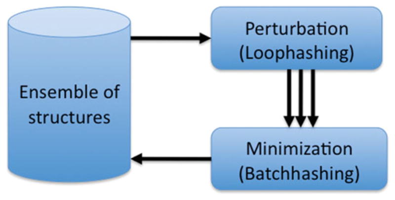
Overall schematic of sampling. Parallel loophash sampling (PLS) is based on repeated cycles of two operations: a) a one-to-many perturbation operation generating many variants and b) a many-to-one minimization in which batches of structures compete for a final winning structure. This approach differs from most classical sampling algorithms which only use one-to-one operations. Our scheme is not only much more efficient but also allows for straightforward parallelization. [Color figure can be viewed in the online issue, which is available at wileyonlinelibrary.com.]

Although this type of conformational space search has been around for many decades, the devil is in the details. Here, we present a number of developments that considerably speed up the process, thereby significantly increasing the number of samples examined. We first discuss the Loophash and Batchrelax algorithms in detail. We then show how the entire sampling algorithm is structured from these basic components and how it can be parallelized to efficiently use a very large number of processing cores.

Loophash

Loophash is an extremely fast algorithm for rebuilding segments of a protein structure without changing the geometry of the remainder of the structure in internal coordinates. The word “loop” is used loosely in this article and can denote any short segment of the protein chain independent of its secondary structure. The algorithm relies on a precomputed library of protein segments typically, but not necessarily, derived from the protein database (PDB). A database of protein segments (fragments) is generated and then indexed by the rigid body transform (RBT) between the coordinate frames of the first and last residue of each segment in the database.

To create the database, the entire PDB is broken down into fragments, and the RBT is calculated for each fragment. The RBT is a six-dimensional quantity composed of a translational vector (D_x, D_y, D_z) and three Euler angles (α, β, γ) that describe the coordinate transformation from the first to the last amino acid of each fragment. We discretize each component (the translational bin size is ~2 Å wide, the angular bin size is ~25°) and then create a unique index for this RBT bin. The index is then entered into a hash table for rapid retrieval. To keep the database in memory efficiently, we store the three backbone angles (Φ, Ψ,Ω) as 16-bit integers (giving ~0.005° resolution). Each loop entry is simply a pointer into the backbone database so that overlapping loops with backbone angles in common do not have to be stored independently. Using this system, the entire PDB can be stored in a total of 50 megabytes plus 30 megabytes for each length of loop, and hence can be kept in computer memory for fast access during the simulation.

Using this database, it is extremely efficient to obtain all variants for any given segment of a protein that, if substituted, would cause minimal disruption to the rest of the protein. First, a segment is selected and the RBT calculated and discretized (Fig. 2A). The resulting hash key is used to query the hash table of the database and retrieve the bin containing all segments of the specified length and matching RBT (Fig. 2B). The segments are filtered to assure that only residues with compatible backbone geometry are inserted; this is particularly important for glycine, proline, and β-branched residues. For example, a segment containing a residue with a Φ angle outside of −103° to −33° cannot be inserted if that position coincides with a proline residue. Next, the torsion angles of the segment in question are replaced by one of the torsion angle sets retrieved from the database. These torsion angle changes move the downstream portion of the protein by a substantial amount because the RBT was discretized and will not match perfectly (Fig. 2C). To alleviate this so-called lever effect, two short gradient-descent minimizations (using the Davidson–Fletcher–Powell method) are performed with harmonic constraints applied to the original Cα coordinates of the structure. During the first minimization, only the torsion angles of the inserted segment are allowed to move. In the second minimization, all backbone torsion angles are allowed to move (Fig. 2D). These minimization steps are extremely fast because they are driven only by the constraints and simple steric repulsion forces and are performed with a centroid representation of the structure. When repeated for all matching segments found in the hash-bin, the result is a set of variant structures, which differ from the starting structure only in a local segment.

Figure 2.

Creating structure variants with Loophash. A) We select an arbitrary segment and calculate the RBT between coordinate frames of the first and last amino acid. The resulting RBT is discretized. B) We query the hash table of the precalculated database with the calculated RBT and use it to retrieve the bin containing all segments of the specified length and which match the RBT. This operation is extremely fast (less than 0.1% of central processing unit (CPU) time is spent retrieving segments). C) For each retrieved segment, we apply the torsion angles to the current structure (one by one.) Because the RBT of the new segment matches that of the old, the lever effect is minimized. However, some lever arm motion remains, due to the discretization (binning) of the RBT in step A. D) To remove the remaining lever arm distortion, we perform two short gradient-descent minimizations (using the Davidson– Fletcher–Powell (DFP) method) with harmonic constraints applied between the new and the original Ca coordinates of the structure. During the first minimization, only the torsion angles of the inserted segment are allowed to move, whereas the second minimization allows all backbone torsion angles to move.

Depending on the nature of the input library, Loophashing satisfies the third and fourth principles outlined in the Introduction Section. The library can be made either from the whole PDB or from an existing pool of structures specific to the case being simulated. The latter is often useful for homology modeling problems, where a number of candidate threading models are available.

We benchmarked the speed of several Rosetta Loopbuilding methods. On a modern CPU, the time required to build a closed 12-residue loop on a 202-residue protein using Loophash is only 2 s (compared with 23 s for the Rosetta fragment-based loop builder^[6] and 260 s with Kinematic Loopclosure^[22]). Of course, it should be noted that, unlike the other two algorithms, Loophash takes the liberty of changing the regions outside the loop very slightly and is thus not strictly a loop-building protocol. Typical deviation from the starting structure outside of the remodeled loop is 0.4–1.5 Å. However, in the context of many protocols, especially sampling, such small deviations are permissible, if not, in fact, desired.

Batchrelax

The loop building operations described above take place in a simplified (“centroid”) representation of the protein to increase speed. The next step is to transform these low-resolution models into a physically realistic all-atom representation. This step is referred to as “relax”, as the structure is allowed to relax into a new physical representation to relieve clashes and pack the side chains in a low-energy arrangement.

Because the shape of the local energy landscape is dominated by short range forces, the local energy gradient gives little or no indication of the direction of the global minimum or even deep nearby local minima beyond the immediate local minimum. Thus, gradient-based minimization will not help to move structures toward the global minimum. Instead, it will only return the energy and location of the nearest local minimum and thus acts merely as an expensive way to score the local fitness. It follows that one should only minimize as far as is necessary to distinguish structures according to their relative fitness, because any minimization beyond this only wastes compute cycles. Thus, the Fastrelax and Batchrelax have been designed to return a representative full-atom energy as fast as possible, allowing the overall algorithm to proceed.

The Fastrelax algorithm comprises interlaced cycles of full combinatorial repacking of the side-chains of the protein (repack) and gradient-based minimization of the backbone and side-chain degrees of freedom (minimize). These cycles are repeated four times while the strength of the repulsive weight is varied; starting at a low weight of 2% of the final repulsive weight, the weight is ramped over four cycles of repack/minimize to its final value, comprising a full Fastrelax round. Typically 5–15 rounds of repulsive weight annealing are applied to a given structure, and the lowest energy structure encountered (only full repulsive weight structures are eligible) is finally kept as the result. This algorithm has been shown to be up to seven times more efficient than the original relax algorithm in ROSETTA.^[23,24]

The Batchrelax algorithm is a specialized version of Fastrelax for situations where many structures are to be relaxed and a single, best-energy structure is to be selected to go into another round of any given iterative algorithm. In this situation, it is considerably more efficient to let multiple structures progress through the steps of Fastrelax in parallel. At each step, the structures are sorted by energy and aggressively discarded (up to 75% at each step). This reduces the number of computationally expensive repack and minimization steps required and results in a single lowest energy structure.

This process takes advantage of the relatively good correlation in energy between the start and final energies of each structure (See Supporting Information Fig. S2). Batchrelax is 4– 10 times more efficient at generating low-energy all-atom structures than the Fastrelax procedure (depending on the stringency of discarding step) and up to 70 times more efficient than the original Classicrelax procedure from Kuhlman et al.^[23]

Parallel loophash sampling

Modern computer architectures are moving toward high parallelism and thus parallelizability is of key importance in a new algorithm. Here, we present a new scheme for protein structure sampling on a massively parallel computer such as Bluegene. It improves on our previously published schemes such as ILR^[6] and the “Archive” system that has been successfully used on the recently published RASREC system.^[25] These systems for parallelization are limited to from a few hundred CPUs up to 2000 CPUs. Parallel loophash sampling (PLS), on the other hand, is designed to successfully parallelize over up to 128,000 CPUs or more.

As with RASREC, ILR, and other published algorithms,^[2] our new algorithm refines an ensemble of structures (typically a pool of 50–500 structures) concurrently, rather than simulating many independent sampling trajectories. This allows it to ensure that the conformational space search does not over-converge and provides an opportunity for different search paths to share their finds by exchanging fragments between structures in the ensemble. However, PLS differs from other algorithms in a number of critical ways. First, we abandoned the concept of distinct generations of structures and opted for a continuous-flow architecture. This prevents worker nodes from idling while waiting for a generation to complete. Furthermore, discrete populations often require an interlaced processing step^[6,25] (e.g., clustering), which is frequently not well parallelizable and holds up all the worker processes. This was a major factor in preventing ILR from scaling to larger computer clusters and larger structure pools.

Instead, PLS has a three-tiered hierarchical system instead of the simpler two-tiered system of ILR or the RASREC system. This distributes the work of coordinating different work units over a number of nodes and thus removes the previous communication bottleneck.

As shown in Figure 3A, PLS comprises a single Emperor node, a variable number of Master nodes (typically in the hundreds) and a very large number of worker nodes. This reduces the overall communication requirements and allows PLS to parallelize up to 128,000 CPUs with very good efficiency. The scaling of PLS is shown in detail in Figure 4C.

Figure 3.

Parallelization of Loophash sampling (PLS). A) Overall architecture of PLS. One Emperor node typically drives 100–200 Masters, which in turn drive hundreds of Slave nodes each. All the perturbation and minimization work happens on the Slave nodes, whereas the workflow management occurs on the Master nodes. Slaves do not have to be necessarily bound strictly to one Master but can change their assignment, easing load balancing. However, any finished work is always returned to the Master that sent it. B) Details of the information flow in PLS. The Emperor in red manages the overall ensemble to be refined. It sends new structures to the Masters on request. Each Master operates on one current structure, which is used to generate variants using the Loophash algorithm. Instead of locally performing this, the work is packaged in work units and sent out to available Slaves for execution. Once done, the Slaves send back the variants to their respective Masters, which then repackage the (centroid) variants to be Batchrelaxed. Finally, the winners of each Batchrelax are returned to the Masters and subjected to a metropolis criterion. If accepted, the returned structure replaces the current structure on the Master. In addition, the accepted structure is reported to the Emperor, which will integrate the new structure into the overall ensemble according to a diversity rule (for details see text).

Figure 4.

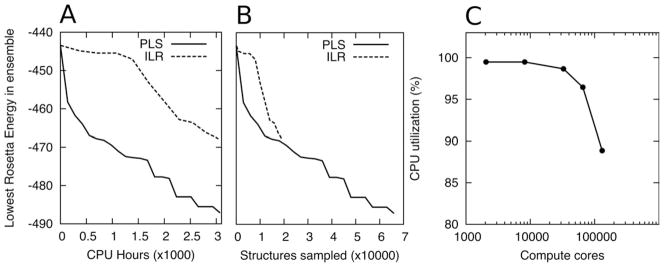
Performance test of PLS. A) Comparison of PLS (solid line) with ILR (dashed line). The lowest energy of the sampling ensemble is plotted against the total number of CPU hours spent (Protein is T297, 211 Residues). PLS is able to find lower energy structure in considerably less computational time. B) PLS and ILR find similar energies for a given amount of samples. The ability of PLS to explore conformational space more efficiently thus stems chiefly from the fact that it is able to explore a much larger number of structures per unit CPU time due to the more efficient component algorithms presented. For T297 (a 211 residue protein), PLS explores about 35 structures per CPU hour whereas ILR only explores around 7. C) Computational efficiency when scaling over very large numbers of processors. Due to the hierarchical distribution of work, PLS parallelizes extremely well. We keep the ratio of Masters to Slave nodes constant when scaling, ensuring continuing supply of work nodes for the Slaves nodes. Ultimately (at ~128000 CPUs), the Emperor node begins to saturate with network traffic, and the efficiency decreases.

PLS is implemented using the message passing interface (MPI) standard for message passing and can be run on any commodity cluster with MPI or on large high performance clusters (HPC) such as Bluegene. Because of the hierarchical nature of the protocol, this protocol is usually not limited by network traffic but by CPU limits. Although the system described is general with respect to the protocol, we will describe it below as used to implement a sampling strategy (PLS), comprising both the Loophash and the Batchrelax algorithms.

A further advantage of PLS over ILR is that it is possible to, in addition to the PDB, hash the input structures and the running ensemble and add them to the fragment libraries. This provides a mechanism to exchange structural features between members of the ensemble. In the case of homology modeling, this can be a powerful feature to bias the sampling toward lower energies and more native-like structures. The roles of the nodes at each level are described in the following paragraphs.

Emperor node

The ensemble of structures (global structure library) is kept and maintained on the Emperor node. The Master nodes coordinate short individual sampling trajectories and report to the Emperor any structure that successfully passed the Metropolis criterion (see below for details). These structures are added to the global structure library using a diversity rule. This rule, also used by RASREC and ILR, determines the structurally closest member in the current pool. If the CαRMSD to that closest structure is below a certain CαRMSD cutoff, the two structures compete for their spot in the pool, with the lower energy structure winning out. If the closest member deviates by more than the cutoff CαRMSD from the new candidate structure, then the new structure is simply added to the pool. If the size of the pool has now exceeded the maximum size, the worst energy structure of the entire pool is discarded.

The Emperor can also be used to create a Loophash library from the structures in the pool rather than from the entire PDB. This library can then be distributed to the Slave nodes and used to create new variant structures. This mechanism allows recombination within the pool of structures.

Master nodes

Each Master holds a “current structure” that is being refined using alternating rounds of Loophash and Batchrelax. It also maintains a queue of work units. Whenever the queue becomes empty, the Master creates more Loophash work units that are sent out to the Slaves. Each work unit contains a copy of the current pose and instructions to execute Loophash on a small section of that pose (typically, a stretch of 15–25 residues). The work units are sent to the Slaves, which generate new centroid poses with new loop segments inserted. The results are returned to the Master and are then divided up into batches and sent out again as Batchrelax work units. Once again, the processing occurs only on the Slave nodes. The resulting, relaxed, all-atom structures are then returned to the Master and compared to the current pose using the Metropolis criterion ^[1] at a suitable temperature (typically around 2.5).

Successfully accepted structures are also passed on to the Emperor node which then integrates that structure into the overall pool as described above. Once a sufficient number of structures have been returned without an acceptance event, that is, when the trajectory is stuck, the Master will return the current structure to the Emperor and request a new structure to work on. This ensures the protocol does not get stuck in dead ends, wasting compute cycles.

Slave nodes

Each Slave node is permanently assigned a Master from which it periodically receives work units. Each work unit contains input protein structures and instructions on what procedures are to be executed on them. Both are serialized and sent over MPI from the Master to the Slave. Structures are sent and received as “SilentStructures” rather than PDBs due to their favorably compact size. The “Silent” format is a text file format that stores internal degrees of freedom of a structure rather than coordinates and is used internally by Rosetta. When a work unit (WU) is received on the Slave, it is unpacked and the commands are executed on each structure. The output structures are placed in the work unit data structure (replacing the input structures) and the work unit is returned to the Master. The Slave then advertises itself as available for more work.

Work units may create structures in a number of ways: one-to-one, one-to-many, many-to-one, or many-to-many. Loophash is a one-to-many protocol (one input structure yields many output structures), whereas Batchrelax is a many-to-one style protocol (many input structures result in one final relaxed winner structure).

Results

Parallel loophash sampling (PLS) aims to provide more efficient and deeper exploration of the energy landscape of proteins than previous methods using the new algorithms for perturbations and minimization described above. To evaluate the algorithm, we subjected it to a number of tests and comparisons with previous algorithms.

Results of benchmark comparison

We compared PLS with our older ILR procedure^[6] head-to-head on a 211 residue sampling problem (T0297 from CASP7). The starting population comprises 200 starting structures generated by the Rosetta homology modeling pipeline.^{[ 26]} Each algorithm was allowed to run for ~3000 CPU hours. Figure 4A plots the lowest energy in the ensemble against consumed computer time and shows that PLS descends to low energies considerably faster than ILR (around three to five times depending on the stage of the algorithm). Figure 4B shows the same data plotted versus the number of structures sampled. The difference between the graphs is considerably smaller, suggesting that the improved performance stems mainly from the ability of PLS to sample more structures. The fragment insertions performed by PLS are only slightly more effective than those generated by the loop-building algorithm used in ILR, but due to the increased computational efficiency of the loop building and relax phases, three times more structures are generated in the same amount of time. As discussed in the Introduction Section, when conformational spaces are extremely rugged and individual minima lack any sense of direction toward a global minimum, only increased sampling and heuristic recombination of previously found low minima, such as implemented in PLS, are able to improve the search.

Result of Loophash on small proteins (50–150aa)

To investigate the effectiveness of the new method in finding low energy structures, we performed a benchmark on 31 proteins. For each protein, we generated a starting set of 200–300 structures using the standard ROSETTA ab initio prediction protocol,^[27] consisting of ROSETTA ab initio prediction run followed by a simple Fastrelax run. To increase diversity and coverage of the structures, we seeded in simulations with varying degrees of native bias.^[27] Each set of 200–300 structures was loaded into the PLS as the starting population and refined on 4192 CPU cores for a total duration of 12 h on a Bluegene Supercomputer (Intrepid). The fragment library was derived from the entire PDB.

Figure 5 shows the lowest energy of the refined structures at various CαRMSDs for four of the 31 examined proteins. The results show that for both near-native (low-CαRMSD) and far from native (high-CαRMSD) the sampling algorithm is capable of finding states with much lower energy than previously possible. In the study above,^[27] energy landscape exploration was performed using a large number of independent trajectories of Fastrelax from a large number of pregenerated centroid structures. This process is considerably less efficient than the algorithm presented in this article. For example, the generation of the data displayed in dashed line in Figure 5 alone required a roughly equal amount of CPU time compared to the sampling runs performed here (results in red), yet the latter is able to penetrate considerably deeper into the energy landscape.

Figure 5.

Energy landscapes and alternative minima revealed by Loophash. The solid black line indicates the lowest energy by CαRMSD for the final refined set after 50,000 CPU hours of sampling. In all cases, previously unseen minima are exposed through the sampling process (indicated by circles). Many of the minima are comparable in energy to low CαRMSD structures that are close to the native structure. The full set of results is presented in the Supporting Information. The dashed line indicates the lowest energy by CαRMSD obtained using the landscape exploration method used in our previous study^[27] using a roughly equal amount of total computational power.

The most striking feature of these new energy landscapes is that in many cases where previously a funnel-like structure toward the native state was seen it now appears flat or contains minima which are comparable or lower in energy than the native basin but are structurally dissimilar. These competitive non-native minima are observed for 14 of the 31 proteins examined.

Result of Loophash on larger proteins (>200aa)

Figure 6 shows the results of Loophash applied to two homology modeling targets from CASP7, T0286, and T0297, with 202 and 211 amino acids, respectively. For comparison, we also show results obtained previously using ILR, an older technique used in CASP7.^[6] This algorithm also uses repeat cycles of loop rebuilding and all-atom Relax, but comprises older and less efficient algorithms for both.

Figure 6.

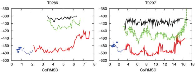
Alternative minima revealed by Loophash for two large proteins from CASP7 (T0286, 202 residues, T0297, 211 residues). Each graph shows the lowest energy at various RMSD values for a given set of structures. Absence of a line in a certain RMSD range indicates that there were no structures sampled at that RMSD. Black solid line → starting population; Dashed green line → previous best sampling result (using ILR); Red solid line → sampling using Loophash (PLS); Blue points → relaxed native structures; Blue dashed line → relaxed native structures refined with Loophash. [Color figure can be viewed in the online issue, which is available at wileyonlinelibrary.com.]

Both runs were initiated with identical sets of ~200 diverse starting structures generated by the standard ROSETTA template modeling pipeline.^[26] The same 200 structures were also hashed into the input fragment library allowing exchange of features between different structures.

In both examples, PLS reaches far lower energies than ILR. In the case of T0286, PLS also explores structures much closer to the native structure than ILR (lower CαRMSD values). In the case of T0297, no improvement in CαRMSD is seen, despite quite dramatic improvements in energy. In both examples, the lowest energies obtained after Loophash are lower than or equal to those of the native structure with no apparent funnel. This failure of the energy function precludes any further progress toward the native structure for these proteins. However, these newly exposed minima will be invaluable in guiding improvements to the ROSETTA energy function. Before the application of PLS, it was not possible to improve the energy function, as the available data suggested the presence of a sufficient energy gap, and thus the inability to find the native structure was blamed on insufficient sampling. With the sampling problem significantly alleviated, we can now conclude from these experiments that the energy function is not currently suitable for consistent high-accuracy structure prediction.

This conclusion is further corroborated by applying the Loophash algorithm to the native structure itself (blue dashed line in Fig. 6). In both examples T0286 and T0297, the Loophash algorithm is able to improve the energies of the native structure by moving it away from the native coordinates. This shows that the ROSETTA energy function does not ascribe the native structure to a deep minimum, as it should.

Conclusions

We have described a superior sampling algorithm which incorporates novel approaches to variant structure generation, all-atom energy minimization, and parallelization strategies. Tests of the algorithm’s ability to explore the energy landscape more efficiently show that completely unknown energy minima can be found using this technique.

For the first time in several years, it appears in many cases that successful protein structure prediction is no longer only limited by ability to sample^[14] but by accuracy of the energy function. We are currently using this data to improve the Rosetta Energy function by adding new terms to address physical effects that were previously unaccounted for.

Due to the current insufficiencies of pure ab initio prediction, the incorporation of weak or sparse experimental data has proven to be an extremely constructive path. For example, the use of chemical shift data,^[28] residual dipolar coupling (RDC) data,^[29] ILV NOE data,^[30] or electron density from electron diffraction studies^[31] has enabled the Rosetta to generate accurate models for many proteins. These data provide additional constraints to the search for the native state, not only guiding and concentrating the search into smaller areas of conformational space but also offsetting some of the inaccuracies in the Rosetta all-atom force-field. The approach described here should be particularly powerful in conjunction with such data.

APPENDIX

Rosetta (including the PLS protocol presented here) is open-source for academic and not-for-profit uses and is freely available from http://www.rosettacommons.org/software/ and comes with extensive documentation (available at http://www.rosettacommons.org/manual_guide)

Example command lines for running PLS:

Creating Loophash database from a collection of PDB files

To create a database from PDB files use this command:

loophash_createdb.mpi.linuxgccrelease -lh:db_
path ./ -database <rosetta_database_path> -
in:file:s *.pdb -lh:loopsizes 10 15 20

Running PLS on a commodity computer cluster with MPI

To start a loophash job using MPI use

mpirun loophash_mpi.mpi.linuxgccrelease <flags>

Typical flags

-database <rosetta_database_path>     ## location of rosetta database
-lh:jobname myjob                  ## jobname prefix
-in:file:silent <inputfile>             ## The starting population
-lh:db_path <loophash_database_path>  ## where the loop database is (previous step)
-lh:library_expiry_time 1200          ## time after which unsuccessful Master thread aborts
-lh:loopsizes 10 15 20                ## The different lengths of loops to be used
-lh:max_emperor_lib_size 40          ## How big a pool of structures should be maintained
-lh:max_lib_size  1                 ## How many threads per Master (usually just 1)
-lh:mpi_batch_relax_chunks  16       ## How big should the Batchrelax batches be
-lh:mpi_loaphash_split_size 3         ## How many consecutive residues to be handles together
-lh:mpi_metropolis_temp 2.5          ## Monte Carlo temperature
-lh:max_loophash_per_structure 4      ## How many times to try loophashing any unique structure
-lh:mpi_save_state_interval 3600       ## Save state of simulation once an hour
-lh:rms_limit 1.5                    ## Diversity rule for Emperor (1.5 A RMS)
-wum:;n_masters 200                ## How many Master nodes
-native native.pdb                   ## If present, use this PDB as a reference to calculate RMS
-relax:script script_file               ## Batchrelax script (detailed steps for Batchrelax)

Typical Batchrelax script

ramp_repack_min 0.02  0.01
batch_shave 0.25
ramp_repack_min 0.250 0.01
batch_shave 0.25
ramp_repack_min 0.550 0.01
batch_shave 0.25
ramp_repack_min 1    0.00001
accept_to_best
ramp_repack_min 0.02  0.01
ramp_repack_min 0.250 0.01
batch_shave 0.25
ramp_repack_min 0.550 0.01
ramp_repack_min 1    0.00001
accept_to_best
ramp_repack_min 0.02  0.01
ramp_repack_min 0.250 0.01
batch_shave 0.25
ramp_repack_min 0.550 0.01
ramp_repack_min 1    0.00001
accept_to_best
ramp_repack_min 0.02  0.01
ramp_repack_min 0.250 0.01
batch_shave 0.25
ramp_repack_min 0.550 0.01
ramp_repack_min 1    0.00001
accept_to_best

References

- 1.Li Z, Scheraga HA. Proc Natl Acad Sci USA. 1987;84:6611. doi: 10.1073/pnas.84.19.6611. [DOI] [PMC free article] [PubMed] [Google Scholar]
- 2.Lee J, Scheraga HA, Rackovsky S. J Comp Chem. 1997;18:1222. [Google Scholar]
- 3.Byrne D, Li J, Platt E, Robson B, Weiner P. J Comput Aided Mol Des. 1994;8:67. doi: 10.1007/BF00124350. [DOI] [PubMed] [Google Scholar]
- 4.Sugita Y, Okamoto Y. Chem Phys Lett. 1999;314:141. [Google Scholar]
- 5.Wenzel W, Hamacher K. Phys Rev Lett. 1999;82:3003. [Google Scholar]
- 6.Qian B, Raman S, Das R, Bradley P, McCoy AJ, Read RJ, Baker D. Nature. 2007;450:259. doi: 10.1038/nature06249. [DOI] [PMC free article] [PubMed] [Google Scholar]
- 7.Berne BJ, Straub JE. Curr Opin Struct Biol. 1997;7:181. doi: 10.1016/s0959-440x(97)80023-1. [DOI] [PubMed] [Google Scholar]
- 8.Christen M, Gunsteren WFv. J Comput Chem. 2008;29:157. doi: 10.1002/jcc.20725. [DOI] [PubMed] [Google Scholar]
- 9.Carr JM, Wales DJ. Phys Chem Chem Phys. 2009;11:3341. doi: 10.1039/b820649j. [DOI] [PubMed] [Google Scholar]
- 10.Lidar DA, Thirumalai D, Elber R, Gerber RB. Phys Rev E. 1999;59:2231. [Google Scholar]
- 11.Wolpert DH, Macready WG. IEEE Trans Evol Comput. 1997;1:67. [Google Scholar]
- 12.Glover F. ORSA J Comput. 1989;1:190. [Google Scholar]
- 13.Simons KT, Bonneau R, Ruczinski I, Baker D. Proteins. 1999;(Suppl 3):171. doi: 10.1002/(sici)1097-0134(1999)37:3+<171::aid-prot21>3.3.co;2-q. [DOI] [PubMed] [Google Scholar]
- 14.Bradley P, Misura KMS, Baker D. Science. 2005;309:1868. doi: 10.1126/science.1113801. [DOI] [PubMed] [Google Scholar]
- 15.Pedersen JT, Moult J. Curr Opin Struct Biol. 1996;6:227. doi: 10.1016/s0959-440x(96)80079-0. [DOI] [PubMed] [Google Scholar]
- 16.Hess B, Kutzner C, van der Spoel D, Lindahl E. J Chem Theor Comp. 2008;4:435. doi: 10.1021/ct700301q. [DOI] [PubMed] [Google Scholar]
- 17.Fitcha BG, Germaina RS, Mendellb M, Piterac J, Pitmana M, Rayshubskiya A, Shama Y, Suitsa F, Swopec W, Warda TJC, Zhestkova Y, Zhoua R. J Parallel Distrib Comput. 2003;63:759. [Google Scholar]
- 18.Phillips JC, Braun R, Wang W, Gumbart J, Tajkhorshid E, Villa E, Chipot C, Skeel RD, Kale L, Schulten K. J Comput Chem. 2005;26:1781. doi: 10.1002/jcc.20289. [DOI] [PMC free article] [PubMed] [Google Scholar]
- 19.Shaw DE, Deneroff MM, Dror RO, Kuskin JS, Larson RH, Salmon JK, Young C, Batson B, Bowers KJ, Chao JC, Eastwood MP, Gagliardo J, Grossman JP, Ho CR, Ierardi DJ, Kolossváry I, Klepeis JL, Layman T, McLeavey C, Moraes MA, Mueller R, Priest EC, Shan Y, Spengler J, Theobald M, Towles B, Wang SC. In Proceedings of the ACM/IEEE Conference on Supercomputing (SC09) ACM Press; New York: 2009. [Google Scholar]
- 20.Snow CD, Nguyen H, Pande VS, Gruebele M. Nature. 2002;420:102. doi: 10.1038/nature01160. [DOI] [PubMed] [Google Scholar]
- 21.Levitt M. J Mol Biol. 1983;170:723. doi: 10.1016/s0022-2836(83)80129-6. [DOI] [PubMed] [Google Scholar]
- 22.Mandell D, Coustias EA, Kortemme T. Nat Methods. 2009;6:551. doi: 10.1038/nmeth0809-551. [DOI] [PMC free article] [PubMed] [Google Scholar]
- 23.Kuhlman B, Dantas G, Ireton GC, Varani G, Stoddard BL, Baker D. Science. 2003;302:1364. doi: 10.1126/science.1089427. [DOI] [PubMed] [Google Scholar]
- 24.Khatib F, Cooper S, Tyka M, Xu K, Makedon I, Popović Z, Baker D. Proc Natl Acad Sci USA. 2011;108:18949. doi: 10.1073/pnas.1115898108. [DOI] [PMC free article] [PubMed] [Google Scholar]
- 25.Lange OF, Rossi P, Sgourakis NG, Song Y, Lee H, Aramini JM, Ertekin A, Xiao R, Acton TB, Montelione GT, Baker D. Proc Natl Acad Sci USA. 2012;109:10873. doi: 10.1073/pnas.1203013109. [DOI] [PMC free article] [PubMed] [Google Scholar]
- 26.Raman S, Vernon R, Thompson J, Tyka M, Sadreyev R, Pei J, Kim D, Kellogg E, DiMaio F, Lange O, Kinch L, Sheffler W, Kim BH, Das R, Grishin NV, Baker D. Proteins. 2009;77:89–99. doi: 10.1002/prot.22540. [DOI] [PMC free article] [PubMed] [Google Scholar]
- 27.Tyka M, Keedy DA, André I, DiMaio F, Song Y, Richardson DC, Richardson JS, Baker D. J Mol Biol. 2011;405:607. doi: 10.1016/j.jmb.2010.11.008. [DOI] [PMC free article] [PubMed] [Google Scholar]
- 28.Shen Y, Lange OF, Delaglio F, Rossi P, Aramini JM, Liu G, Eletsky A, Wu Y, Singarapu KK, Lemak A, Ignatchenko A, Arrowsmith CH, Szyperski T, Montelione GT, Baker D, Bax A. Proc Natl Acad Sci USA. 2008;105:4685. doi: 10.1073/pnas.0800256105. [DOI] [PMC free article] [PubMed] [Google Scholar]
- 29.Raman S, Lange OL, Ross P, Tyka M, Wang X, Aramin J, Liu G, Ramelot RA, Eletsky A, Szyperski T, Kennedy MA, Prestegard J, Montelione GT, Baker D. Science. 2009;19:1014. doi: 10.1126/science.1183649. [DOI] [PMC free article] [PubMed] [Google Scholar]
- 30.Sgourakis NG, Lange OF, DiMaio F, Andre I, Fitzkee NC, Rossi P, Montelione GT, Bax A, Baker D. J Am Chem Soc. 2011;133:6288. doi: 10.1021/ja111318m. [DOI] [PMC free article] [PubMed] [Google Scholar]
- 31.DiMaio F, Tyka MD, Baker ML, Chiu W, Baker D. J Mol Biol. 2009;392:181. doi: 10.1016/j.jmb.2009.07.008. [DOI] [PMC free article] [PubMed] [Google Scholar]
Associated Data
This section collects any data citations, data availability statements, or supplementary materials included in this article.