Why Do More Divergent Sequences Produce Smaller Nonsynonymous/Synonymous Rate Ratios in Pairwise Sequence Comparisons?

Abstract

Several studies have reported a negative correlation between estimates of the nonsynonymous to synonymous rate ratio (ω = d_N/d_S) and the sequence distance d in pairwise comparisons of the same gene from different species. That is, more divergent sequences produce smaller estimates of ω. Explanations for this negative correlation have included segregating nonsynonymous polymorphisms in closely related species and nonlinear dynamics of the ratio of two random variables. Here we study the statistical properties of the maximum-likelihood estimates of ω and d in pairwise alignments and explore the possibility that the negative correlation can be entirely explained by those properties. We show that the ω estimate is positively biased for small d and that the bias decreases with the increase of d. We also show that the estimates of ω and d are negatively correlated when ω < 1 and positively correlated when ω > 1. However, the bias in estimates of ω and the correlation between estimates of ω and d are not enough to explain the much stronger correlation observed in real data sets. We then explore the behavior of the estimates when the model is misspecified and suggest that the observed correlation may be due to protein-level selection that causes very different amino acids to be favored in different domains of the protein. Widely used models fail to account for such among-site heterogeneity and cause underestimation of the nonsynonymous rate and ω, with the bias being much stronger for distant sequences. We point out that tests of positive selection based on the ω ratio are invariant to the parameterization of the model and thus unaffected by bias in the ω estimates or the correlation between estimates of ω and d.

NATURAL selection acts differently on synonymous and nonsynonymous mutations in protein-coding genes (Kimura 1977). For almost all proteins, the nonsynonymous distance (d_N, measured by the number of nonsynonymous substitutions per nonsynonymous site) is smaller than the corresponding synonymous distance (d_S, measured by the number of synonymous substitutions per synonymous site), because the structure and function of a protein impose constraints on the types of nonsynonymous (amino acid) substitutions that can take place, while synonymous substitutions usually accumulate freely with little or no interference from selection. In contrast, a large nonsynonymous distance (d_N > d_S) is a strong indicator of positive (diversifying) selection acting on the protein (e.g., Messier and Stewart 1997). The nonsynonymous to synonymous rate ratio, ω = d_N/d_S, in a protein-coding gene is thus an important measure of the mode and strength of selection acting on the protein, and it is widely used in detecting positive Darwinian selection [indicated by ω > 1 (Yang and Bielawski 2000)] and also as a descriptive statistic calculated from pairwise sequence alignments.

A number of recent studies have reported a negative correlation between estimates of ω and the evolutionary distance d (the total distance separating the sequences, including nonsynonymous and synonymous changes) in pairwise comparisons of the sequences for the same gene from various organisms (Rocha et al. 2006; Peterson and Masel 2009; Wolf et al. 2009). For example, Rocha et al. (2006) found that pairwise estimates of ω are larger among closely related bacterial genomes. They proposed that deleterious nonsynonymous polymorphisms explain the larger estimates of ω between closely related sequences. As the time of divergence between species increases, nonsynonymous polymorphisms are lost due to purifying selection and the ω ratio decays as a function of time. Similarly, Wolf et al. (2009) reported a negative correlation between estimates of ω and d in comparisons among several mammalian and avian genomes. They argued that this correlation is the result of $\widehat{\omega }$ being the ratio of two random variables (d_N and d_S) and suggested that current statistical tests based on ω (for example, likelihood-ratio tests of positive selection comparing the null hypothesis ω = 1 against the alternative hypothesis ω > 1) are inappropriate in light of the nonlinear behavior of the ratio of random variables.

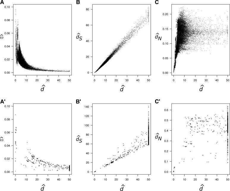
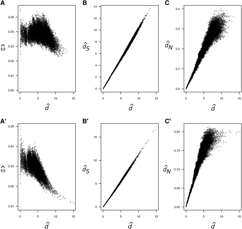
The observed pattern of decay of $\widehat{\omega }$ as a function of $\widehat{d}$ seems to be common (Rocha et al. 2006; Peterson and Masel 2009; Wolf et al. 2009). For example, Figure 1A shows pairwise estimates of ω and d for 12 mitochondrial protein-coding genes from 244 mammal species and Figure 1A′ shows a similar plot for 18 ribosomal protein-coding genes from 49 bacterial species. In both cases, estimates of ω are clearly higher for closely related species, and the estimates decay as a function of the estimated distance. Figure 1, B and B′, shows the estimated synonymous distance d_S vs. estimated d and Figure 1, C and C′, shows the estimated nonsynonymous distance d_N vs. estimated d. Note that estimates of d_S and d are highly correlated in both cases, while estimates of d_N seem saturated for large d.

Figure 1.

Pairwise estimates of ω = d_N/d_S, d, d_S, and d_N for the mitochondrial protein-coding genes of placental mammals (A–C) and ribosomal protein-coding genes of bacteria (A′–C′). (A and A′) Pairwise estimates of ω vs. d. (B and B′) Pairwise estimates of d_S vs. d. (C and C′) Pairwise estimates of d_N vs. d. In A–C the estimates were obtained for all 29,646 comparisons among 244 mammal species, using the program CODEML from the PAML package (Yang 2007), with empirical codon frequencies and assuming no ω variation among sites. The estimates obtained from a joint analysis of all species on the phylogeny are $\widehat{\omega }=0.0376$ and $\widehat{\kappa }=6.33$. The alignment of 244 sequences is 3598 codons long, but only 3411 codons are used after removing alignment gaps. In A′–C′ the estimates were obtained for all 1176 comparisons among 49 bacteria species as for the mammal case. The estimates from the joint analysis are $\widehat{\omega }=0.113$ and $\widehat{\kappa }=1.19$. The alignment is 4324 codons long (1968 codons after removing alignment gaps). The mitochondrial protein-coding genes and the ribosomal protein-coding genes (rplA-rplF and rplI-rplT) were obtained from GenBank.

Pairwise methods ignore the phylogenetic relationships of the species being studied and do not make as efficient use of the information in the sequences as a joint analysis of all sequences on a phylogeny. Nonetheless, pairwise estimates have been widely used, so it is important to understand their limitations. In this article we study the statistical properties of estimates of ω in pairwise sequence alignments, using a combination of techniques, such as mathematical analysis, computer simulation, and real data analysis. We derive the biases in estimates of ω and d, using a fictitious regularized genetic code, and demonstrate similar biases under the universal genetic code, using computer simulation. We then study the impact of heterogeneous selection for amino acids along the protein sequence on estimation of ω and d by computer simulation. Our analysis suggests that the small-sample biases in estimates of ω as well as systematic biases in ω estimates caused by model violation may be important factors to explain the correlation between $\widehat{\omega }$ and $\widehat{d}$ observed in empirical data sets.

Asymptotic Bias and Correlation in Estimates of ω and d

We first consider a simple model of codon evolution that can be treated analytically. Consider a regularized genetic code with 16 amino acids and with every codon fourfold degenerate (Table 1). Substitutions at first and second codon positions are always nonsynonymous and those at the third positions are always synonymous. There are no stop codons. The substitution rate from codon i to j (i ≠ j) is

$$q_{ij}=\{\begin{array}{ll}0,\hfill & \text{for}\hspace{0.5em}\text{more}\hspace{0.5em}\text{than}\hspace{0.5em}\text{one}\hspace{0.5em}\text{change},\hfill \\ \mu ,\hfill & \text{for}\hspace{0.5em}\text{a}\hspace{0.5em}\text{synonymous}\hspace{0.5em}\text{change},\hfill \\ \omega \mu ,\hfill & \text{for}\hspace{0.5em}\text{a}\hspace{0.5em}\text{nonsynonymous}\hspace{0.5em}\text{change}.\hfill \end{array}$$ (1)

The q_ij are the off-diagonal elements of a 64 × 64 rate matrix, Q, with the diagonal elements, q_ii, set such that each row of Q sums to one. Time is measured as the expected number of substitutions per codon site; in other words μ = 1/(6ω + 3) so that $-{\displaystyle \sum q_{ii}/64}=1$. Because every codon position is always either synonymous or nonsynonymous, evolution of codons can be treated as a mixture of two Jukes–Cantor (Jukes and Cantor 1969) models: the first two positions evolve with rate ωμ and the third position with rate μ. Consider a pairwise sequence alignment with n codons and with x_S and x_N observed synonymous and nonsynonymous differences. Let d_S and d_N be the distances at synonymous and nonsynonymous sites, respectively. The total distance between the two sequences is thus d = d_S + 2d_N. It follows that ω = d_N/d_S, and d = (1 + 2ω)d_S. The log-likelihood function is given by the fact that evolution at the first two codon positions and at the third codon position is independent,

$$\begin{array}{c}\ell =x_{\text{S}}\text{log}\left(p_{\text{S}}\right)+\left(n-x_{\text{S}}\right)\text{log}\left(1-p_{\text{S}}\right)\\ +\hspace{0.5em}{x}_{\text{N}}\text{log}\left(p_{\text{N}}\right)+\left(2n-x_{\text{N}}\right)\text{log}\left(1-p_{\text{N}}\right),\end{array}$$ (2)

where

$$p_{\text{S}}=\frac{3}{4}-\frac{3}{4}{e}^{-(4/3)d_{\text{S}}}=\frac{3}{4}-\frac{3}{4}{e}^{-(4d/3\left(1+2\omega \right))},$$ (3)

$$p_{\text{N}}=\frac{3}{4}-\frac{3}{4}{e}^{-(4/3)d_{\text{N}}}=\frac{3}{4}-\frac{3}{4}{e}^{-(4\omega d/3\left(1+2\omega \right))}.$$ (4)

The maximum-likelihood estimates (MLEs) of the distances at synonymous and nonsynonymous sites are, respectively,

$${\widehat{d}}_{\text{S}}=-\frac{3}{4}\text{log}\left(1-\frac{4}{3}{\widehat{p}}_{\mathrm{S}}\right),$$ (5)

$${\widehat{d}}_{\text{N}}=-\frac{3}{4}\text{log}\left(1-\frac{4}{3}{\widehat{p}}_{\text{N}}\right),$$ (6)

where ${\widehat{p}}_{\text{S}}=x_{\text{S}}/n$ and ${\widehat{p}}_{\text{N}}=x_{\text{N}}/\left(2n\right)$ are the observed proportions of synonymous and nonsynonymous differences, respectively. Note that $E\left({\widehat{p}}_{\text{S}}\right)=p_{\text{S}}$ and $E\left({\widehat{p}}_{\text{N}}\right)=p_{\text{N}}$, where E denotes expectation. The MLEs of d and ω are

$$\widehat{d}={\widehat{d}}_{\text{S}}+2{\widehat{d}}_{\text{N}}$$ (7)

(in expected substitutions per codon) and

$$\widehat{\omega }=\frac{{\widehat{d}}_{\text{N}}}{{\widehat{d}}_{\text{S}}}.$$ (8)

There are only two parameters in the model, and we can work either with d and ω or as a different parameterization with p_S and p_N.

Table 1. The fictitious regularized genetic code.

Codon	aa	Codon	aa	Codon	aa	Codon	aa
TTT	A	CTT	E	ATT	I	GTT	M
TTC	A	CTC	E	ATC	I	GTC	M
TTA	A	CTA	E	ATA	I	GTA	M
TTG	A	CTG	E	ATG	I	GTG	M
TCT	B	CCT	F	ACT	J	GCT	N
TCC	B	CCC	F	ACC	J	GCC	N
TCA	B	CCA	F	ACA	J	GCA	N
TCG	B	CCG	F	ACG	J	GCG	N
TAT	C	CAT	G	AAT	K	GAT	O
TAC	C	CAC	G	AAC	K	GAC	O
TAA	C	CAA	G	AAA	K	GAA	O
TAG	C	CAG	G	AAG	K	GAG	O
TGT	D	CGT	H	AGT	L	GGT	P
TGC	D	CGC	H	AGC	L	GGC	P
TGA	D	CGA	H	AGA	L	GGA	P
TGG	D	CGG	H	AGG	L	GGG	P

Note that the regularized genetic code encodes 16 fictitious amino acids, A–P, with no stop codons. Substitutions at the third codon position are always synonymous, while substitutions at the first and second positions are always nonsynonymous.

Both $\widehat{\omega }$ and $\widehat{d}$ are functions of the binomial proportions ${\widehat{p}}_{\text{S}}$ and ${\widehat{p}}_{\text{N}}$ that have variances

$${\sigma }_{{\widehat{p}}_{\text{N}}}^2=\frac{p_{\text{N}}\left(1-p_{\text{N}}\right)}{\left(2n\right)},$$ (9)

$${\sigma }_{{\widehat{p}}_{\text{S}}}^2=\frac{p_{\text{S}}\left(1-p_{\text{S}}\right)}{n},$$ (10)

and $\text{Cov}\left({\widehat{p}}_{\text{S}},{\widehat{p}}_{\text{N}}\right)=0$. Because $\widehat{\omega }$ and $\widehat{d}$ are functions of random variables with known variances, the delta method can be used to calculate the asymptotic expectations

$$E\left(\widehat{d}\right)\approx d+\frac{1}{2}{\sigma }_{{\widehat{p}}_{\text{N}}}^2\frac{{\partial }^2\widehat{d}}{\partial {\widehat{p}}_{\text{N}}^2}+\frac{1}{2}{\sigma }_{{\widehat{p}}_{\text{S}}}^2\frac{{\partial }^2\widehat{d}}{\partial {\widehat{p}}_{\text{S}}^2},$$ (11)

$$E\left(\widehat{\omega }\right)\approx \omega +\frac{1}{2}{\sigma }_{{\widehat{p}}_{\text{N}}}^2\frac{{\partial }^2\widehat{\omega }}{\partial {\widehat{p}}_{\text{N}}^2}+\frac{1}{2}{\sigma }_{{\widehat{p}}_{\text{S}}}^2\frac{{\partial }^2\widehat{\omega }}{\partial {\widehat{p}}_{\text{S}}^2},$$ (12)

and the asymptotic variance/covariance matrix

$$\begin{array}{l}\text{Var}\left(\widehat{d},\widehat{\omega }\right)\\ \hspace{1em}\approx J\cdot \text{Var}\left({\widehat{p}}_{\text{N}},{\widehat{p}}_{\text{S}}\right)\cdot J^T\\ \hspace{1em}=\left(\begin{array}{ll}{\sigma }_{{\widehat{p}}_{\text{N}}}^2{\left(\frac{\partial \widehat{d}}{\partial {\widehat{p}}_{\text{N}}}\right)}^2+{\sigma }_{{\widehat{p}}_{\text{S}}}^2{\left(\frac{\partial \widehat{d}}{\partial {\widehat{p}}_{\text{S}}}\right)}^2\hfill & {\sigma }_{{\widehat{p}}_{\text{N}}}^2\frac{\partial \widehat{d}}{\partial {\widehat{p}}_{\text{N}}}\frac{\partial \widehat{\omega }}{\partial {\widehat{p}}_{\text{N}}}+{\sigma }_{{\widehat{p}}_{\text{S}}}^2\frac{\partial \widehat{d}}{\partial {\widehat{p}}_{\text{S}}}\frac{\partial \widehat{\omega }}{\partial {\widehat{p}}_{\text{S}}}\hfill \\ {\sigma }_{{\widehat{p}}_{\text{N}}}^2\frac{\partial \widehat{b}}{\partial {\widehat{p}}_{\text{N}}}\frac{\partial \widehat{\omega }}{\partial {\widehat{p}}_{\text{N}}}+{\sigma }_{{\widehat{p}}_{\text{S}}}^2\frac{\partial \widehat{b}}{\partial {\widehat{p}}_{\text{S}}}\frac{\partial \widehat{\omega }}{\partial {\widehat{p}}_{\text{S}}}\hfill & {\sigma }_{{\widehat{p}}_{\text{N}}}^2{\left(\frac{\partial \widehat{\omega }}{\partial {\widehat{p}}_{\text{N}}}\right)}^2+{\sigma }_{{\widehat{p}}_{\text{S}}}^2{\left(\frac{\partial \widehat{\omega }}{\partial {\widehat{p}}_{\text{S}}}\right)}^2\hfill \end{array}\right),\end{array}$$ (13)

where $J=\partial \left(\widehat{d},\widehat{\omega }\right)/\partial \left({\widehat{p}}_{\text{N}},{\widehat{p}}_{\text{S}}\right)$ is the Jacobian matrix of the transform (reparameterization). The Jacobian and the second derivatives of $\widehat{\omega }$ and $\widehat{d}$ with respect to ${\widehat{p}}_{\text{N}}$ and ${\widehat{p}}_{\text{S}}$ are given in the Appendix.

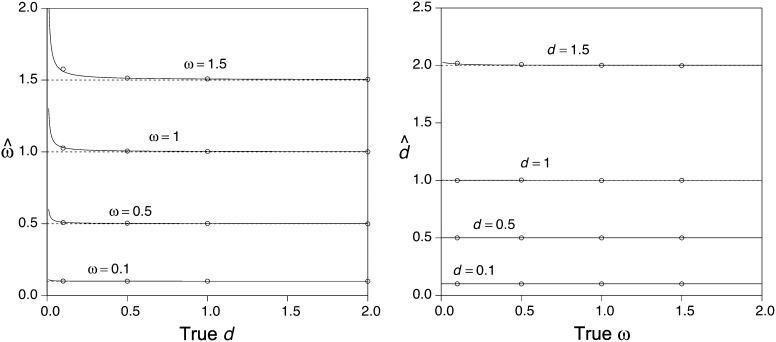
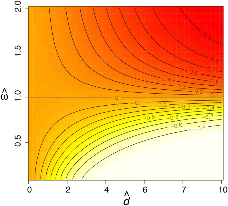
From Equations 11 and 12 the bias of the estimates can be approximated by $E\left(\widehat{d}\right)-d$ and $E\left(\widehat{\omega }\right)-\omega$. Note that when n→∞, $E\left(\widehat{d}\right)\to d$ and $E\left(\widehat{\omega }\right)\to \omega$, as expected according to standard theory. However, when n is small, the bias in the estimators may be substantial. Figure 2 shows the biases of $\widehat{\omega }$ and $\widehat{d}$ for various cases. In particular, there is a positive bias in $\widehat{\omega }$ for small d (Figure 2A). On the other hand, there is very little bias in $\widehat{d}$ (Figure 2B). Simulations confirm that the approximations (Equation 11 and Equation 12) are very good with ≥500 codons in the alignment (Figure 2, A and B). From Equation 13 the asymptotic correlation can be calculated as $\rho \left(\widehat{d},\widehat{\omega }\right)=\text{Cov}\left(\widehat{d},\widehat{\omega }\right)/\sqrt{\text{Var}\left(\widehat{d}\right)\text{Var}\left(\widehat{\omega }\right)}$. Figure 3 shows the asymptotic correlation for various values of ω and d. Calculations indicate that when ω < 1, the correlation is negative (ρ < 0), and when ω > 1, it is positive (ρ > 1).

Figure 2.

Approximate biases of $\widehat{\omega }$ and $\widehat{d}$ for the case of two sequences evolving according to the regularized genetic code. (Left) The expected value of $\widehat{\omega }$ as a function of the true distance d, calculated using Equation 12 when the true ω = 0.1, 0.5, 1, and 1.5. (Right) The expected value of $\widehat{d}$ as a function of the true ω, calculated using Equation 11. In all cases the sequence length is n = 1000 codons. Each open circle is the mean of either $\widehat{\omega }$ or $\widehat{d}$ calculated from 1000 simulated pairwise alignments.

Figure 3.

Correlation between pairwise estimates of ω and d, for the case of two sequences evolving according to the regularized genetic code. The correlation coefficient is calculated from the variance/covariance matrix of Equation 13. The surface represents a topological map where upper (dark) regions show a positive correlation (darkest: ρ = +1.00) and lower (light) regions show a negative correlation (white: ρ = −1.00).

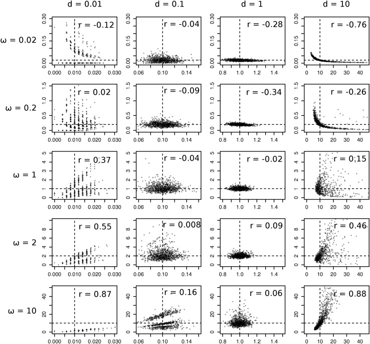
The codon substitution model based on the standard genetic code is not tractable. However, we can study the asymptotic properties of the model by simulation. We simulated pairwise sequence alignments of length n = 500 codons, with equal codon frequencies (1/61) and with κ = 2. We simulated 1000 pairwise alignments for each combination of d = 0.01, 0.1, 1, 10 and ω = 0.02, 0.2, 1, 2, 10 (1000 × 4 × 5 = 20,000 data sets). Estimates of ω and d for each data set were then obtained by maximum likelihood (ML). The simulation shows the same pattern of correlation (Figure 4) as in the case of the regularized code.

Figure 4.

Estimated correlation $\left(r=\widehat{\rho }\right)$ between pairwise estimates of ω and d, for the case of two sequences evolving according to the standard genetic code. The pairwise alignments were simulated with the program EVOLVER, with equal codon frequencies (1/61) and κ = 2. Maximum-likelihood estimates were obtained with CODEML. The dashed lines indicate the true values of ω and d used in the simulations. For some simulated alignments the MLE of d or ω may be ∞. CODEML outputs these values as 50 and 99, respectively. These values are not used in the calculation of r.

To assess whether the bias and correlation of the MLEs of d and ω may be responsible for the strong correlation observed in real data sets, we simulated a 244-species sequence alignment on the mammal phylogeny, using the mitochondrial genetic code. The values of n, ω, and κ and the branch lengths in the simulation were fixed to the MLEs obtained from the joint analysis of the original sequence data. The codon frequencies were fixed to those observed in the real data. Figure 5, A–C, shows the pairwise estimates for this simulation. Although there is a negative correlation between estimates of ω and d, this correlation is much weaker than that observed for the real data (Figure 1A). Furthermore, when the simulated alignment is much longer (when we set n = 10⁶ codons), the correlation almost disappears and the MLE of ω converges to the true value (not shown). The simulation model assumes the same ω for all sites in the gene, which is not realistic for real genes. We also simulated with a different model where ω varies among sites according to a mixture of three site classes [M3 discrete (Yang et al. 2000)]. For the real mitochondrial data under this model, the MLEs are ${\widehat{\omega }}_1=0.00254$, ${\widehat{\omega }}_2=0.0361$, and ${\widehat{\omega }}_3=0.147$, with the estimated frequencies of the site classes being ${\widehat{p}}_1=0.573$, ${\widehat{p}}_2=0.260$, and ${\widehat{p}}_3=0.167$; and $\widehat{\kappa }=7.32$. We then used those parameter values to simulate a 244-species alignment on the mammal phylogeny. Figure 5, A′–C′, shows the pairwise estimates of ω and d (obtained using a model of a single ω for all sites) from this simulated data set. The correlation between $\widehat{\omega }$ and $\widehat{d}$ is stronger, but in general much weaker than for the real data (Figure 1A). Therefore, the asymptotic pattern of correlation and bias seems too weak to explain the pattern observed in real data (Figure 1A).

Figure 5.

Pairwise estimates of ω = d_N/d_S, d, d_S, and d_N for sequence alignments simulated using a model of constant ω among sites (A–C) or using a mixture model of variable ω among sites (A′–C′), using parameter estimates from the 244-species mammalian mitochondrial gene alignment. (A and A′) Pairwise estimates of ω vs. d. (B and B′) Pairwise estimates of d_S vs. d. (C and C′) Pairwise estimates of d_N vs. d.

Variable Selection on Different Domains of the Protein

A major characteristic of protein evolution that has been ignored in the discussion above is among-site heterogeneity. In particular, structural characteristics of real proteins impose constraints on the frequencies of amino acids that vary hugely between protein domains. For example, the core of a protein is composed mainly of hydrophobic amino acids, while the surface of the protein may be composed mainly of hydrophilic amino acids (Baud and Karlin 1999). The active site of an enzyme may tolerate only very few different amino acids that can stabilize a particular substrate and carry out an enzymatic reaction. Halpern and Bruno (1998; see also Tamuri et al. 2012) proposed a codon substitution model based on a population genetics model of site-specific amino acid frequencies. To avoid the use of too many parameters we consider a model of site classes. Suppose there are C site classes. If the protein has n codons, there are n/C codons for each site class. The substitution rate from codon i to j in site class k is given by

$$q_{ij,k}=\{\begin{array}{ll}0,\hfill & \text{for}\hspace{0.5em}\text{more}\hspace{0.5em}\text{than}\hspace{0.5em}\text{one}\hspace{0.5em}\text{change},\hfill \\ \mu ,\hfill & \text{for}\hspace{0.5em}\text{a}\hspace{0.5em}\text{synonymous}\hspace{0.5em}\text{change},\hfill \\ \mu \omega h\left(F_{j,k}-F_{i,k}\right),\hfill & \text{for}\hspace{0.5em}\text{a}\hspace{0.5em}\text{nonsynonymous}\hspace{0.5em}\text{change},\hfill \end{array}$$ (14)

where F_i,k is the fitness of the amino acid encoded by codon i in site class k, and

$$h\left(F_{j,k}-F_{i,k}\right)=\frac{F_{j,k}-F_{i,k}}{1-e^{-\left(F_{j,k}-F_{i,k}\right)}}$$ (15)

is the relative fixation probability of an i to j mutation relative to a neutral mutation (Kimura 1983, p. 45; see also Yang and Nielsen 2008), where h(F_j,k − F_i,k) > 1, = 1, < 1 for F_j,k > F_i,k, F_j,k = F_i,k, and F_j,k < F_i,k, respectively. In other words, selection accelerates or slows down substitutions compared to the rate for a neutral mutation (i.e., when F_j,k = F_i,k). The equilibrium frequency of a given amino acid j in site class k is given by

$${\pi }_{j,k}=\frac{e^{F_{j,k}}}{{\displaystyle \sum e^{F_{i,k}}}}.$$ (16)

If F_j,k = −∞, then π_j,k = 0 and the amino acid is not observed in site class k. The same value of μ is used to scale all rate matrices for the site classes, and μ is set so that time is measured as the expected number of substitutions per site across the gene (i.e., so that $-{\displaystyle {\sum }_{k=1}^C{\displaystyle {\sum }_i{\pi }_{i,k}{q}_{ii,k}/C}}=1$).

The Regularized Genetic Code

We examine whether heterogeneity among sites in amino acid preference may lead to strong correlation between estimates of ω and d under the model of Equation 1 when the data are generated by the process of Equation 14. First we study a simple case under the regularized genetic code (Table 1). There are four classes of sites in the protein, each class corresponding to a group of four amino acids whose codons differ only at the second position. For example, at sites of class I, we observe only amino acids A–D (Table 1); that is, A–D have the same fitness but the other 12 amino acids have fitness −∞. Similarly, class II is composed of amino acids E–H, class III of I–L, and class IV of M–P. The gene is composed of equal proportions of the four site classes (that is, for a gene with 100 codons, 25 belong to class I, 25 to class II, and so on). Note that the substitution rate from codon i to j at a site class can be written as

$$q_{ij}=\{\begin{array}{ll}0,\hfill & \text{for}\hspace{0.5em}\text{more}\hspace{0.5em}\text{than}\hspace{0.5em}\text{one}\hspace{0.5em}\text{change},\hfill \\ 0,\hfill & \text{if}\hspace{0.5em}\text{the}\hspace{0.5em}\text{codons}\hspace{0.5em}\text{differ}\hspace{0.5em}\text{at}\hspace{0.5em}\text{the}\hspace{0.5em}\text{first}\hspace{0.5em}\text{position},\hfill \\ \mu ,\hfill & \text{for}\hspace{0.5em}\text{a}\hspace{0.5em}\text{nonsynonymous}\hspace{0.5em}\text{change}\hspace{0.5em}\text{at}\hspace{0.5em}\text{the}\hspace{0.5em}\text{second}\hspace{0.5em}\text{position},\hfill \\ \mu ,\hfill & \text{for}\hspace{0.5em}\text{a}\hspace{0.5em}\text{synonymous}\hspace{0.5em}\text{change}\hspace{0.5em}\text{at}\hspace{0.5em}\text{the}\hspace{0.5em}\text{third}\hspace{0.5em}\text{position},\hfill \end{array}$$ (17)

where μ = 1/(3ω + 1).

We note the following about this substitution model:

1. the ω ratio at the first codon position is ω₁ = 0 and it is ω₂ = 1 at the second. Therefore, the average ω across the protein is ω = 0.5.

2. Gene-wide, the evolutionary rate is zero at the first codon position and μ at the second and third positions. Therefore, the process can be described by a mixture of two independent Jukes–Cantor processes at the second and third positions.

Let x_N and x_S be the numbers of nonsynonymous and synonymous differences between two sequences of length n codons. The estimates of the nonsynonymous and synonymous distances are

$${\widehat{d}}_{\text{N}}^{\mathrm{*}}=-\frac{3}{4}\text{log}\left(1-\frac{4}{3}{\widehat{p}}_{\text{N}}^{\mathrm{\ast }}\right),$$ (18)

$${\widehat{d}}_{\text{S}}=-\frac{3}{4}\text{log}\left(1-\frac{4}{3}{\widehat{p}}_{\text{S}}\right),$$ (19)

where ${\widehat{p}}_{\text{N}}^{\mathrm{*}}=x_{\text{N}}/n$, instead of ${\widehat{p}}_{\text{N}}=x_{\text{N}}/\left(2n\right)$ as in the model of Equation 1. Then

$${\widehat{d}}^{\mathrm{*}}={\widehat{d}}_{\text{N}}^{\mathrm{*}}+{\widehat{d}}_{\text{S}}$$ (20)

and

$${\widehat{\omega }}^{\mathrm{\ast }}=\frac{{\widehat{d}}_{\text{N}}^{\mathrm{\ast }}}{2{\widehat{d}}_{\text{S}}}.$$ (21)

The factor $\frac{1}{2}$ in the calculation of ${\widehat{\omega }}^{\mathrm{*}}$ is necessary to correct for the zero substitution rate at the first codon position. Let us now assume that ω, d, d_N, and d_S are estimated using the model of Equation 1. We note three points:

1. The synonymous distance d_S is correctly estimated.

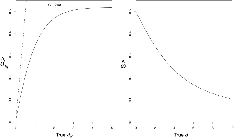
2. The nonsynonymous distance d_N is underestimated and the underestimation is greater for larger sequence divergence (Figure 6A). In fact, the estimate of d_N approaches $-\frac{3}{4}\text{log}\left(1-\frac{1}{2}\right)\approx 0.520$, a constant, as d→∞. The total distance d is also underestimated.

3. As a consequence, ω is underestimated more seriously for longer distances (Figure 6B), and as d→∞, $\widehat{\omega }\to 0$. The correct value of ω is recovered only if the distance is close to zero: d → 0, $\widehat{\omega }\to 0.5$.

Figure 6.

Estimates of d_N (left) and ω = d_N/d_S (right) when the model is misspecified and fails to account for the heterogeneity among sites in amino acid frequencies. The data include infinitely many sites and the regularized genetic code is assumed.

The Standard Genetic Code

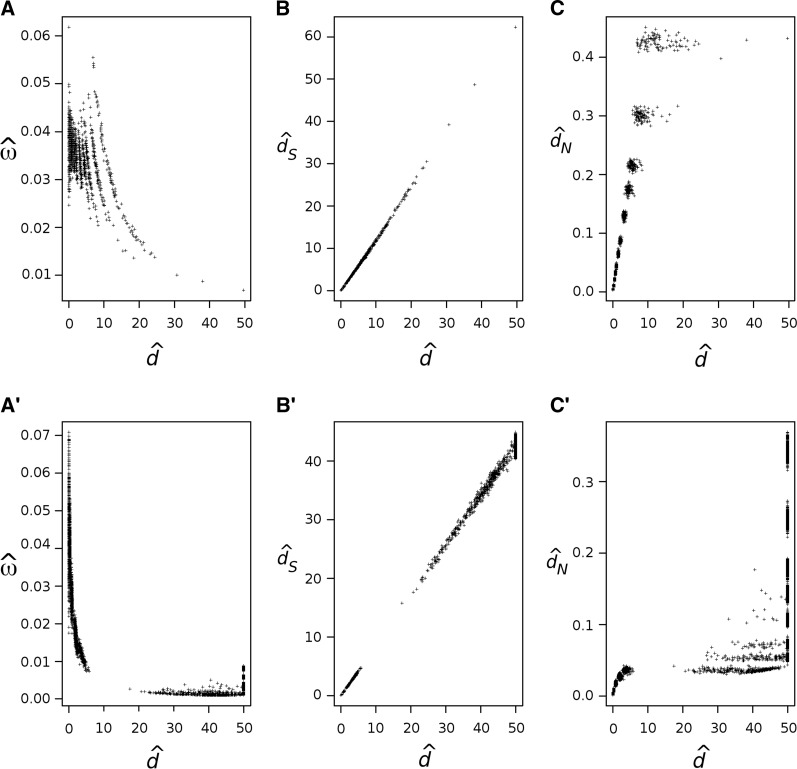
We perform a simulation study, using the standard genetic code. We use two site classes: a class of buried sites in the hydrophobic core of the protein and a class of exposed sites on the protein’s surface. We perform two simulations. The fitnesses for the 20 amino acids for the two site classes are calculated from the literature (Baud and Karlin 1999, Table 2). The substitution model is given by Equation 14, with ω = 0.04 and n = 4000 sites with 2000 sites for each site class. We simulated pairwise sequence alignments for different values of d (= 0.1, 0.25, 0.5, 0.75, 1, 1.5, 2, 3, 4, 5, 7, and 10). The simulation code was written in R. The simulated alignments of two sequences were then analyzed using CODEML to estimate ω and d. The results are shown in Figure 7, A–C. It is clear that ω is underestimated with progressively long distances, causing a negative correlation between estimates of ω and d.

Table 2. Fitnesses and equilibrium frequencies of amino acids in buried and exposed sites in proteins.

	Exposed		Buried
Amino acid	πJ,buried	FJ,buried	πJ,exposed	FJ,exposed
D	0.0214	0	0.0871	0
E	0.0151	−0.348	0.0931	0.067
R	0.0202	−0.061	0.0646	−0.299
K	0.0076	−1.041	0.1021	0.159
H	0.0403	0.633	0.0480	−0.595
L	0.0806	1.326	0.0180	−1.576
M	0.0743	1.244	0.0225	−1.352
I	0.0831	1.356	0.0165	−1.663
V	0.0793	1.301	0.0225	−1.352
F	0.0781	1.294	0.0180	−1.576
W	0.0693	1.174	0.0150	−1.758
Y	0.0567	0.973	0.0225	−1.352
S	0.0416	0.663	0.0661	−0.276
T	0.0441	0.722	0.0586	−0.397
N	0.0264	0.211	0.0811	−0.072
Q	0.0214	0	0.0811	−0.071
C	0.0932	1.471	0.0091	−2.269
G	0.0504	0.856	0.0661	−0.276

Note that amino acid frequencies are taken from Table 1 in Baud and Karlin (1999). The fitnesses are calculated by solving Equation 16 and setting the fitness of asparagine (D) to zero so that F_J,k = log(π_J,k/π_D,k).

Figure 7.

Pairwise estimates of ω = d_N/d_S, d, d_S, and d_N for simulated sequence alignments when the inference model is misspecified under the standard genetic code. (A–C) Estimates for sequences simulated according to the fitnesses of Table 2. (A′–C′) Estimates for sequences simulated with the fitnesses of Table 2 multiplied by 10.

The amino acid frequencies of Table 2 are averaged across different proteins (Baud and Karlin 1999) and may not be as extreme as in individual proteins. To mimic extreme amino acid frequencies in specific proteins, we conducted a second simulation in which the fitnesses for both site classes are multiplied by 10. The results are shown in Figure 7, A′–C′. The underestimation of ω and the negative correlation between estimates of ω and d are more pronounced in this case.

Discussion

Although statistical theory establishes that MLEs are asymptotically unbiased, MLEs often involve substantial biases in small samples. Furthermore, the correlation between the MLEs of two (or more) parameters estimated from the data must be studied for each model of interest. Pairwise estimates of ω and d exemplify both bias and correlation between MLEs. More problematic, though, is the bias in ω when the inference model is misspecified and ignores heterogeneity among sites in amino acid preferences. It appears that the small-sample bias of $\widehat{\omega }$ combined with the heterogeneous amino acid preferences may explain much of the negative correlation between estimates of ω and d. Models that account for heterogeneity in the substitution process among codons seem necessary to achieve appropriate estimates of ω. Bao et al. (2007, 2008) have developed fixed- and random-effects models that account for heterogeneity in amino acid frequencies in proteins. However, the models have not been applied to estimation of ω in pairwise alignments.

Rocha et al. (2006) considered the comparison of two sequences from the same species or from two closely related bacterial genomes and suggested that the decay of ω with the time of divergence may be due to deleterious nonsynonymous mutations in the process of being removed by natural selection. Sequences that diverged a long time ago will have more nonsynonymous mutations removed than sequences that diverged a short time ago, thus generating a negative correlation between ω and divergence time (or distance). However, their simulation model assumed that initially the population has no mutations, which seems biologically unrealistic. It should be preferable to analyze an equilibrium model, in which at any point in time, there is a distribution of nonsynonymous and synonymous mutations of different ages and frequencies, with the ratio of the two types of polymorphisms being stationary (Sawyer and Hartl 1992: Table 1). In contrast, the biases and correlations studied in this article apply to all levels of sequence divergence and should be considered even in comparisons of closely related sequences. The waiting time for the removal of nonsynonymous mutations discussed by Rocha et al. (2006) may be important in comparisons of closely related species, but may not be important in comparisons of distantly related species, such as different mammal species (Figure 1). In any case, at this stage we cannot exclude the possibility that population-level processes may affect the behavior of ω at small timescales, and further study is necessary.

It should be noted that the behavior of the MLEs of ω and d can be understood using standard maximum-likelihood theory, and the likelihood-ratio test of positive selection based on the ω ratio is not affected either by the bias in $\widehat{\omega }$ or by the correlation between $\widehat{\omega }$ and $\widehat{d}$. This is because the LRT is invariant to reparameterization whereas bias and correlation are properties that arise and disappear by transformation. For example, the false-positive rates for the test of H₀: ω = 1 against H₁: ω ≠ 1 are 6.7%, 4.4%, 4.5%, and 6.1% for d = 0.01, 0.1, 1, and 10 in Figure 4, close to the 5% significance level expected according to standard ML theory. The suggestion by Wolf et al. (2009) that the LRT cannot control for the dependency between $\widehat{\omega }$ and $\widehat{d}$ is incorrect. The pattern of correlation observed in real data (e.g., Figure 1A) may not be fully explained by the statistical properties of $\widehat{\omega }$ and $\widehat{d}$, and some biological variables may play an important role. Nonetheless, we suggest the statistical properties of estimators must be studied carefully for each case of interest, before biological explanations for the observed patterns are offered.

Appendix

The Jacobian of Equation 13 is

$$\begin{array}{c}J=\left[\begin{array}{cc}\frac{\partial \widehat{d}}{\partial {\widehat{p}}_{\text{N}}}& \frac{\partial \widehat{d}}{\partial {\widehat{p}}_{\mathrm{S}}}\\ \frac{\partial \widehat{\omega }}{\partial {\widehat{p}}_{\text{N}}}& \frac{\partial \widehat{\omega }}{\partial {\widehat{p}}_{\mathrm{S}}}\end{array}\right]\\ =\left[\begin{array}{cc}\frac{2}{1-(4/3){\widehat{p}}_{\text{N}}}& \frac{1}{1-(4/3){\widehat{p}}_{\text{S}}}\\ -\frac{4}{3\left(1-(4/3){\widehat{p}}_{\text{N}}\right)\text{log}\left(1-(4/3){\widehat{p}}_{\text{S}}\right)}& \frac{4\hspace{0.17em}\text{log}\left(1-(4/3){\widehat{p}}_{\text{N}}\right)}{3\left(1-(4/3){\widehat{p}}_{\text{S}}\right){\text{log}}^2\left(1-(4/3){\widehat{p}}_{\text{S}}\right)}\end{array}\right].\end{array}$$ (A1)

The second derivatives of Equations 11 and 12 are

$$\frac{{\partial }^2\widehat{\omega }}{\partial {\widehat{p}}_{\text{N}}^2}=-\frac{16}{9{\left(1-(4/3){\widehat{p}}_{\text{N}}\right)}^2\text{log}\left(1-(4/3){\widehat{p}}_{\text{S}}\right)},$$ (A2)

$$\frac{{\partial }^2\widehat{\omega }}{\partial {\widehat{p}}_{\text{S}}^2}=\frac{16\hspace{0.17em}\text{log}\left(1-(4/3){\widehat{p}}_{\text{N}}\right)\left\{2+\text{log}\left(1-(4/3){\widehat{p}}_{\text{S}}\right)\right\}}{9{\left(1-(4/3){\widehat{p}}_{\text{S}}\right)}^2{\text{log}}^3\left(1-(4/3){\widehat{p}}_{\text{S}}\right)},$$ (A3)

$$\frac{{\partial }^2\widehat{d}}{\partial {\widehat{p}}_{\text{N}}^2}=\frac{8}{3{\left(1-(4/3){\widehat{p}}_{\text{N}}\right)}^2},$$ (A4)

$$\frac{{\partial }^2\widehat{d}}{\partial {\widehat{p}}_{\text{S}}^2}=\frac{4}{3{\left(1-(4/3){\widehat{p}}_{\text{S}}\right)}^2}.$$ (A5)

When computing Equations 11–13, the Jacobian and second derivatives are evaluated at the true values ${\widehat{p}}_{\text{N}}=p_{\text{N}}$ and ${\widehat{p}}_{\text{S}}=p_{\text{S}}$ (Equations 3 and 4).

Literature Cited

- Bao L., Gu H., Dunn K. A., Bielawski J. P., 2007. Methods for selecting fixed-effect models for heterogeneous codon evolution, with comments on their application to gene and genome data. BMC Evol. Biol. 7(Suppl. 1): S5. [DOI] [PMC free article] [PubMed] [Google Scholar]
- Bao L., Gu H., Dunn K. A., Bielawski J. P., 2008. Likelihood-based clustering (LiBaC) for codon models, a method for grouping sites according to similarities in the underlying process of evolution. Mol. Biol. Evol. 25: 1995–2007. [DOI] [PubMed] [Google Scholar]
- Baud F., Karlin S., 1999. Measures of residue density in protein structures. Proc. Natl. Acad. Sci. USA 96: 12494–12499. [DOI] [PMC free article] [PubMed] [Google Scholar]
- Halpern A. L., Bruno W. J., 1998. Evolutionary distances for protein-coding sequences: modeling site-specific residue frequencies. Mol. Biol. Evol. 15: 910–917. [DOI] [PubMed] [Google Scholar]
- Jukes T. H., Cantor C. R., 1969. Evolution of protein molecules, pp. 21–123 in Mammalian Protein Metabolism, edited by H. N. Munro. Academic Press, New York. [Google Scholar]
- Kimura M., 1977. Preponderance of synonymous changes as evidence for the neutral theory of molecular evolution. Nature 267: 275–276. [DOI] [PubMed] [Google Scholar]
- Kimura M., 1983. The Neutral Theory of Molecular Evolution. Cambridge University Press, Cambridge, UK. [Google Scholar]
- Messier W., Stewart C. B., 1997. Episodic adaptive evolution of primate lysozymes. Nature 385: 151–154. [DOI] [PubMed] [Google Scholar]
- Peterson G. I., Masel J., 2009. Quantitative prediction of molecular clock and ka/ks at short timescales. Mol. Biol. Evol. 26: 2595–2603. [DOI] [PMC free article] [PubMed] [Google Scholar]
- Rocha E. P., Smith J. M., Hurst L. D., Holden M. T., Cooper J. E., et al. , 2006. Comparisons of dN/dS are time dependent for closely related bacterial genomes. J. Theor. Biol. 239: 226–235. [DOI] [PubMed] [Google Scholar]
- Sawyer S. A., Hartl D. L., 1992. Population genetics of polymorphism and divergence. Genetics 132: 1161–1176. [DOI] [PMC free article] [PubMed] [Google Scholar]
- Tamuri A. U., dos Reis M., Goldstein R. A., 2012. Estimating the distribution of selection coefficients from phylogenetic data using sitewise mutation-selection models. Genetics 190: 1101–1115. [DOI] [PMC free article] [PubMed] [Google Scholar]
- Wolf J. B., Kunstner A., Nam K., Jakobsson M., Ellegren H., 2009. Nonlinear dynamics of nonsynonymous (dN) and synonymous (dS) substitution rates affects inference of selection. Genome Biol. Evol. 1: 308–319. [DOI] [PMC free article] [PubMed] [Google Scholar]
- Yang Z., 2007. PAML 4: phylogenetic analysis by maximum likelihood. Mol. Biol. Evol. 24: 1586–1591. [DOI] [PubMed] [Google Scholar]
- Yang Z., Bielawski J. P., 2000. Statistical methods for detecting molecular adaptation. Trends Ecol. Evol. 15: 496–503. [DOI] [PMC free article] [PubMed] [Google Scholar]
- Yang Z., Nielsen R., 2008. Mutation-selection models of codon substitution and their use to estimate selective strengths on codon usage. Mol. Biol. Evol. 25: 568–579. [DOI] [PubMed] [Google Scholar]
- Yang Z., Nielsen R., Goldman N., Pedersen A. M., 2000. Codon-substitution models for heterogeneous selection pressure at amino acid sites. Genetics 155: 431–449. [DOI] [PMC free article] [PubMed] [Google Scholar]