Enhanced basal lubrication and the contribution of the Greenland ice sheet to future sea-level rise

Abstract

We assess the effect of enhanced basal sliding on the flow and mass budget of the Greenland ice sheet, using a newly developed parameterization of the relation between meltwater runoff and ice flow. A wide range of observations suggest that water generated by melt at the surface of the ice sheet reaches its bed by both fracture and drainage through moulins. Once at the bed, this water is likely to affect lubrication, although current observations are insufficient to determine whether changes in subglacial hydraulics will limit the potential for the speedup of flow. An uncertainty analysis based on our best-fit parameterization admits both possibilities: continuously increasing or bounded lubrication. We apply the parameterization to four higher-order ice-sheet models in a series of experiments forced by changes in both lubrication and surface mass budget and determine the additional mass loss brought about by lubrication in comparison with experiments forced only by changes in surface mass balance. We use forcing from a regional climate model, itself forced by output from the European Centre Hamburg Model (ECHAM5) global climate model run under scenario A1B. Although changes in lubrication generate widespread effects on the flow and form of the ice sheet, they do not affect substantial net mass loss; increase in the ice sheet’s contribution to sea-level rise from basal lubrication is projected by all models to be no more than 5% of the contribution from surface mass budget forcing alone.

Studies of alpine glaciers have long demonstrated that seasonally produced surface meltwater drains to the base of these glaciers and causes enhanced basal sliding (i.e., the relative motion of the ice mass base to some underlying immobile substrate) (1). The observation of summer increases in ice velocity near the equilibrium line of the Greenland ice sheet (GrIS) (2) has prompted concerns that warmer climates may lead to accelerated flow and consequent thinning of the ice sheet as both the intensity of surface melt and the area affected by it increase (3).

Since the initial Zwally et al. (2) observation, new evidence for a strong link between surface melting and ice-sheet flow has been collected in Greenland. Field observations of coincident uplift and ice acceleration (4) suggest that the drainage of supraglacial lakes to the base of the ice sheet delivers quantities of water to the bed by water-driven fracture propagation. In addition, radar-echo surveys show that some moulins provide long-lived, direct hydraulic connections to the bed (5). The largest accelerations also take place downstream of large moulins (6). Satellite and field observations also show pervasive summertime acceleration of the ablation zone of the ice sheet (6–10), although the transmission of fluctuations in velocity by longitudinal stresses complicates the analysis of point observations in relating meltwater input to accelerated flow (11).

Ground-based measurements of the flow of the western GrIS over 17 y, on the other hand, indicated that there was a slight decrease in annual velocity despite higher seasonal melt production during these years (6). A detailed comparison of summertime increases in flow for six outlet glaciers in western Greenland showed that summers with more melt experience a reduced speedup (12). These observations can be interpreted in terms of seasonally evolving basal drainage (8, 13) such as is typical of valley glaciers. Winter drainage is typified by a cavity-based system, which responds to the spring influx of meltwater by developing high basal water pressures and enhanced ice motion (sliding) via greater ice-bed separation. Increasing quantities of seasonal meltwater then cause a switch to a channel-based system of subglacial drainage characterized by lower water pressures, reduced ice-bed separation, and a reduction in ice motion. Sundal et al. (12) suggest that years with higher than average melt trigger this switch earlier in the season and thus have slower summertime flow relative to years with less melt. On the other hand, diurnal and weather-related fluctuations in meltwater influx may be sufficient to continually overpressure a channelized drainage system and maintain the tendency for increased melt to be associated with increased sliding (10).

Given the available evidence, two interpretations of the effect of increased melt on basal sliding can be proposed: (a) Increased meltwater availability will increase basal lubrication and lead to a generally faster-flowing ice sheet or (b) increases in meltwater availability will increase the likelihood of channelization or trigger its onset earlier in the year, leading to generally slower flow. The observational datasets available are of limited length and geographical extent. Further, they do not show unequivocal support for one or the other of these mechanisms, which both may operate on the ice sheet across different areas or time periods.

Previous flow-line modeling of this process (14) used a parameterization based on the Zwally et al. (2) observations and performed experiments with a degree-day ablation model forced with regional temperature changes based on ×2, ×4, and ×8 modern CO₂ concentrations (15). By 2500, additional ice mass reductions of 1–7% (for minimal warming) or 4–49% (maximal warming) are created by the incorporation of their lubrication parameterization. These mass changes are likely to have been affected through the altered surface mass balance (SMB) brought about by feedback between flow, surface elevation, and SMB.

The aim of this paper is to assess the effect of changes in meltwater production on basal lubrication and the flow and mass budget of the GrIS. Addressing this overall aim requires three distinct stages. The first stage is an assessment of future changes in meltwater runoff (i.e., the flux of meltwater generated by surface ablation that does not refreeze locally within the snowpack) from the ice sheet. For this we use future projections from a Regional Climate Model (RCM) run over the GrIS at a resolution of 25 km (16–18). The second stage is to develop an assessment of the effect of this runoff on the sliding experienced by the ice sheet. Physically based models containing the wealth of processes likely to influence the interaction between basal water and ice sliding are currently being developed and show exciting potential (e.g., refs. 13, 19); however, they are not yet sufficiently well developed to be used interactively with continental-scale ice-sheet models. We therefore develop an empirical parameterization, based on field observations of seasonal changes in flow. Because the observational data are potentially equivocal, we take care to capture uncertainties when developing this parameterization. Finally, our empirical relation is implemented in a range of ice-sheet models forced by RCM projections for the period up to 2200, to assess the impact of enhanced lubrication on the future mass budget of the GrIS.

Climate Forcing

We describe ice-sheet experiments with and without changes in basal lubrication for the period 2000–2200, which require both SMB and runoff forcing. In addition, the development of the lubrication parameterization requires suitable estimates of runoff during the observation period. In both cases, we use simulations supplied by the RCM Modèle Atmosphérique Régional (MAR) (16). Each simulation was driven by atmospheric boundary conditions applied to the periphery of the model domain: For the development of the parameterization, the MAR was driven by the interim reanalysis of the European Centre for Medium-Range Weather Forecasts (ERA-Interim) data (20) for 1989–2005; and for the projection the MAR was driven by output from the European Centre Hamburg Model (ECHAM5) climate model for the 20th century (20C3M 1980–1999) and scenario A1B (2000–2099) experiments. Details of these experiments, as well as validation of the SMB and ablation results, are provided in Fettweis et al. (17) and Rae et al. (18). A few additional experiments were also performed using the same experimental design but with ECHAM5 run for the E1 scenario (strong mitigation) and the Hadley Centre climate model (HadCM3) run for A1B.

SMB and runoff were interpolated from the native 25-km MAR grid to a 1-km grid, using bilinear interpolation, which was then supplied to the ice-sheet models to coarsen as appropriate. To overcome a small mismatch in ice cover between the RCM and ice sheet models, the SMB components were extrapolated outside of the MAR ice-sheet mask by linear regression based on elevation, using the closest (at a distance <100 km) MAR ice sheet points. Annual mean SMB forcing is applied as anomalies against the mean for the period 1989–2008, whereas runoff forcing is applied in bias-corrected form where values are corrected using the difference between the 1989–2008 means for ERA-interim and ECHAM5 20C3M/A1B experiments (any negative values were set to zero). This procedure was used (rather than anomalies) because some ice-sheet models did not have an internally generated runoff against which anomalies could be applied. Fig. 1 shows the total annual runoff and melt area for the years 2000–2099. The model predicts a fourfold increase in the total runoff from 2000 to 2099 (rising from 263 to 1,082 Gt⋅y⁻¹) and a near doubling of the melt area (rising from 4 × 10⁵ to 7.6 × 10⁵ km²). During these experiments, the MAR was run using a fixed ice-sheet geometry based on the present day (21). As such, feedbacks between changing ice geometry (in particular, surface elevation) and SMB/runoff were ignored. We make an assessment of the consequences of this omission later in the paper.

Fig. 1.

Time series of the total runoff and runoff area for 2000–2100 simulated by the MAR. The runoff area is defined as areas with runoff greater than 1 cm⋅y⁻¹.

Lubrication Parameterization

We now develop an empirical relation between surface local runoff and basal sliding. Observations of the latter are based on field global positioning system (GPS) measurements and are discussed below. For the former, we use MAR-generated annual means for the appropriate year and location. We use RCM output rather than field observations for two reasons: Not all field sites had reliable measurements of local runoff (as opposed to ablation, the difference being local refreezing) and eventually the parameterization is to be used with MAR forcing, which would simply require a MAR-to-field-observation correction at a later stage. Theory dictates that a meaningful variable against which to compare velocity is the flux of water obtained by integrating runoff up the glacier to the equilibrium line. Initial attempts using a spatial-routing algorithm (22) encountered problems related to inadequate knowledge of bedrock topography and subglacial flow pathways in the area. We therefore opted to relate velocity directly to local runoff, which in any event is highly correlated to water flux because it likely increases monotonically with ice surface elevation over the study area.

The field data were obtained from a land terminating section of the western GrIS at 66° 39′N, 67° 56′N and are the result of successive field campaigns by the Universities of Edinburgh and Aberdeen (e.g., ref. 23) and the University of Utrecht (e.g., ref. 6). The University of Edinburgh/Aberdeen data comprise observations taken from 2009 and 2010 at seven field sites located along a transect varying in elevation from 450 to 1,716 m above sea level and extending from the margin to ∼120 km inland. During the winter months the GPS instruments had insufficient power to continue logging data. Mean autumn/winter velocities were therefore estimated from the displacement of the GPS receiver between the end of the summer melt season and the start of spring. The University of Utrecht data comprise observations made over the years 2006–2009 at four field sites in the same region. Velocity was derived from GPS measurements logged continuously at hourly intervals throughout the entire year. Fig. 2 shows the locations of the field sites overlaid on the MAR runoff for the year 2010. The location and elevation of the field sites are listed in Table 1.

Fig. 2.

The location of field sites overlaid on the interpolated MAR runoff (in m y⁻¹) pattern for 2010 with location of the field sites (Inset) in a land terminating sector of western Greenland at 67° N.

Table 1.

The locations of the field sites where monthly ice velocity was measured

Site	Latitude °N	Longitude °W	Elevation, m a.s.l.	Distance from margin, km
S4	67.10	50.19	383	3
1	67.07	50.13	457	8
2	67.09	50.03	616	11
SHR	67.10	49.94	710	14
3	67.10	49.81	793	21
S6	67.08	49.39	1,010	37
4	67.12	49.40	1,061	40
5	67.13	49.01	1,229	57
6	67.15	48.37	1,483	82
7	67.16	47.55	1,716	120
S10	67.00	47.02	1,850	143

Sites with an S preceding their number are from Van de Wal et al. (6), whereas other sites are from Bartholomew et al. (23). Monthly velocities are based on averaging hourly GPS observations over 168 h for the data by Van de Wal et al. (6). m a.s.l., meters above sea level.

The observed annual pattern of velocity at each site was characterized using a speedup index (S) comprising the ratio of mean-annual velocity to the mean velocity of the 3 mo of lowest velocity (approximating the winter). The form of the index was chosen to facilitate easy incorporation into ice-sheet models. The calculation of uncertainty in this determination is discussed in SI Text. Fig. 3A shows a plot of the speedup index as a function of MAR runoff. The data are suggestive of increasing speedup at low runoff values, which peaks at ∼1.4 for runoff of 1.0–1.5 m⋅y⁻¹, followed by a less well-defined decrease in speed at high values of runoff. The form of the relationship is not dissimilar to the theoretical relation between water discharge and effective water pressure at the bed (ice overburden minus water pressure) found by Schoof (13). It suggests that cavity drainage dominates at low runoff (with a positive relation between runoff and sliding), whereas channelized drainage dominates at higher values of runoff (with perhaps a negative relation).

Fig. 3.

(A) Scatter plot of speedup index (from observations) as a function of annual mean runoff (derived from the MAR). Data points are coded according to year: 2006, red triangles; 2007, blue asterisks; 2008, magenta dots; 2009, brown diamonds; and 2010, open light blue circles. (B) The best-fit, minimum, maximum, and all other parameterizations obtained by the local regression procedure.

Local regression (LOESS, standing for LOcal regrESSion) (24) was used to parameterize the relationship between the speedup and the runoff. This is a form of nonparametric log-linear regression that fits functions locally between sets of data points within a moving window. The functions are weighted by the distance between neighboring points, taking into account uncertainty in the speedup. To explore the range of possible relationships between speedup and runoff given the available data together with its associated uncertainties, 1,025 samples are drawn for each data point from a normal distribution centered on the best fit with a SD determined from the residual between the best fit and observations. During this process, care was taken to ensure that the relation obeys the physical constraint that zero runoff is associated with zero speedup.

The best fit and the range of all curves are shown in Fig. 3B, which represents the range of runoff–speedup relationships that are consistent with our observational data. The range of curves captures both interpretations discussed above: continually increasing speedup and limited speedup at high values of runoff (in the experiments reported below, we used the constraint S ≥ 0). Maximum runoff rates predicted by the ECHAM5-forced MAR model under the A1B scenario are ∼5.5 m⋅y⁻¹, which corresponds to a parameterized speedup ranging from zero to approximately a doubling of mean annual velocity. Having identified the range of relationships consistent with the observations, subsequent modeling work focused on three particular relationships: the best fit, the lowest speedup, and the highest speedup. Ice-sheet models could therefore explore the full range of uncertainty in the runoff–speedup relationship through a reduced number of experiments.

The advantage of local regression is that no prior assumptions need to be made about the relationship between the runoff and speedup. It does not, however, produce a regression function that is easily represented by a mathematical formula. The parameterization was therefore implemented in the ice-sheet models, using linear interpolation based on a lookup table for runoff and speedup binned at 0.1-m⋅y⁻¹ intervals.

Implementation in Ice-Sheet Models

The observed present-day ice-sheet velocities contain an unknown component of seasonal meltwater lubrication. We therefore determine a reference speedup using the parameterization with MAR forcing for the data‐acquisition period. Speedup during future projections is then found relative to the reference speedup and implemented as a fractional change in the local value of a model’s basal sliding coefficient.

The full set of 1,026 parameterizations (1,025 plus the best fit) was sorted in order of increasing speedup at a runoff of 5.5 m⋅y⁻¹. This value was chosen because it is typical of the maximum runoff predicted by the ECHAM5-forced MAR model at the end of the century for the A1B scenario.

Nine evenly spaced samples were selected together with the best fit. Three types of experiment were performed by each model: a control in which there was no change in SMB or speedup forcing (CONTROL), a run with only SMB forcing (SMBONLY), and a variable number of runs with both SMB and speedup forcing (RUNX, in which X refers to the particular parameterization used). Of particular interest are RUN0001 (the best fit), RUN0002 (the minimum response), and RUN1026 (the maximum response). Forcing data were available only up to 2099; the period 2100–2199 therefore implemented forcing from 2090 to 2099 repeatedly with the justification that by this time radiative forcing in scenario A1B begins to stabilize.

The parameterization was implemented in four different ice-sheet models: Vrije Universiteit Brussel Greenland Ice Sheet Model (VUB-GISM-HO) (25, 26), Elmer/Ice (27), Community Ice Sheet Model (CISM) 2.0 (28), and Model for Prediction Across Scales (MPAS)-Land Ice (29), all of which have higher-order flow physics in which the representation of an ice mass’s internal stress distribution is complete or almost complete and no a priori assumption of a local stress balance is made. Details of the individual models, including initialization strategy and numerical implementation, are provided in SI Text.

Results

The ice-sheet models VUB-GISM-HO, CISM 2.0, and MPAS-Land Ice all use synthetic reference SMB fields designed to minimize drift (SI Text) and all show drift of less than 2.5 mm sea-level rise (SLR) over the 200-y experiment; Elmer/Ice employs as its reference SMB field the mean of the MAR forced under ERA-interim for the period 1989–2008, which results in a drift of −28.6 mm in 200 y for the control run (i.e., sea-level fall). SMBONLY experiments result in increasing mass loss of 59.9 mm (VUB-GISM-HO), 58.6 mm (CISM), 57.5 mm (MPAS), and 47.5 mm (Elmer/Ice, 60.9 mm with control bias removed) SLR at 2100 (relative to the models’ 2000 state). At 2200, values are 172.5 mm (VUB-GISM-HO), 162.6 mm (CISM), 170.5 mm (MPAS), and 173.2 mm (Elmer/Ice with control bias removed). These differences are primarily attributable to the grid resolution, inclusion of outlying ice masses, and internal model transients from the different initialization strategies (ice geometry and internal temperature field).

Fig. 4 summarizes the effect of introducing enhanced lubrication on ice-sheet mass budget. Only VUB-GISM-HO did the full 10 runoff experiments, whereas the other models concentrated on the best fit (RUN0001), minimum response (RUN0002), and maximum response (RUN1026) from the original 1,026 samples. Agreement is generally good and all models are consistent in the relative effects of the different parameterizations. Additional SLR is greatest for RUN1026 and is 6–8 mm by 2200, whereas RUN0001 generates between 0 and 2 mm, and RUN0002 generates between −1 and 1 mm. The additional effect of lubrication is always less than ∼5% of SLR generated by SMB forcing alone.

Fig. 4.

The effect of meltwater-enhanced lubrication on ice loss relative to the SMBONLY experiment for the four models (distinguished by line color). RUN0001 (best fit) is highlighted with circles, RUN0002 with triangles, and RUN1026 with squares.

Elmer/Ice was also run with MAR forcing, using ECHAM5 with E1 and HadCM3 with A1B, which produced SMBONLY drift-corrected SLR at 2200 of 74.2 and 187.7 mm (or 43% and 108% of ECHAM5/A1B), respectively. The additional SLR at 2200 for HadCM3/A1B was 1.9, 0.0, and 8.7 mm for RUN0001, RUN0002, and RUN1026, respectively (compared with 1.4, −0.6, and 8.0 mm for ECHAM5/A1B); and for ECHAM5/E1 it was 1.2, 0.5, and 3.5 mm.

The spatial pattern of speedup from runoff forcing and the associated pattern of ice thickness change are shown in Fig. 5 for CISM (selected as being representative of all models) experiments RUN0002 and RUN1026 as an average over the final decade of the experiments. For both experiments, there is a distinctive pattern below the equilibrium line (at 2200, close to the ice divide in the South) with accumulated thinning of 10–20 m just below the equilibrium line giving way to thickening of ∼30 m (RUN0002) or ∼10 m (RUN1026) closer to the ice margin. This happens in all sectors of the ice sheet but is most noticeable in the west and the north. The spatial pattern of velocity causing these changes is as would be expected from Fig. 3: For RUN1026, velocity increases monotonically toward the margin (with the pattern of runoff), reaching 120% of the SMBONLY velocities; whereas, for RUN0002, velocity increase is at a maximum ∼200 km from the ice margin and declines to 90% of the SMBONLY velocities at the margin. The latter is a consequence of the form of the minimum parameterization; increases in runoff larger than ∼1.5 m⋅y⁻¹ are associated with reduced ice flow. This effect was also noted by Van de Wal et al. (6) in their long-term (1990–2006) observational dataset (only 2006 was used in the development of our parameterization).

Fig. 5.

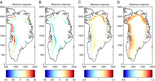
(A–D) The pattern of additional thickness change generated by enhanced lubrication by the CISM 2.0 model in (A) RUN0002 and (B) RUN1026 (mean for 2190–2199 differenced against SMBONLY) and pattern of velocity change again for (C) RUN0002 and (D) RUN1026 (expressed as ratio to SMBONLY velocity).

Discussion

Our model results show the widespread consequences of changes in meltwater-enhanced lubrication on the flow of the GrIS. Importantly, our results show that these changes have a minor (∼5%) effect on the overall contribution of the ice sheet to future SLR. Changes in the internal flow of an ice sheet alone do not necessarily affect its overall mass budget; they merely redistribute mass from one part of the ice sheet to another. For the overall ice-sheet mass budget to be affected one or both of the ice sheet’s two primary mass loss mechanisms, surface meltwater runoff or iceberg calving, must be altered. The mass-redistribution effect is clear in Fig. 5, where faster flow in the ice-sheet interior leads to local thinning and downstream thickening for both minimum and maximum parameterizations. The effect of the two parameterizations, however, differs near the margin: The maximum parameterization encourages continued flow to the margin, where ablation rates and mass loss are large, whereas the minimum parameterization retards flow to the margin with a consequent exaggeration in thickening. These changes in geometry will have further affected flow because of their influence in reducing ice-surface slope and therefore gravitational driving stress.

Our experiments specify SMB, so that altered mass loss by melt is not possible except directly at the ice margin (where annual negative SMB may be in excess of the marginal ice thickness). Alternatively, increased ice flow toward the calving fronts of outlet glaciers could affect mass loss. Our results for the overall effect of meltwater-enhanced lubrication on SLR show that these effects are small. In fact, there are several instances (in the first century of several experiments and in the second century of the minimum experiments) where mass delivery to the margin is reduced, leading to sea-level fall (relatively to SMB forcing only).

By specifying SMB, we omit one potential mechanism that could further affect net mass loss: the drawdown of faster-flowing ice leading to a lower ice surface that may then experience higher near-surface air temperatures and increased melt (the reverse process will clearly operate in the downstream areas that receive this additional mass flux). We tested this concept by repeating our experiments using the VUB-GISM-HO model with SMB determined interactively, using a degree-day model (DDM) (26). Experiments allowed DDM-derived SMB to evolve freely between 2000 and 2200 or held SMB fixed at its DDM-derived value for 2000. The difference between incorporating basal lubrication (RUN1026) or not (i.e., SMBONLY) was 6.5 mm SLR by 2200 for the freely evolving SMB run and 5.9 mm for the fixed SMB run. This suggests that the error introduced in our main experiment by holding SMB fixed is ∼0.6 mm, which confirms the relatively small influence of lubrication on the net mass loss from the GrIS. Alternatively this effect could be assessed by careful parameterization of the SMB-elevation feedback, as for example formulated by Helsen et al. (30).

It remains to assess how representative the climate forcing that we used is of the ensemble of projections for future Greenland climate. Fettweis et al. (17) show that the ECHAM5-forced MAR projections of SMB used here mirror the Coupled Model Intercomparison Project Phase 5 (CMIP5) multimodel mean for IPCC's Representative Concentration Pathway 8.5 (RCP8.5) scenario up to 2070 and then diverge to be ∼25% lower by 2100 (but still well within the intermodel range). This is also true for runoff projections. The Elmer/Ice simulations reported here show that HadCM3 forcing for A1B produced similar results to those discussed above, and E1 forcing has 40–50% of the effect of A1B forcing.

Overall, our results suggest that meltwater-enhanced basal lubrication can be important for the future contribution of the GrIS to SLR only if it interacts with mass loss, perhaps most likely by affecting increased iceberg calving. The modeling of this process presents numerous theoretical and technical challenges and has yet to be fully incorporated into the type of continental-scale ice sheet model used here. In the future, increasing quantities of surface meltwater may affect ice flow in other ways. For instance, the release of the meltwater’s latent heat may warm ice and therefore change its rheology (31) either at the bed or englacially.

References

- 1.Hubbard BP, Sharp MJ, Willis IC, Nielsen MK, Smart CC. Borehole water-level variations and the structure of the subglacial hydrological system of Haut Glacier d’Arolla, Valais, Switzerland. J Glaciol. 1995;41(139):572–583. [Google Scholar]
- 2.Zwally HJ, et al. Surface melt-induced acceleration of Greenland ice-sheet flow. Science. 2002;297(5579):218–222. doi: 10.1126/science.1072708. [DOI] [PubMed] [Google Scholar]
- 3.Alley RB, Clark PU, Huybrechts P, Joughin I. Ice-sheet and sea-level changes. Science. 2005;310(5747):456–460. doi: 10.1126/science.1114613. [DOI] [PubMed] [Google Scholar]
- 4.Das SB, et al. Fracture propagation to the base of the Greenland Ice Sheet during supraglacial lake drainage. Science. 2008;320(5877):778–781. doi: 10.1126/science.1153360. [DOI] [PubMed] [Google Scholar]
- 5.Catania GA, Neumann TA. Persistent englacial drainage features in the Greenland Ice Sheet. Geophys Res Lett. 2010;37(2):L02501. [Google Scholar]
- 6.van de Wal RSW, et al. Large and rapid melt-induced velocity changes in the ablation zone of the Greenland Ice Sheet. Science. 2008;321(5885):111–113. doi: 10.1126/science.1158540. [DOI] [PubMed] [Google Scholar]
- 7.Joughin I, et al. Seasonal speedup along the western flank of the Greenland Ice Sheet. Science. 2008;320(5877):781–783. doi: 10.1126/science.1153288. [DOI] [PubMed] [Google Scholar]
- 8.Bartholomew I, et al. Seasonal evolution of subglacial drainage and acceleration in a Greenland outlet glacier. Nat Geosci. 2010;3:408–411. [Google Scholar]
- 9.Bartholomew I, et al. Supraglacial forcing of subglacial drainage in the ablation zone of the Greenland ice sheet. Geophys Res Lett. 2011;38:L08502. [Google Scholar]
- 10.Bartholomew I, et al. Short-term variability in Greenland Ice Sheet motion forced by time-varying meltwater drainage: Implications for the relationship between subglacial drainage system behavior and ice velocity. J Geophys Res. 2012;117:F03002. [Google Scholar]
- 11.Price SF, Payne AJ, Catania GA, Neumann TA. Seasonal acceleration of inland ice via longitudinal coupling to marginal ice. J Glaciol. 2008;54(185):213–219. [Google Scholar]
- 12.Sundal AV, et al. Melt-induced speed-up of Greenland ice sheet offset by efficient subglacial drainage. Nature. 2011;469(7331):521–524. doi: 10.1038/nature09740. [DOI] [PubMed] [Google Scholar]
- 13.Schoof C. Ice-sheet acceleration driven by melt supply variability. Nature. 2010;468(7325):803–806. doi: 10.1038/nature09618. [DOI] [PubMed] [Google Scholar]
- 14.Parizek BR, Alley RB. Implications of increased Greenland surface melt under global-warming scenarios: Ice-sheet simulations. Quat Sci Rev. 2004;23(9-10):1013–1027. [Google Scholar]
- 15.Huybrechts P, De Wolde J. The dynamic response of the Greenland and Antarctic ice sheets to multiple-century climatic warming. J Clim. 1999;12(8):2169–2188. [Google Scholar]
- 16.Fettweis X. Reconstruction of the 1979-2006 Greenland ice sheet surface mass balance using the regional climate model MAR. Cryosphere. 2007;1(1):21–40. [Google Scholar]
- 17.Fettweis X, et al. Estimating Greenland ice sheet surface mass balance contribution to future sea level rise using the regional atmospheric climate model MAR. Cryosphere. 2013;7:469–489. [Google Scholar]
- 18. Rae J, et al. (2012) Greenland ice sheet surface mass balance: Evaluating simulations and making projections with regional climate models. Cryosphere 6:1275–1294.
- 19.Hewitt IJ. Modelling distributed and channelized subglacial drainage: The spacing of channels. J Glaciol. 2011;57(202):302–314. [Google Scholar]
- 20.Dee DP, et al. The ERA-Interim reanalysis: Configuration and performance of the data assimilation system. Q J R Meteorol Soc. 2011;137(656):553–597. [Google Scholar]
- 21.Bamber JL, Layberry RL, Gogineni S. A new ice thickness and bed data set for the Greenland ice sheet 1. Measurement, data reduction, and errors. J Geophys Res D Atmos. 2001;106(D24):33773–33780. [Google Scholar]
- 22.Le Brocq AM, Payne AJ, Siegert MJ, Alley RB. A subglacial water-flow model for West Antarctica. J Glaciol. 2009;55(193):879–888. [Google Scholar]
- 23.Bartholomew I, et al. Seasonal variations in Greenland Ice Sheet motion: Inland extent and behaviour at higher elevations. Earth Planet Sci Lett. 2011;307:271–278. [Google Scholar]
- 24. Cleveland WS, Grosse E, Shyu WM (1992) Local regression models. Statistical Models, eds Chambers JM, Hastie TJ (Wadsworth & Brooks/Cole, Pacific Grove, CA), Chap 8.
- 25.Huybrechts P. Sea-level changes at the LGM from ice-dynamic reconstructions of the Greenland and Antarctic ice sheets during the glacial cycles. Quat Sci Rev. 2002;21:203–231. [Google Scholar]
- 26.Goelzer H, et al. Sensitivity of Greenland ice sheet projections to model formulations. J Glaciol. 2013;59(216):733–749. [Google Scholar]
- 27. Gillet-Chaulet F, et al. (2012) Greenland Ice Sheet contribution to sea-level rise from a new-generation ice-sheet model. Cryosphere 6:1561–1576.
- 28.Price SF, Payne AJ, Howat IM, Smith BE. Committed sea-level rise for the next century from Greenland ice sheet dynamics during the past decade. Proc Natl Acad Sci USA. 2011;108(22):8978–8983. doi: 10.1073/pnas.1017313108. [DOI] [PMC free article] [PubMed] [Google Scholar]
- 29.Perego M, Gunzburger M, Burkardt J. Parallel finite-element implementation for higher-order ice-sheet models. J Glaciol. 2012;58(207):76–88. [Google Scholar]
- 30.Helsen MM, van de Wal RSW, van den Broeke MR, van de Berg WJ, Oerlemans J. Coupling of climate models and ice sheet models by surface mass balance gradients: Application to the Greenland Ice Sheet. Cryosphere. 2012;6:255–272. [Google Scholar]
- 31.Phillips T, Rajaram H, Steffen K. Cryo-hydrologic warming: A potential mechanism for rapid thermal response of ice sheets. Geophys Res Lett. 2010;37:L20503. [Google Scholar]
Associated Data
This section collects any data citations, data availability statements, or supplementary materials included in this article.