DBSI: DNA-binding site identifier

Abstract

In this study, we present the DNA-Binding Site Identifier (DBSI), a new structure-based method for predicting protein interaction sites for DNA binding. DBSI was trained and validated on a data set of 263 proteins (TRAIN-263), tested on an independent set of protein-DNA complexes (TEST-206) and data sets of 29 unbound (APO-29) and 30 bound (HOLO-30) protein structures distinct from the training data. We computed 480 candidate features for identifying protein residues that bind DNA, including new features that capture the electrostatic microenvironment within shells near the protein surface. Our iterative feature selection process identified features important in other models, as well as features unique to the DBSI model, such as a banded electrostatic feature with spatial separation comparable with the canonical width of the DNA minor groove. Validations and comparisons with established methods using a range of performance metrics clearly demonstrate the predictive advantage of DBSI, and its comparable performance on unbound (APO-29) and bound (HOLO-30) conformations demonstrates robustness to binding-induced protein conformational changes. Finally, we offer our feature data table to others for integration into their own models or for testing improved feature selection and model training strategies based on DBSI.

INTRODUCTION

Protein–DNA interactions play a pivotal role in many biological processes, such as gene regulation, DNA replication, recombination and repair. Although the biophysical principles that determine selective protein–DNA binding are not entirely clear, effective models for prediction of DNA-binding sites can shed light on the basic mechanisms for recognition.

Many distinct methods have been developed to predict DNA-binding residues on a protein surface (1–22). Some of these are based on the primary sequence of a protein (4,7,9,10,12,15–18,21), whereas others are built using structure-based information (1,2,5,6,8,11,13,14,19,20,22). Machine-learning methods such as support vector machine (SVM) classifiers (15,19), neural networks (1,13) and random forest-based approaches (16,18) have been used for training feature-based models to identify DNA-binding sites.

Sequence-based methods make predictions using properties derived from information such as the position-specific scoring matrix (23), sequence conservation (24), amino acid frequency (25), predicted secondary structure (10), predicted solvent accessibility (10) and the BLOSUM62 matrix (7). In contrast, structure-based methods use properties such as electrostatic potential (8), protein surface shape (14), secondary structure (1,21), amino acid microenvironment (3,13) and relative solvent accessible surface area (SASA) (21). In addition, the biochemical characteristics of amino acid side chains are important properties for characterizing DNA-binding sites (3,8,26–30). Finally, some methods combine information derived both from structural data and evolutionary information. Using global protein structural alignments and statistical potentials, Gao et al. (5) developed a knowledge-based method for predicting DNA-binding proteins and their binding sites. Ozbek et al. (11) developed a method to predict DNA-binding residues based on evolutionary conservation and the fluctuation of side chains in high-frequency Gaussian normal modes.

In this study, we introduce the DNA-Binding Site Identifier (DBSI), a structure-based method for identifying DNA-binding sites on proteins that are known or believed to bind DNA. Starting with 480 features, including a number of electrostatics features unique to our model, DBSI was developed by optimizing the feature combination and training parameters via a forward selection iterative approach. Our results suggest that DBSI can predict DNA-binding sites reliably, based on cross-validation analysis on 263 training examples and testing on 206 independent examples. In addition, by studying proteins with both bound and unbound structures, we demonstrate that DBSI can predict DNA-binding sites starting from the unbound structure with similar accuracy to predictions made using the bound protein structure. This is a significant observation, as prediction on unbound structures is the expected starting point in practical applications. We present rigorous comparisons with established methods, including DISPLAR and the consensus predictions of metaDBsite (12), which are based on compilation of individual predictions of DBS-Pred (1), DP-Bind (7), DISIS (10), BindN/BindN-rf (16,17) and DNABindR (21). The comparative results establish a clear predictive advantage of DBSI in comparison with these outstanding existing methods. DBSI also develops several new electrostatics-based features that are both unique to our work and inspired by past observations on the importance of electrostatics to protein–DNA recognition (3,8,26–30).

MATERIALS AND METHODS

Training and validation data

Several data sets were used in this study. The training data set comes from Tjong et al.’s article (13), in which 264 proteins were used to train the DISPLAR model. We used 263 complexes from their article, excluding one (PDB ID: 1MJE), which had too many fragments missing in the protein–DNA complex to be a reliable training example. This data set contains one spurious protein–RNA interface (PDB ID: 1U1Y), whereas the remaining 262 examples are protein–DNA complexes. The PDB codes for this training data set (TRAIN-263) are given in Supplementary Table S1. This data set contains examples with up to 50% sequence identity. To avoid training bias, examples with >25% sequence identity or sharing a common fold were grouped together when performing cross-validation, as described in ‘Evaluation of Model Performance’ section

Our test data contain 206 examples compiled from the data set of metaDBsite (12). The metaDBsite consensus server was trained on a data set of 316 examples. Of these, 219 chains from 206 PDB files are distinct from the examples in our training data set. We used this data set (TEST-206) as an added test set for comparison between methods. For this data set, we report aggregate performance as well as performance relative to sequence similarity with examples in our training data.

Finally, we compiled bound and unbound structures for DNA-binding proteins having low sequence identity to examples in the TRAIN-263 data set. These examples were derived from the articles of both Ozbek and Xiong (11,19). Ozbek compiled 54 pairs of structures, which included both protein–DNA complexes (HOLO) and unbound proteins (APO). One of the HOLO complexes (PDB ID: 1I6H) contains >2000 residues and was deleted from our test data set because predictions on this example would exert too much influence on the combined statistics for the predictive results. Three additional APO proteins were deleted as well, as two have only CA traces (PDB IDs: 1LRP and 1BGT), and the third corresponds to 1I6H (PDB ID: 1NIK), which was deleted from our APO data set owing to its large size. For the remaining 53 bound protein–DNA complexes and 50 unbound proteins, we used the PISCES server (31) to calculate the homology score between these proteins and the proteins in the TRAIN-263 data set. Of these, we identified six HOLO protein–DNA complexes and five APO proteins having a sequence identity of <25% with examples in our training set. Xiong used 83 protein–DNA complexes (HOLO-83) and 83 unbound proteins (APO-83) as their test data, and using the same procedure, we obtained an additional 24 protein–DNA complexes and unbound proteins. All together, we identified 30 protein–DNA complexes for use in our bound test data set (HOLO-30), for which 29 had available unbound structures suitable for use in our unbound test data set (APO-29). The remaining unbound example (PDB ID: 1LRP) contained only a CA trace. PDB codes for all data sets are available in Supplementary Table S1. Supplementary Table S2 also contains results for alignments between the APO and HOLO examples. Using TM-align (32), the root mean square deviation (RMSD) calculation is reported for aligned subregions, the full CA RMSD calculations based on these alignments and the CA RMSD of surface interface and non-interface residues. In addition, backbone and all-atom RMSD values of aligned subregions are reported for the best alignments obtained using PyMOL (33). For the full CA RMSD based on the TM-align alignment, computed RMSD values ranged from 0.45 to 24.38 Å, with a median of 1.73 Å, a mean of 4.54 Å and a standard deviation of 6.89 Å. For surface residues in the protein–DNA interface, the RMSD values ranged from 0.18 to 29.31 Å with a median of 1.64 Å, a mean of 4.53 Å and a standard deviation of 7.08 Å. For surface residues outside the protein interface, values ranged from 0.39 to 27.15 Å, with a mean of 1.61 Å, a median of 4.89 Å and a standard deviation of 7.33 Å. These values show that non-trivial conformational changes occur between the apo and holo structures, and that these changes occur both for interface and non-interface residues.

Surface residues were defined as those with relative SASA (defined as observed SASA compared with maximum possible within an ALA-X-ALA tripeptide) of at least 10%, as calculated by NACCESS (34). A surface residue was classified as a DNA-binding residue if the distance between any of its heavy atoms and a heavy atom of DNA was within 5.0 Å. Based on this definition, the TRAIN-263 data set contains 56 325 surface residues, with 18% positive (DNA binding) and 82% negative (non-DNA binding) examples; the TRAIN-206 data set contains 38 666 surface residues, with 16% positive and 84% negative examples; the HOLO test data set contains 7568 surface residues, with 13% positive and 87% negative examples; the APO test data set contains 6777 surface residues, with 12% positive and 88% negative examples.

Evaluation of model performance

To avoid overfitting the training data, we applied both standard leave one residue out cross-validation and 10-fold cross-validation. For the 10-fold cross-validation, we divided the TRAIN-263 data set into 10 different groups; proteins in nine groups were used to train models, and the proteins in the remaining group were used to test the models. To avoid bias due to evolutionary relationships between the training examples, proteins having sequence identity >25% as determined using PISCES (31) were assigned to the same group. Despite this sequence identity threshold, proteins of a given tertiary structure may exhibit a high degree of sequence variation. As a further step to reduce training bias, TM-align (32) was used to perform pairwise structural alignments on proteins of the TRAIN-263 set. Proteins with a TM-score exceeding 0.3 were placed into the same cross-validation group.

Because our data set contains more negative examples than positive examples, overall accuracy is heavily biased by the accuracy in predicting negative examples. To provide a full characterization of predictive ability, several other parameters are also used to evaluate the performance of DBSI. These are ‘Sensitivity’, ‘Specificity’, ‘Precision’, ‘Accuracy’, ‘F1 Score’, ‘Strength’ and ‘Matthews Correlation Coefficient’, defined as follows:

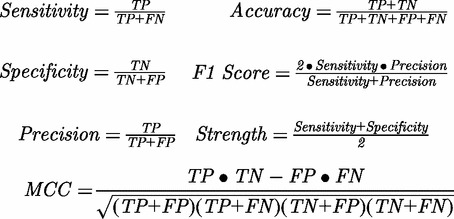Here, TP is the number of true positives; TN is the number of true negatives; FP is the number of false positives; and FN is the number of false negatives. ‘Sensitivity’ is the accuracy for positive examples, ‘Specificity’ is the accuracy for negative examples, ‘Precision’ is the accuracy for all predicted positive examples, ‘F1 Score’ is a combination of Sensitivity and Precision, and ‘Strength’ is the average of Sensitivity and Specificity. These additional parameters, along with MCC, provide a good complement to Accuracy, which is easily biased in the case where there is an imbalance between positive and negative examples in the training or testing data sets.

In addition to these measures, the Area under the Curve (AUC) of the Receiver Operating Characteristic (ROC) curve is a useful metric for assessing predictive performance. The ROC curve shows the relationship between the true positive rate (Sensitivity) and the false positive rate (1.0-Specificity) as the cutoff score for distinguishing positive and negative examples is adjusted. The cutoff is varied from its lowest possible value (all examples are predicted as positive examples, hence Sensitivity = 1 and Specificity = 0) to its highest possible value (Sensitivity = 0 and Specificity = 1). The AUC indicates how strongly the data are classified. For example, a bimodal distribution for which all positive examples were classified with score 1.0 and all negative examples with score −1.0 would achieve an AUC of 1.0. In a real setting, some classification scores will be nearer to zero, and some examples will be misclassified. Models with AUC < 0.5 are considered to be poor models, whereas acceptable models typically have AUC > 0.7 and more highly predictive ones AUC > 0.8, with values of AUC > 0.9 being challenging to achieve in practice.

Model training and feature selection. Different learning methods such as Neural Networks (1,13), Random Forests (16,18) and SVM, have been used for training models to predict DNA-binding sites. In creating the DBSI model, we used the SVM^light program (35) in conjunction with a collection of 480 features outlined later in the text. SVM finds a set of hyperplanes able to classify two different classes of data with the largest margin, and it demonstrates high-predictive accuracy while avoiding over-fitting. Here, the surface residues in contact with DNA are considered as positive examples, and the surface residues that do not contact DNA are considered as negative examples. In addition to SVMs, we also tried training models using Random Forest (36) and decision trees (37), but we determined that models built by SVMs according to our iterative feature selection process, described later in the text, gave the highest predictive accuracy. The model development process occurred in three stages: feature selection using 1000 data points, SVM parameter selection using 6000 data points and full training and validation on the entire data set of over 50 000 data points. The sets of 1000 and 6000 examples were defined with 18% positive examples and 82% negative examples, mirroring their frequencies within the full training data set. This strategy was useful both to help speed the model training process and to guarantee that our model features and parameters were not overly biased toward good performance on the full training data set.

SVM kernel functions and parameters. We applied different SVM kernel functions (which transform the data before deriving hyperplanes), such as polynomial kernels and Gaussian kernels. The Gaussian kernels were found to provide the best improvements over linear SVM. For the Gaussian kernels, several parameters can be tuned to obtain the highest accuracy. The parameter C controls the trade-off between allowing training errors and enforcing rigid margins; the parameter G determines the Gaussian width; another parameter J is a cost factor, by which training errors on positive examples outweigh errors on negative examples. In optimizing the DBSI model, we tested C values from 0.0 to 64.0, G values from 0.0 to 2.0 and J values from 2.0 to 6.0.

Iterative feature selection. Because we had a large number of features as well as a large data set, it was important to devise some strategy for feature selection. The use of Random Forests (36) built using decision trees is a common approach to feature selection. There are additional strategies that apply a range of techniques, which often attempt to prune the collection of features in one manner or another (38–40). However, our collection of features is large; therefore, we attempted a ‘bottom up’ rather than ‘top down’ approach to feature selection.

To speed the feature selection process, 1000 randomly chosen data points from TRAIN-263 were used to identify features with good predictive value for training the DBSI model. First, the features were divided into general categories, e.g. electrostatics, position specific scoring matrix (PSSM), microenvironment. We then trained models on the reduced training set using individual features (or PSSM feature groups.) Next, we trained a model by combining the best individual features, then iteratively adding successive additional features. With each iteration, we included an additional feature (or PSSM feature group) and then retrained the model. The resulting best model (in F1 Score) from one iteration became the starting point for the next iteration. We terminated the feature selection process once the F1 Score could no longer be improved. Features within the electrostatics and PSSM categories were found to have the best predictive value; therefore, our starting model for the iterative feature selection process was the best one that could be built by combining a single electrostatics feature and a single PSSM feature group.

Parameter refinement and cross-validation. Using the best feature combination from our iterative selection process, we optimized the SVM training parameters on an expanded data set of 6000 randomly selected training examples. The final DBSI model was then trained and cross-validated on the entire training data set.

Features used in training the DBSI model

We generated several different types of features (both structure-based and sequence-based) for identifying DNA-binding sites. A complete list of 480 features used in our study is given in Supplementary Table S3, and the numbers assigned to the features in this table are given in listings of the feature groups. Later in the text, we describe each feature category and key details of the calculations. The listing of features is divided into groups, so as to avoid having the discussion be too dense. Roughly, Features 1–13 describe simple features that can be defined at the residue level using lookup tables or standard calculations. Features 14–180 are derived for each residue based on properties of neighboring residues and/or calculations using grid-based local environments. Features 181–480 are simply PSSM matrices with different window sizes.

Residue characteristics (Features 1–4). Three simple residue characteristics were used as features for this study: hydrophobicity, size and charge. The Fauchere and Pliska hydrophobic scale was used to express the hydrophobicity of side chains (41). Residue size was characterized by the maximum SASA within a ALA-X-ALA tripeptide (42). This feature is a constant value independent of the residue’s context within a protein structure and is thus different than the value calculated described in the SASA-based features. ARG and LYS were assigned a charge of +1, ASP and GLU a charge of −1, HIS a charge of +0.5, and all other residues a charge of 0.

A new feature called pseudo hydrophobicity was generated based on the combination of hydrophobicity and charge. If the charge of the residue was non-negative, the pseudo hydrophobicity was defined as the hydrophobicity of the residue; if the charge of the residue was negative, the pseudo hydrophobicity was defined as the product of the hydrophobicity index and the charge of the residue.

Secondary structure (Features 5 and 6). Secondary structure assignments were made with DSSP (36,37), which classifies protein residues as one of nine different types: alpha helix (H), residue in isolated beta-bridge (B), extended strand participates in beta ladder (E), 3-helix (or 3₁₀ helix) (G), 5-helix (or pi-helix) (I), hydrogen-bonded turn (T), bend (S), loop (L) and irregular (no designation). Across the entire training data set, each surface residue was assigned, and the probability distribution of secondary structure types was tabulated along with the probability distribution for just the DNA-binding residues. The ratio of probabilities for the binding residues and all surface residues were calculated for each secondary structure type. This results in a numerical value for each secondary structure classification, reflecting its propensity to exist a protein–DNA interface. Also, a simple secondary structure feature assigned a value of +1 to residues in an extended strand (E), −1 to residues in an alpha helix, and 0 to all other residues.

SASA (Features 7–12). SASA was calculated by the program NACCESS (34). The relative SASA of each residue is calculated by using the corresponding SASA of the tripeptide (ALA-X-ALA) as a reference. The relative SASAs of the entire residue and the residue’s side chain defined two features. Polar SASA, the relative polar SASA, non-polar SASA and the relative non-polar SASA were considered as four other features related to SASA. The polar SASA is the total SASA of all oxygen and nitrogen in the side chain, and the non-polar SASA is the total SASA of all other of atoms in the side chain.

Polar atom availability (Feature 13). In a given side chain, the availability of O and N atoms for participation in hydrogen bonds was used as a feature. For example, in the ARG side chain, there are three polar nitrogens. If N of these atoms are making internal hydrogen bonds, the feature value is set to 3-N. In general, the value of the feature is the number of polar side chain atoms not involved in internal hydrogen bonds.

Electrostatic potential (Features 14–41). We used the PBEQ-Solver (43,44) to calculate the electrostatic potential of proteins using the CHARMM-GUI (45). The PBEQ-Solver can be used to calculate protein electrostatic potential and solvation energy, protein–protein electrostatic interaction energy and pKa of a titratable residue. We also explored the use of APBS (46) in training and testing our models, finding that calculations based on PBEQ produced models with a somewhat higher true-positive rate; however, as APBS is a popular and more automatable option for electrostatics calculation, we provide scripts for APBS that reproduce as closely as possible the calculation we performed using PBEQ.

Several parameters must be specified when solving the Poisson–Boltzmann equation using the PBEQ-Solver, such as the dielectric constant for the protein interior, the solvent dielectric constant, salt concentration, the grid spacing in the finite-difference and the distance between a protein atom and a grid point. We used all PBEQ default values except for the assignment of the dielectric constant for the protein interior (2.0), the coarse finite-difference grid spacing (1.0 Å) and the fine finite-difference grid spacing (0.5 Å). Values on the fine grid were used for all described calculations.

At each atom, the electrostatic potential of nearby grid points was averaged to create an atomic-scale electrostatic feature. Local averaging of the electrostatic potential at grid points between the van der Waals and solvent accessible surfaces was performed, using a solvent probe radius of 1.4 Å. For each atom, values for the electrostatic potential at grid points were averaged at grid points outside the protein’s van der Waals surface but within a distance that is the sum of the atom radius and the solvent radius. Three additional groups of features (seven features/group) were derived by moving the shell slightly outward, by radius offsets 0.1, 0.3 and 0.5 Å. The region of the shell maintains a width of 1.4 Å, regardless of the offset, but the regions move farther away from the van der Waals surface as the offset is varied. Mathematically, this is equivalent to adding the offset value to the radius of all the atoms and repeating the previous calculation described for the van der Waals and solvent accessible surfaces. Figure 1 illustrates the details of this calculation at the atom level. Figure 2 illustrates the change in residue level features as the surface offset is increased.

Figure 1.

The figure illustrates calculation of the atom-level electrostatic feature within a shell offset 0.5 Å from the van der Waals surface. The grid on which the electrostatic potential is calculated is shown relative to the molecule, shown in dark gray, and the atom at which the feature is calculated is marked using a black dot. Electrostatic potential values at grid points within the light gray annular region are those averaged to generate the feature for this atom. Grid points inside the 0.5 Å offset surface are excluded from the calculation. The light gray annular region is 1.4 Å in width, regardless of the offset used to define the shell.

Figure 2.

The basic residue-level electrostatics feature is mapped onto the surface of the Nucleosome Core Particle (PDB 1KX5). The feature calculated in the shell between the van der Waals and solvent accessible surface (top) shows patches where this feature takes on negative values. When this feature is calculated for the shell that is shifted 0.5 Å outward, some patches flip from negative to positive. Thus, a region that might otherwise seem unfavorable to DNA binding is now seen to have the correct biophysical characteristics for recognition.

Next, we derived local sums and averages of the residue-level electrostatic features in the neighborhood of the target residue. The sum was taken at neighboring residues within 7 Å of the target residue, and sums that both included and excluded the target residue were used as features. In addition to the sums, the average values were also used as features. Finally, values for each target residue electrostatic feature (described in the previous paragraph) were ordered from lowest to highest and normalized by the sequence length within each protein, which defines a relative electrostatics feature with values between 0 and 1. The same calculation was applied to the average value at neighboring residues (excluding the target residue) as described earlier in the text, to define a relative electrostatics feature in the local environment surrounding the residue. Thus, each residue-level electrostatic feature generates six additional features that are derived from it based on local sum/average and normalization.

Surface curvature (Features 42–48). We used the residue-level curvature values as reported by the program SURFCV (47) as features. We also derived local sums and averages, both including and excluding the target residue, using calculations similar to those described for the electrostatic potentials. We also derived the normalized ranked values for the residue curvature and the neighbor average curvature feature, again following the calculations described in the previous section.

Local atomic density (Features 49–98). Local atomic density has been used as a feature to predict hot spots in our previous works (48–50). In this study, we tested features related to local atomic density to determine their effect on prediction of DNA-binding sites. Using Fast Atomic Density Evaluator (FADE) (51), a 3D grid of points surrounding the protein was generated. Grid points whose distance to the molecule is <3 Å is a FADE point. At each FADE point, a shape score is also generated. These calculations can detect knobs and holes at the residue-scale, whereas the previously described curvature calculations can identify larger scale features, such as the saddle shapes of protein–DNA interfaces.

A 10 Å sphere, divided into nested 1 Å shells, is placed at the (geometric) center of each target residue. Within each shell, a feature is defined by adding all the shape values for FADE points within that shell. This produces 10 features. A second group of 10 features normalizes the shape features values by the volumes of their respective shells. The number of FADE points within each shell comprises another group of 10 features. This group of features is also normalized by the shell volume to produce an additional set of 10 features. Finally, Z-scores for these normalized features produced an additional 10 features.

Residue microenvironments (Features 99–164). In addition to the locally averaged shape and electrostatic features defined previously, several groups of features based on local microenvironments were defined. In the first case, a distance cutoff equal to 5 Å using all residues was applied, and the second definition used a distance cutoff equal to 7.0 Å applied only to surface residues. The following residue microenvironment features were calculated: the total number neighboring residues, the total number of individual amino acid neighbors, the total charge, the total hydrophobicity, the total number of rotatable single bonds and the total number of weighted rotatable single bonds. Several of these features were used in our KFC2 hot spot model (50).

We also calculated the total secondary structure values and the total secondary structure similarity values of the neighbor residues. First, scores of −1.0, 1.0 and 0.0 were assigned to residues with ‘H’, ‘E’ and all other secondary structure types, respectively (Feature 2). Combined secondary structure values of neighbor residues were calculated according to the microenvironment definitions. A secondary structure similarity score between the target residue and neighbor residues was also derived. For example, if the secondary structure value of the target residue was the same as one of the neighbor residues, their similarity score was set to 1.0; otherwise, the similarity score was 0.0. Using this definition, we calculated the total similarity score between the target residue and neighbor residues.

Finally, normalized values for several of these features, obtained by dividing the features by the number of neighboring residues, were used as additional features.

Non-local polar and electrostatic microenvironments (Features 165–180). In addition to the local microenvironments defined by neighboring residues, we examined the use of features defined within two distance bands that are relevant to DNA binding. In the canonical DNA B-conformation, the two neighboring phosphates and base pairs are separated by specific distances. If a DNA-binding residue is involved in a hydrogen bond with DNA, there is greater likelihood in finding another H-bond donor at an appropriate spacing able to facilitate a second hydrogen bond. Based on this hypothesis, we created two features by counting residues whose H-bond donors are within a certain distance of a H-bond donor in the target residue, using distance bands of 5–8 Å and 11–14 Å. The latter distance is comparable in scale with the width of the B-DNA minor groove.

We performed a similar calculation for electrostatic features in the same distance bands, starting from the basic residue-level electrostatic feature (Feature 14), to derive additional non-local electrostatic microenvironment features. As with the other electrostatic features, sums, averages and normalized rank features were generated. Features were generated both by including and excluding the target residue when performing the calculation.

PSSM (Features 181–480). Our PSSM features were derived from multiple sequence alignments generated by PSI-BLAST (52), using the NCBI non-redundant database (53), dated October 16 16:36:39 2011. The search was limited to three iterations with e-value threshold 10⁻³, which is the same calculation used by DISPLAR (13). These are the only sequence-based features used in our model, accounting for 300 of 480 features. These features cannot be added independently of one another but must be added in groups.

Each group of features is a subset of the PSSM matrix for a short window of residues, containing log likelihood scores for each of the 20 amino acids at each position of the window. Thus, if we have a target residue and are looking at 3 residues on either side of this target residue, the window has length 7, and the total number of features (corresponding to the entries of the PSSM matrix) is 140. We generated the feature groups using various window sizes having 2–7 flanking residues on each side of the target residue, based on the multiple sequence alignments as described earlier in the text. The values of the PSSM features do not change as we change the window size. The PSSM values are entirely determined from the multiple sequence alignment, and only the number of PSSM features changes with the window size.

RESULTS

Feature selection and predictive ability

As described in the ‘Introduction’ section, other works have explored the use of features based on electrostatics, PSSM and the distribution of specific amino acids as important predictive features. For this reason, we paid special attention to these categories of features, first doing individual feature analysis on these categories of features, from which we began our iterative feature selection process. We note that the PSSM features are standard calculations that have been used in other works, and the amino acid microenvironments are based on simple calculations. The electrostatic features, on the other hand, are our own novel constructs that have not appeared in prior work. They exhibit interesting behavior near the protein surface, and they factor strongly into the predictive accuracy of our model.

Predictive accuracy of electrostatic features. We calculated features based on the electrostatic potential within different shells near the protein surface, as described in the ‘Materials and Methods’ section. Because these features had not been used in our own or previous works, we were interested to determine the quality of models that could be obtained by using them as individual features. The models were trained on the 1000 random subset used for feature selection, and the results reported represent the statistics for training parameters resulting in the best F1 Score using leave-one-out cross-validation, which may be different according to the specific feature. Also, these are not intended as highly predictive models, and thus they have much lower accuracy than DBSI; instead, this analysis is meant to suggest relative differences between the individual features on small subsets of the training data, which helps guide our feature selection process.

Table 1 shows results for single feature analysis for four of the electrostatic features in each shell. The pattern of behavior is interesting as the shells move away from the protein surface. For the features calculated using electrostatic potentials within the first shell, between the van der Waals and solvent accessible surface, the Sensitivity is low (0.06–0.16), but the Specificity is high (0.96–0.99). Thus, although the false-positive rate is remarkably low, these features result in few true-positive predictions. Predictions in the next shell, which is 1.4 Å in width but 0.1 Å outside the van der Waals surface, exhibit similar ranges for Sensitivity (0.08–0.18) and Specificity (0.97–0.99).

Table 1.

The best model for each electrostatic feature on a subset with 1000 data points

Electrostatic feature	Sensitivity	Specificity	Precision	F1
ESP_T (Feature 14)	0.06	0.99	0.63	0.10
AVE_ESP (Feature 17)	0.10	0.98	0.63	0.26
AVE_ESP1 (Feature 18)	0.10	0.98	0.53	0.17
RANK_AVEESP1 (Feature 20)	0.16	0.96	0.44	0.23
ESP_T_0.1 (Feature 21)	0.08	0.98	0.54	0.14
AVE_ESP_0.1 (Feature 24)	0.13	0.98	0.55	0.21
AVE_ESP1_0.1 (Feature 25)	0.09	0.99	0.59	0.16
RANK_AVEESP1_0.1 (Feature 27)	0.18	0.97	0.53	0.27
ESP_T_0.3 (Feature 28)	0.25	0.87	0.31	0.28
AVE_ESP_0.3 (Feature 31)	0.25	0.88	0.31	0.28
AVE_ESP1_0.3 (Feature 32)	0.30	0.88	0.35	0.32
RANK_AVEESP1_0.3 (Feature 34)	0.22	0.93	0.42	0.29
ESP_T_0.5 (Feature 35)	0.33	0.88	0.38	0.35
AVE_ESP_0.5 (Feature 38)	0.23	0.97	0.60	0.33
AVE_ESP1_0.5 (Feature 39)	0.31	0.94	0.54	0.40
RANK_AVEESP1_0.5 (Feature 41)	0.26	0.94	0.47	0.33

The number of the feature, as listed in Supplementary Table S3, is given in parentheses. Models were trained on the individual features related to electrostatics, in search of individual features with high predictive value. Predictive value in this case was measured using the F1 Score, which favored models having high Specificity but low to moderate Sensitivity. The best results were obtained for features calculated using the shell between the surfaces offset 0.5 Å from the van der Waals and solvent accessible surfaces. Based on this observation, we later checked whether use of more distant surfaces improved our final model, but this was not the case. The predictive value of the models trained on these individual features has F1 Scores that are fairly low, but in combination with other features, we will derive significantly better models.

As the bands move outward from the surface of the protein, the behavior transitions sharply. When the shell is offset 0.3 Å beyond the van der Waals surface, the Sensitivity jumps (0.22–0.30), whereas the Specificity drops somewhat (0.87–0.93). At the farthest shell, with offset 0.5 Å, Sensitivity continues to improve (0.23–0.33), and the Specificity increases relative to its previous drop (0.88–0.97).

The best F1 scores of models obtained for individual electrostatic features in various shells were 0.26, 0.27, 0.32 and 0.40, moving outward. This implies that features calculated in the more distant shells have higher predictive value, at least as individual features. We tested slightly more distant shells in training the final DBSI model to ensure additional improvements were not possible, and there was no improvement over those obtained using shells with offset 0.5 Å.

Predictive accuracy of PSSM features. PSSM matrices for window sizes 5, 7, 9, 11, 13 and 15 were assessed as feature groups, again using 1000 random training examples and leave-one-out cross-validation. It is not possible to assess PSSM features individually, as the size of the feature group is 20 times the window size. Table 2 suggests that the best predictive accuracy is obtained using a window size of 11. Unlike the electrostatic features, in which there was a significant difference among the features, the PSSM feature groups generated fairly similar results for the various window sizes. The lowest F1 Score occurs for PSSM[i − 2, i + 2], which has a window size of 5 and returns Sensitivity = 0.29, Specificity = 0.89 and F1 = 0.32. The highest F1 Score is for PSSM[i − 5, i + 5] with Sensitivity = 0.32, Specificity = 0.93 and F1 = 0.40. The performance of this model is roughly comparable with that of the best single feature electrostatic model. However, in combining these distinct predictive features, we expect to train a model that achieves a better predictive accuracy.

Table 2.

The best models for PSSM-based features based on a subset with 1000 training data points

PSSM features	Sensitivity	Specificity	Precision	F1
PSSM[i − 2, i + 2]	0.29	0.89	0.37	0.32
(Features 281–380)
PSSM[i − 3, i + 3]	0.28	0.93	0.48	0.35
(Features 261–400)
PSSM[i − 4, i + 4]	0.30	0.94	0.54	0.38
(Features 241–420)
PSSM[i − 5, i + 5]	0.32	0.93	0.52	0.40
(Features 221–440)

The feature numbers, as listed in Supplementary Table S3, are given in parentheses. These groups are nested so that the second group contains the first, and so on, up to the last group, which consists of all PSSM-based features. The predictive performance was comparable among the different groups, and although the inclusion of larger scoring windows improved performance somewhat, the improvement was statistically insignificant.

Predictive accuracy of residue microenvironment features. To assess the overall value of features related to local distribution of specific amino acids, we trained a model using these as a feature group, again using the 1000 data points used for the electrostatics and PSSM features. Table 3 shows a comparison of the best electrostatic, PSSM and microenvironment models. Remarkably, our best single electrostatic feature performs significantly better than the best model created with the 20 different microenvironment features, as does the PSSM[i − 5, i + 5] feature group. The microenvironment model achieves Sensitivity = 0.24, Specificity = 0.85 and F1 = 0.26, whereas both the electrostatics and PSSM models have F1 = 0.40 and higher Sensitivity and Specificity values.

Table 3.

Feature comparison and selection based on a subset with 1000 data points

Feature	Sensitivity	Specificity	Precision	F1
AVE_ESP1_0.5	0.31	0.94	0.54	0.40
(Feature 39)
Local Amino Acid	0.24	0.85	0.27	0.26
Microenvironment
(Features 133–152)
PSSM[i − 5, i + 5]	0.32	0.93	0.52	0.40
(Features 221–440)

Training results for best electrostatic-based feature (Table 1), best PSSM-based feature group (Table 2), and best residue microenvironment feature group are compared.

Feature selection and SVM parameter optimization. Using the iterative procedure described in the ‘Materials and Methods’ section, based on 1000 random training examples, we first looked for the best model that used only a single electrostatic feature and PSSM group. From this, we arrived at our starting model with a feature combination consisting of PSSM[i − 3, i + 3] and NEAR_ESP1_0.5 (Table 4). The first feature is the PSSM matrix with window size 7, and the latter is the total electrostatic potential at grid points near the target residue in the shell at offset 0.5 Å, including the target residue.

Table 4.

Progressive feature combinations used to develop DBSI

Iteration	Feature combination	Sensitivity	Specificity	Precision	F1
1	NEAR_ESP1_0.5	0.41	0.92	0.53	0.47
	PSSM[i − 3, i + 3]
	(Features 37, 261–400)
2	NEAR_ESP1_0.5	0.41	0.94	0.60	0.49
	PAA
	PSSM[i − 3, i + 3]
	(Features 13,37, 261–400)
3	NEAR_ESP1_0.5	0.41	0.95	0.63	0.50
	NEAR_ESP_0.3
	PAA
	PSSM[i − 3, i + 3]
	(Features 13,29,37, 261–400)
4	NEAR_ESP1_0.5	0.43	0.95	0.63	0.51
	NEAR_ESP_0.3
	PAA
	nnear_PTN
	PSSM[i − 3, i + 3]
	(Features 13,29,37, 175,261–400)

Based on the best combination of NEAR_ESP1_0.5 and the PSSM features, we successively introduced additional features. Descriptions of all features are in Supplementary Table S3.

Next, we applied the iterative procedure, as described in ‘Materials and Methods’ section, until the F1 Score converged. From all converged models, we identified the best feature combination in this study, which contains the following 164 features: NEAR_ESP_0.3, NEAR_ESP1_0.5, Polar Atom Availability (PAA), nRN1-nRN20, PSSM[i − 3, i + 3] and nnear_PTN. In Supplementary Table S3 and Table 4, these are given, respectively, as Features 13, 29, 37, 133–152, 175 and 261–400. The iterative process selected the single feature nRN11, corresponding to local LEU microenvironment, but we added the other 19 amino acids as a feature group. In the ‘Discussion’ section, we revisit the definition of these parameters and the possible biological reasons why they have predictive value toward prediction of DNA-binding sites.

After identifying the best feature combination, we wanted to determine the best C parameter, G parameter and J parameter for the final model. Because our training data set was so large, we randomly selected 6000 examples on which to optimize these parameters. We used leave-one-out cross-validation using different values of the C parameter (0.0–64.0), G parameter (0.0–2.0) and J parameter (0.0–6.0). The cross-validation produced the best results using parameter values C = 0.4, G = 0.0008 and J = 4.0 on this subset of 6000 training examples. These parameters were then used to train the final DBSI model on the entire training set of >50 000 training examples, on which a 10-fold cross-validation was performed to assess predictive performance.

Validation on training and independent data. Having established the best feature combination and the best kernel parameters, we applied 10-fold cross-validation to test the final DBSI model (although parameters were optimized using leave-one-out cross-validation on a small random subset of the training data, the validation of the model on the full training set is based on using 10-fold cross-validation. This is because there can be interdependencies within a protein interface, and removing only one residue from the full training data in cross-validation increases the likelihood that there is a highly related example that will bias the prediction, such as in the case of a protein dimer). DBSI achieved Sensitivity = 0.70, Specificity = 0.85, Precision = 0.50, Accuracy = 0.82, F1 = 0.58, Strength = 0.77 and MCC = 0.48 from applying this validation procedure to the TRAIN-263 data set. Performance on the TEST-206 independent data set was similar, returning Sensitivity = 0.74, Specificity = 0.85, Precision = 0.49, Accuracy = 0.83, F1 = 0.59, Strength = 0.80 and MCC = 0.51.

On the independent HOLO-30 data set of bound protein structures, DBSI achieved Sensitivity = 0.60, Specificity = 0.89, Precision = 0.45, Accuracy = 0.85, F1 = 0.52, Strength = 0.75 and MCC = 0.44. On the APO-29 data set of unbound protein structures, it achieved Sensitivity = 0.58, Specificity = 0.89, Precision = 0.42, Accuracy = 0.86, F1 = 0.48, Strength = 0.73 and MCC = 0.41. Significantly, this demonstrates a similar performance on unbound and bound protein structures, which need not be true for all methods incorporating structure-based features. The Sensitivity was lower for these data sets in comparison with the TRAIN-263 and TEST-206 data sets. However, these data sets are considerably smaller than the others and do not represent an exhaustive test; instead, the point of using these data sets was to compare performance on bound and unbound protein structures.

Figure 3 shows the ROC curve for TRAIN-263, TEST-206, APO-29 and HOLO-30. The AUCs for DBSI on these data sets were 0.86, 0.88, 0.83 and 0.85, respectively. These validation results are also summarized in Table 5. The next section will give comparisons between our results and those of established methods, and the ‘Discussion’ section will review features of the final model in greater detail.

Figure 3.

The ROC curves of the TRAIN-263, cross-validation results, along with the TEST-206, HOLO-30 and APO-29 predictions. In each case, the AUC is greater than 0.8, which indicates that DBSI is a highly predictive model.

Table 5.

Predictive performance of DBSI on the training and independent data sets relative to a variety of performance metrics

Data Set	Sensitivity	Specificity	Precision	Accuracy	F1	Strength	MCC	AUC
TRAIN-263	0.70	0.85	0.50	0.82	0.58	0.77	0.48	0.86
TEST-206	0.74	0.85	0.49	0.84	0.59	0.80	0.51	0.88
APO-29	0.58	0.89	0.42	0.86	0.48	0.73	0.44	0.83
HOLO-30	0.60	0.89	0.45	0.85	0.52	0.75	0.41	0.85

Comparisons with other methods. We have been careful in making comparisons between models, and we have provided exhaustive information to facilitate future comparisons with the DBSI model. All cross-validated and independent validation results presented in this work are available in Supplementary Tables S4–S8.

Our TRAIN-263 data set is nearly identical to the training data of DISPLAR (13), except for one excluded example, as previously noted. In addition, our definition of DNA-binding residues is the same as that used in creating the DISPLAR model. Thus, it was simple to create a comparison of cross-validated results on the TRAIN-263 data set using information from their published data. Table 6 shows that the Sensitivity and Specificity of DBSI were 0.70 and 0.85, whereas the Sensitivity and Specificity of DISPLAR were 0.60 and 0.79, respectively. This results in significant improvements in Accuracy (0.82 versus 0.76) and F1 Score (0.58 versus 0.47) when comparing DBSI with DISPLAR. Table 6 summarizes the comparison between these methods on the TRAIN-263 data set. We also checked the result of removing the one protein–RNA example from our 10-fold cross-validation, finding no change in the Sensitivity or Specificity (Supplementary Tables S9 and S10).

Table 6.

Comparison of cross-validated results for DBSI and DISPLAR on the TRAIN-263 data set

Method	Sensitivity	Specificity	Precision	Accuracy	F1	Strength	MCC
DBSI	0.70	0.85	0.50	0.82	0.58	0.77	0.48
DISPLAR	0.60	0.79	0.39	0.76	0.47	0.70	0.34

We performed comparisons with other methods using the TEST-206 data set, which are summarized in Table 7. Two methods, DBSI and DISPLAR, are structure-based methods, whereas the others are all sequence-based methods. We have only assessed the performance of the sequence-based methods on surface residues, to create a more fair comparison with structure-based methods that can easily rule out buried residues. This reduces the false-positive rates for the sequence-based methods but does not impact their true-positive rates. Results for the sequence-based methods were compiled using metaDBSite (12). The Sensitivity of the sequence-based methods ranged from 0.46 to 0.64, with DP-Bind achieving the best result. The sequence-based methods had lower Specificity (0.72–0.80) than either DBSI (0.85) or DISPLAR (0.89). There is no accepted metric for deciding the ‘best’ model, but looking at the composite scores for Accuracy, F1 and Strength suggests that DP-Bind (0.77, 0.47, 0.72), BindN-rf (0.79, 0.46, 0.70) and DISPLAR (0.83, 0.51, 0.72) are most highly predictive on this data set. The results also show that DBSI offers a notable improvement over these excellent prior works. The most direct comparison can be made with DISPLAR, which also performs best relative to other models in our assessment. What is interesting to note in comparing DBSI with DISPLAR is that they have an identical Accuracy (0.83) and yet DBSI has a considerably higher Sensitivity (0.74 versus 0.54) on this data set. This very much reflects the imbalance between positive and negative examples in our classification problem, as only 15% or so of surface residues in the training data bind DNA, and thus a relatively small difference in Specificity (0.85 versus 0.89) accounts for this effect. In this context, we feel that a few extra false positives (which might be scattered randomly across the protein surface) are a small before pay in exchange for such a dramatic increase in the true-positive rate. As we were finalizing revisions for this article, we also became aware of a relatively new structure-based method DR_bind (54) using electrostatics, shape and evolutionary data. Benchmark results on their test data suggest a much lower Sensitivity (0.35–0.40) for DR_bind in comparison with typical results obtained for DBSI, although their reported Specificity values are notable (0.86–0.97).

Table 7.

Comparison between DBSI and several other DNA-binding site prediction methods on the TEST-206 data set

Method	Sensitivity	Specificity	Precision	Accuracy	F1	Strength	MCC
DBSI	0.74	0.85	0.49	0.84	0.59	0.80	0.51
DISPLAR	0.55	0.89	0.48	0.83	0.51	0.72	0.42
BindN	0.46	0.76	0.27	0.72	0.34	0.61	0.18
BindN-rf	0.56	0.83	0.38	0.79	0.45	0.69	0.34
DBS-PRED	0.46	0.73	0.25	0.69	0.32	0.60	0.16
DNABindR	0.60	0.72	0.29	0.70	0.39	0.66	0.25
DP-Bind	0.63	0.80	0.37	0.77	0.47	0.71	0.35
metaDBsite	0.54	0.80	0.34	0.76	0.42	0.67	0.29
DBSI 0–30%	0.68	0.84	0.43	0.82	0.53	0.76	0.44
DBSI 30–60%	0.81	0.87	0.58	0.86	0.68	0.84	0.61
DBSI 60–100%	0.76	0.86	0.51	0.85	0.61	0.81	0.54
DISPLAR 0–30%	0.50	0.89	0.45	0.83	0.47	0.70	0.38
DISPLAR 30–60%	0.65	0.88	0.55	0.84	0.59	0.76	0.50
DISPLAR 60–100%	0.56	0.89	0.49	0.84	0.52	0.73	0.43
DP-Bind 0–30%	0.62	0.79	0.33	0.76	0.43	0.70	0.32
DP-Bind 30–60%	0.69	0.79	0.41	0.77	0.51	0.74	0.40
DP-Bind 60–100%	0.62	0.82	0.39	0.79	0.48	0.72	0.37

In addition, we compare DBSI, DISPLAR and DP-Bind on three subsets of the TEST-206 data. Proteins in these subsets have homology in the ranges 0–30, 30–60 and 60–100% to examples the TRAIN-263 data set.

In addition to the composite data for the TEST-206 data set, it is interesting to see how DBSI performs when given a test case unrelated to its training data and how it performs on more highly related examples. We compared DBSI with the top-performing sequence-based method (DP-Bind) and structure-based method (DISPLAR) on three subsets of the TEST-206 data. One subset, comprising about half the data, contains examples having <30% sequence identity to any example in the TRAIN-263 data set; a second subset contains examples with 30–60% sequence identity; the third subset contains examples with greater than 60% sequence identity. The Specificity of each method was fairly consistent across each three subsets of the data, whereas the Sensitivity was more varied. In each case, DBSI is the method with the best Sensitivity while maintaining a comparable Specificity to other methods. Interestingly, performance was best for examples in the 30–60% similarity range for all three methods. DBSI’s performance for the 0–30% and 60–100% subgroups was consistent with variations observed for the 10-fold cross-validation (Supplementary Table S5).

Finally, we performed a direct comparison of DBSI, DISPLAR and DP-Bind on the HOLO-30 and APO-29 data sets (Table 8). The predictive performance achieved for DBSI on unbound proteins is nearly as good as that obtained for bound proteins. DBSI predicted the surface residues of APO-29 with a F1 Score of 0.48, better than those of DISPLAR (0.35) and DPBIND (0.41). It is worth noting that the statistical performance of both DBSI and DISPLAR, particularly Sensitivity, is lower for these data sets than for the TRAIN-263 and TEST-206 sets, whereas for DP-Bind, the statistical results appear comparable. The benefit of structure-based analysis over sequence-based prediction is less dramatic on these examples but still evident in the results. Moreover, these examples show that DBSI is not overly sensitive to protein conformational changes observed on binding DNA.

Table 8.

Comparison between DBSI, DISPLAR and DP-Bind on the HOLO-30 and APO-29 data sets

Method	Sensitivity	Specificity	Precision	Accuracy	F1	Strength	MCC
DBSI	0.60 (0.58)	0.89 (0.89)	0.45 (0.42)	0.85 (0.86)	0.52 (0.48)	0.75 (0.73)	0.44 (0.41)
DISPLAR	0.38 (0.35)	0.91 (0.92)	0.40 (0.35)	0.85 (0.85)	0.39 (0.35)	0.65 (0.63)	0.30 (0.26)
DP-Binda	0.61 (0.60)	0.79 (0.79)	0.34 (0.30)	0.77 (0.76)	0.44 (0.41)	0.70 (0.69)	0.32 (0.30)

^aThere are two HOLO-30 examples, 3c46_A and 3ei2_A, and two APO-29 examples, 2po4_A and 3ei3_A, that could not be included in the DP-Bind results because their sequence lengths are larger than 1000. Also, the difference in results between the two data sets for DP-Bind is due to the inclusion of one additional example in the HOLO-30 data set, as sequence-based predictions are unaltered by protein conformation.

Results in parentheses are for the APO-29 data, whereas other numbers are for the HOLO-30 data.

DISCUSSION

To build the DBSI model, we generated 480 different features and created a large training data set with >50 000 surface residues. It was important to reduce the number of features in the final model because too many features may result in over-fitting. Our strategy consisted of several stages of model refinement. By selecting 1000 examples for the feature selection, it was possible to check a wide range of feature combinations and SVM training parameters in search of good predictive combinations. Using too many training examples at this stage would have been prohibitively slow. To refine the SVM training parameters, it was beneficial to include more training data, as the final parameters can have a significant effect on the quality of the predictive model. Thus, we used 6000 examples from the training data for purposes of tuning the SVM parameters.

The final cross-validation and trained model were built using TRAIN-263 set, which contains >50 000 data points. The process we followed, in addition to being efficient, also ensures that we have not over-fitted our features and model parameters to the training data. Our process also returned superior results to a simple procedure implemented using Random Forest (36). However, it is possible that our approach to feature selection and model training can be improved, and in the ‘Software and Data Availability’ section, we describe how to obtain a table of our calculated feature values for those interested to apply their own techniques to the full collection of features described in this work. This offers the opportunity for machine learning specialists to improve on models for protein–DNA binding without needing to implement their own feature collections.

Given the many important past studies of protein–DNA recognition in relation to electrostatic forces (3,8,26–30), it is important to highlight how our use of electrostatics is novel in this context. To our knowledge, the annular averages and banded features we define in this work have not been defined in any prior publication related to molecular electrostatics. The electrostatic potential is much smoother along the solvent accessible surface than along the solvent excluded surface, with the former often exhibiting much larger patches of positive and negative potential. By exploring the potential at points somewhat outside the molecular surface, we take advantage of this fact to remove noise in the calculation of electrostatic features. In addition, our feature calculations involve averages within surface shells, which provide additional smoothing. The feature selection process demonstrated a stronger signal for calculations offset from the molecular surface, demonstrating the value of this smoothing approach. In addition, features that average electrostatics in bands distant from the target residue allow us to capture coupling between electrostatic environments at distances that exceed the Debye length.

Our starting point was a model based on the best combination of a single electrostatics feature and PSSM group. The next feature chosen by the iterative process was Polar Atom Availability (Feature 13), which indicates the number of polar atoms not involved in internal hydrogen bonds. Hydrogen bonding is of known importance to protein–DNA interactions (25), and hydrogen bond donors in particular can signal a site for recognition owing to the negative charge of DNA. The next two stages added additional electrostatics features, one local (Feature 29) and one in a banded microenvironment (Feature 175). The banded microenvironment feature averaged electrostatic feature values at residues at distances between 11 and 14 Å from the target residue, not inclusive of the target residue. This feature is highly unique to our model and examines the electrostatic environment at a distance that is near that to the width of the B-DNA minor groove. Examined in conjunction with the local electrostatic environment, this feature indicates a banded electrostatic pattern that may be present on some DNA-binding surfaces. The final feature selected by the model was the number of leucine residues within 5 Å of the target residue. We added the entire 5 Å amino acid microenvironment group (20 features) when training the final DBSI model.

We performed a detailed analysis of the banded electrostatics and leucine features, the final two features used in improving the model. For these two features, we tested the effect of removing the feature and retraining the model. The model was retrained on a small subset (1000 examples) of the TRAIN-263 data previously used for feature selection and applied to remaining examples. Within the predictions, we are interested to examine changes in classification. For the banded electrostatics feature, the classification changed for ∼5% of the data set. The banded electrostatics feature resulted in a net increase of both true-positive and true-negative predictions. This feature likely helps to classify true negatives in isolated, positively charged regions having some of the local characteristics of a DNA-binding site but lacking the global characteristics involving cooperative effects over longer distances. The biggest net gains in true positive prediction were seen for ARG, SER and ASN, which are all hydrogen bond donors.

For the leucine feature, changes to the predictive patterns were less dramatic, altering the prediction in ∼0.25% of cases. The biggest net gains in true-positive predictions were seen for ARG and ASN sidechains. This feature may reflect cooperative effects between hydrophobic and polar sidechains, but the data are too few to be conclusive.

Finally, it is worth noting that DBSI is not specifically trained to distinguish DNA-binding sites from sites that use similar biophysical principles to recognize other targets, such as double-stranded RNA or negatively charged membranes. In the recent Critical Assessment of PRedicted Interactions Target 57 (55), DBSI predicted the binding site of heparin to a hypothetical protein BT4661, on noting that heparin binds to the DNA interaction site of proteins such as RNA polymerase (56). DBSI’s predictions identified the correct binding site, which was distinct from that predicted for heparinase, a structural (and likely functional) homolog of BT4661 (57).

SOFTWARE AND DATA AVAILABILITY

A simple resource for applying the DBSI model is available at http://dbsi.mitchell-lab.org. An Excel spreadsheet with all NAR Online Supplementary Data is available by request. As a practical note, please do not use our final model to generate results for comparisons with your own models if you are running examples from our training data set. The results of these calculations will be biased in our favor; therefore, report our cross-validated results for these examples. Finally, a complete table of calculated values for all 480 features on the training and independent test data sets can also be provided as a resource to those interested in applying new feature selection and training methods to our raw feature data.

SUPPLEMENTARY DATA

Supplementary Data are available at NAR Online.

FUNDING

National Science Foundation CDI Program [CMMI-0941013] and the US Department of Energy Genomics: GTL and SciDAC Programs [DE-FG02-04ER25627]. Funding for open access charge: National Science Foundation CDI Program [CMMI-0941013].

Conflict of interest statement. None declared.

REFERENCES

- 1.Ahmad S, Gromiha MM, Sarai A. Analysis and prediction of DNA-binding proteins and their binding residues based on composition, sequence and structural information. Bioinformatics. 2004;20:477–486. doi: 10.1093/bioinformatics/btg432. [DOI] [PubMed] [Google Scholar]
- 2.Andrabi M, Mizuguchi K, Sarai A, Ahmad S. Prediction of mono- and di-nucleotide-specific DNA-binding sites in proteins using neural networks. BMC Struct. Biol. 2009;9:30. doi: 10.1186/1472-6807-9-30. [DOI] [PMC free article] [PubMed] [Google Scholar]
- 3.Bhardwaj N, Lu H. Residue-level prediction of DNA-binding sites and its application on DNA-binding protein predictions. FEBS Lett. 2007;581:1058–1066. doi: 10.1016/j.febslet.2007.01.086. [DOI] [PMC free article] [PubMed] [Google Scholar]
- 4.Carson MB, Langlois R, Lu H. NAPS: a residue-level nucleic acid-binding prediction server. Nucleic Acids Res. 2010;38:W431–W435. doi: 10.1093/nar/gkq361. [DOI] [PMC free article] [PubMed] [Google Scholar]
- 5.Gao M, Skolnick J. DBD-Hunter: a knowledge-based method for the prediction of DNA-protein interactions. Nucleic Acids Res. 2008;36:3978–3992. doi: 10.1093/nar/gkn332. [DOI] [PMC free article] [PubMed] [Google Scholar]
- 6.Gao M, Skolnick J. From nonspecific DNA-protein encounter complexes to the prediction of DNA-protein interactions. PLoS Comput Biol. 2009;5:e1000341. doi: 10.1371/journal.pcbi.1000341. [DOI] [PMC free article] [PubMed] [Google Scholar]
- 7.Hwang S, Gou Z, Kuznetsov IB. DP-Bind: a web server for sequence-based prediction of DNA-binding residues in DNA-binding proteins. Bioinformatics. 2007;23:634–636. doi: 10.1093/bioinformatics/btl672. [DOI] [PubMed] [Google Scholar]
- 8.Jones S, Shanahan HP, Berman HM, Thornton JM. Using electrostatic potentials to predict DNA-binding sites on DNA-binding proteins. Nucleic Acids Res. 2003;31:7189–7198. doi: 10.1093/nar/gkg922. [DOI] [PMC free article] [PubMed] [Google Scholar]
- 9.Kuznetsov IB, Gou Z, Li R, Hwang S. Using evolutionary and structural information to predict DNA-binding sites on DNA-binding proteins. Proteins. 2006;64:19–27. doi: 10.1002/prot.20977. [DOI] [PubMed] [Google Scholar]
- 10.Ofran Y, Mysore V, Rost B. Prediction of DNA-binding residues from sequence. Bioinformatics. 2007;23:i347–i353. doi: 10.1093/bioinformatics/btm174. [DOI] [PubMed] [Google Scholar]
- 11.Ozbek P, Soner S, Erman B, Haliloglu T. DNABINDPROT: fluctuation-based predictor of DNA-binding residues within a network of interacting residues. Nucleic Acids Res. 2010;38:W417–W423. doi: 10.1093/nar/gkq396. [DOI] [PMC free article] [PubMed] [Google Scholar]
- 12.Si J, Zhang Z, Lin B, Schroeder M, Huang B. MetaDBSite: a meta approach to improve protein DNA-binding sites prediction. BMC Syst. Biol. 2011;5(Suppl. 1):S7. doi: 10.1186/1752-0509-5-S1-S7. [DOI] [PMC free article] [PubMed] [Google Scholar]
- 13.Tjong H, Zhou H-X. DISPLAR: an accurate method for predicting DNA-binding sites on protein surfaces. Nucleic Acids Res. 2007;35:1465–1477. doi: 10.1093/nar/gkm008. [DOI] [PMC free article] [PubMed] [Google Scholar]
- 14.Tsuchiya Y, Kinoshita K, Nakamura H. Structure-based prediction of DNA-binding sites on proteins using the empirical preference of electrostatic potential and the shape of molecular surfaces. Proteins. 2004;55:885–894. doi: 10.1002/prot.20111. [DOI] [PubMed] [Google Scholar]
- 15.Wang L, Huang C, Yang MQ, Yang JY. BindN+ for accurate prediction of DNA and RNA-binding residues from protein sequence features. BMC Syst. Biol. 2010;4(Suppl. 1):S3. doi: 10.1186/1752-0509-4-S1-S3. [DOI] [PMC free article] [PubMed] [Google Scholar]
- 16.Wang L, Yang MQ, Yang JY. Prediction of DNA-binding residues from protein sequence information using random forests. BMC Genomics. 2009;10(Suppl. 1):S1. doi: 10.1186/1471-2164-10-S1-S1. [DOI] [PMC free article] [PubMed] [Google Scholar]
- 17.Wang L, Brown SJ. BindN: a web-based tool for efficient prediction of DNA and RNA binding sites in amino acid sequences. Nucleic Acids Res. 2006;34:W243–W248. doi: 10.1093/nar/gkl298. [DOI] [PMC free article] [PubMed] [Google Scholar]
- 18.Wu J, Liu H, Duan X, Ding Y, Wu H, Bai Y, Sun X. Prediction of DNA-binding residues in proteins from amino acid sequences using a random forest model with a hybrid feature. Bioinformatics. 2009;25:30–35. doi: 10.1093/bioinformatics/btn583. [DOI] [PMC free article] [PubMed] [Google Scholar]
- 19.Xiong Y, Liu J, Wei DQ. An accurate feature-based method for identifying DNA-binding residues on protein surfaces. Proteins. 2011;79:509–517. doi: 10.1002/prot.22898. [DOI] [PubMed] [Google Scholar]
- 20.Xiong Y, Xia J, Zhang W, Liu J. Exploiting a reduced set of weighted average features to improve prediction of DNA-binding residues from 3D structures. PLoS One. 2011;6:e28440. doi: 10.1371/journal.pone.0028440. [DOI] [PMC free article] [PubMed] [Google Scholar]
- 21.Yan C, Terribilini M, Wu F, Jernigan RL, Dobbs D, Honavar V. Predicting DNA-binding sites of proteins from amino acid sequence. BMC Bioinformatics. 2006;7:262. doi: 10.1186/1471-2105-7-262. [DOI] [PMC free article] [PubMed] [Google Scholar]
- 22.Zen A, de Chiara C, Pastore A, Micheletti C. Using dynamics-based comparisons to predict nucleic acid binding sites in proteins: an application to OB-fold domains. Bioinformatics. 2009;25:1876–1883. doi: 10.1093/bioinformatics/btp339. [DOI] [PubMed] [Google Scholar]
- 23.Ahmad S, Sarai A. PSSM-based prediction of DNA binding sites in proteins. BMC Bioinformatics. 2005;6:33. doi: 10.1186/1471-2105-6-33. [DOI] [PMC free article] [PubMed] [Google Scholar]
- 24.Luscombe NM, Thornton JM. Protein-DNA interactions: amino acid conservation and the effects of mutations on binding specificity. J. Mol. Biol. 2002;320:991–1009. doi: 10.1016/s0022-2836(02)00571-5. [DOI] [PubMed] [Google Scholar]
- 25.Luscombe NM, Laskowski RA, Thornton JM. Amino acid-base interactions: a three-dimensional analysis of protein-DNA interactions at an atomic level. Nucleic Acids Res. 2001;29:2860–2874. doi: 10.1093/nar/29.13.2860. [DOI] [PMC free article] [PubMed] [Google Scholar]
- 26.Nimrod G, Szilágyi A, Leslie C, Ben-Tal N. Identification of DNA-binding proteins using structural, electrostatic and evolutionary features. J. Mol. Biol. 2009;387:1040–1053. doi: 10.1016/j.jmb.2009.02.023. [DOI] [PMC free article] [PubMed] [Google Scholar]
- 27.Shazman S, Celniker G, Haber O, Glaser F, Mandel-Gutfreund Y. Patch Finder Plus (PFplus): a web server for extracting and displaying positive electrostatic patches on protein surfaces. Nucleic Acids Res. 2007;35:W526–W530. doi: 10.1093/nar/gkm401. [DOI] [PMC free article] [PubMed] [Google Scholar]
- 28.West SM, Rohs R, Mann RS, Honig B. Electrostatic interactions between arginines and the minor groove in the nucleosome. J. Biomol. Struct. Dyn. 2010;27:861–866. doi: 10.1080/07391102.2010.10508587. [DOI] [PMC free article] [PubMed] [Google Scholar]
- 29.Honig B, Nicholls A. Classical electrostatics in biology and chemistry. Science. 1995;268:1144–1149. doi: 10.1126/science.7761829. [DOI] [PubMed] [Google Scholar]
- 30.Rohs R, West SM, Sosinsky A, Liu P, Mann RS, Honig B. The role of DNA shape in protein-DNA recognition. Nature. 2009;461:1248–1253. doi: 10.1038/nature08473. [DOI] [PMC free article] [PubMed] [Google Scholar]
- 31.Wang G, Dunbrack RLJ. PISCES: a protein sequence culling server. Bioinformatics. 2003;19:1589–1591. doi: 10.1093/bioinformatics/btg224. [DOI] [PubMed] [Google Scholar]
- 32.Zhang Y, Skolnick J. TM-align: a protein structure alignment algorithm based on the TM-score. Nucleic Acids Res. 2005;33:2302–2309. doi: 10.1093/nar/gki524. [DOI] [PMC free article] [PubMed] [Google Scholar]
- 33.Schrodinger LLC. 2010 The PyMOL Molecular Graphics System, Version 1.3. [Google Scholar]
- 34.Hubbard SJ, Thornton JM. NACCESS. 1993. http://www.bioinf.manchester.ac.uk/naccess/ [Google Scholar]
- 35.Joachims T. Learning to Classify Text Using Support Vector Machines. Dissertation, Kluwer; 2002. [Google Scholar]
- 36.Breiman L. Machine learning. Mach. Learn. 2001;45:5–32. [Google Scholar]
- 37.Quinlan JR. 1993 C4.5: Programs for Machine Learning. [Google Scholar]
- 38.Saeys Y, Inza I, Larrañaga P. A review of feature selection techniques in bioinformatics. Bioinformatics. 2007;23:2507–2517. doi: 10.1093/bioinformatics/btm344. [DOI] [PubMed] [Google Scholar]
- 39.Chen YW, Lin CJ. Feature Extract. Springer; 2006. Combining SVMs with various feature selection strategies; pp. 315–324. [Google Scholar]
- 40.Peng H, Long F, Ding C. Feature selection based on mutual information criteria of max-dependency, max-relevance, and min-redundancy. IEEE Trans. Pattern Anal Mach. Intell. 2005;27:1226–1238. doi: 10.1109/TPAMI.2005.159. [DOI] [PubMed] [Google Scholar]
- 41.Fauchere JL, Pliska V. Hydrophobic parameters pi of amino-acid side chains from the partitioning of N-acetyl-amino-acid amides. Eur. J. Med. Chem. 1983;18:369–375. [Google Scholar]
- 42.Miller S, Lesk AM, Janin J, Chothia C. The accessible surface area and stability of oligomeric proteins. Nature. 1987;328:834–836. doi: 10.1038/328834a0. [DOI] [PubMed] [Google Scholar]
- 43.Im W, Beglov D, Roux B. Continuum solvation model: computation of electrostatic forces from numerical solutions to the poisson-boltzmann equation. Comput. Phys. Comm. 1998;111:59–75. [Google Scholar]
- 44.Jo S, Vargyas M, Vasko-Szedlar J, Roux B, Im W. PBEQ-Solver for online visualization of electrostatic potential of biomolecules. Nucleic Acids Res. 2008;36:W270–W275. doi: 10.1093/nar/gkn314. [DOI] [PMC free article] [PubMed] [Google Scholar]
- 45.Jo S, Kim T, Iyer VG, Im W. CHARMM-GUI: a web-based graphical user interface for CHARMM. J. Comp. Chem. 2008;29:1859–1865. doi: 10.1002/jcc.20945. [DOI] [PubMed] [Google Scholar]
- 46.Baker NA, Sept D, Joseph S, Holst MJ, McCammon JA. Electrostatics of nanosystems: application to microtubules and the ribosome. Proc. Natl Acad. Sci. USA. 2001;98:10037–10041. doi: 10.1073/pnas.181342398. [DOI] [PMC free article] [PubMed] [Google Scholar]
- 47.Nicholls A, Sharp KA, Honig B. Protein folding and association: insights from the interfacial and thermodynamic properties of hydrocarbons. Proteins. 1991;11:281–296. doi: 10.1002/prot.340110407. [DOI] [PubMed] [Google Scholar]
- 48.Darnell SJ, LeGault L, Mitchell JC. KFC Server: interactive forecasting of protein interaction hot spots. Nucleic Acids Res. 2008;36:W265–W269. doi: 10.1093/nar/gkn346. [DOI] [PMC free article] [PubMed] [Google Scholar]
- 49.Darnell SJ, Page D, Mitchell JC. An automated decision-tree approach to predicting protein interaction hot spots. Proteins. 2007;68:813–823. doi: 10.1002/prot.21474. [DOI] [PubMed] [Google Scholar]
- 50.Zhu X, Mitchell JC. KFC2: a knowledge-based hot spot prediction method based on interface solvation, atomic density, and plasticity features. Proteins. 2011;79:1097–0134. doi: 10.1002/prot.23094. [DOI] [PubMed] [Google Scholar]
- 51.Mitchell JC, Kerr R, Eyck Ten LF. Rapid atomic density methods for molecular shape characterization. J. Mol. Graph. Model. 2001;19:325–330. doi: 10.1016/s1093-3263(00)00079-6. [DOI] [PubMed] [Google Scholar]
- 52.Altschul SF, Madden TL, Schaffer AA, Zhang J, Zhang Z, Miller W, Lipman DJ. Gapped BLAST and PSI-BLAST: a new generation of protein database search programs. Nucleic Acids Res. 1997;25:3389–3402. doi: 10.1093/nar/25.17.3389. [DOI] [PMC free article] [PubMed] [Google Scholar]
- 53.Geer LY, Marchler-Bauer A, Geer RC, Han L, He J, He S, Liu C, Shi W, Bryant SH. The NCBI BioSystems database. Nucleic Acids Res. 2010;38:D492–D496. doi: 10.1093/nar/gkp858. [DOI] [PMC free article] [PubMed] [Google Scholar]
- 54.Chen YC, Wright JD, Lim C. DR_bind: a web server for predicting DNA-binding residues from the protein structure based on electrostatics, evolution and geometry. Nucleic Acids Res. 2012;40:W249–W256. doi: 10.1093/nar/gks481. [DOI] [PMC free article] [PubMed] [Google Scholar]
- 55. CAPRI (2013) CAPRI Results for Target 57. http://www.ebi.ac.uk/msd-srv/capri/round27/R27_T57/
- 56.Walter G, Zillig W, Palm P, Fuchs E. Initiation of DNA-dependent RNA synthesis and the effect of heparin on RNA polymerase. Eur. J. Biochem. 1967;3:194–201. doi: 10.1111/j.1432-1033.1967.tb19515.x. [DOI] [PubMed] [Google Scholar]
- 57.Gandhi NS, Freeman C, Parish CR, Mancera RL. Computational analyses of the catalytic and heparin-binding sites and their interactions with glycosaminoglycans in glycoside hydrolase family 79 endo-β-D-glucuronidase (heparanase) Glycobiology. 2012;22:35–55. doi: 10.1093/glycob/cwr095. [DOI] [PubMed] [Google Scholar]
Associated Data
This section collects any data citations, data availability statements, or supplementary materials included in this article.