

Abstract
We estimate future wildfire activity over the western United States during the mid-21st century (2046–2065), based on results from 15 climate models following the A1B scenario. We develop fire prediction models by regressing meteorological variables from the current and previous years together with fire indexes onto observed regional area burned. The regressions explain 0.25–0.60 of the variance in observed annual area burned during 1980–2004, depending on the ecoregion. We also parameterize daily area burned with temperature, precipitation, and relative humidity. This approach explains ~0.5 of the variance in observed area burned over forest ecoregions but shows no predictive capability in the semi-arid regions of Nevada and California. By applying the meteorological fields from 15 climate models to our fire prediction models, we quantify the robustness of our wildfire projections at mid-century. We calculate increases of 24–124% in area burned using regressions and 63–169% with the parameterization. Our projections are most robust in the southwestern desert, where all GCMs predict significant (p<0.05) meteorological changes. For forested ecoregions, more GCMs predict significant increases in future area burned with the parameterization than with the regressions, because the latter approach is sensitive to hydrological variables that show large inter-model variability in the climate projections. The parameterization predicts that the fire season lengthens by 23 days in the warmer and drier climate at mid-century. Using a chemical transport model, we find that wildfire emissions will increase summertime surface organic carbon aerosol over the western United States by 46–70% and black carbon by 20–27% at midcentury, relative to the present day. The pollution is most enhanced during extreme episodes: above the 84th percentile of concentrations, OC increases by ~90% and BC by ~50%, while visibility decreases from 130 km to 100 km in 32 Federal Class 1 areas in Rocky Mountains Forest.
Keywords: wildfire, ensemble projection, fuel load, aerosol concentration
1. Introduction
Wildfire emissions can adversely affect air quality locally and downwind (e.g., Wotawa and Trainer, 2000; Val Martin et al., 2006). Wildfire activity in North America is strongly related to weather conditions, such as temperature and humidity (e.g., Westerling et al., 2002; Gillett et al., 2004). Observations show an increasing trend in the area burned by fires in the western United States, suggesting that climate change may have already enhanced wildfire activity in this region (Westerling et al., 2006). In this study, we use two different fire prediction schemes together with an ensemble of climate models to estimate area burned in the western United States at midcentury under a moderately warming scenario. With a chemical transport model, we then calculate the consequences of changing wildfire activity for air quality across the West.
Meteorological conditions greatly influence the extent of area burned by fires, whether they are started by lightning or by human activity (e.g., Flannigan et al., 2009; Littell et al., 2009). Higher temperatures, lower precipitation, and/or lower relative humidity promote larger fires (Flannigan and Harrington, 1988). In addition to current weather, meteorological conditions during the preceding months or years may also affect area burned by influencing the amount of fuel as well as fuel moisture (e.g., Westerling et al., 2002; Crimmins and Comrie, 2004). In some regions of the western U.S., land use management may help reduce wildfire severity (Prichard et al., 2010).
Previous studies investigating the impact of future climate change on wildfire activity in North America have projected increases in area burned during the 21st century, but yield a wide range of results, as shown in Table S1. Included in the Table are studies following various scenarios, since the area burned predictions are sensitive to the scenario as well as to the prediction tool and the choice of climate model. These studies generally relied on projections from only 1–3 climate models, so could not explore the model dependence of their results. For example, to project area burned in Canada, Flannigan et al. (2005) used stepwise regression to build relationships between observed area burned and a suite of meteorological variables and fire indexes. Applying these relationships to two climate models, they found a doubling of area burned by 2100. Using a similar approach but only one climate model, Balshi et al. (2009) found that area burned across Alaska and Canada would double by 2050. Again, with a similar approach and one climate model, Spracklen et al. (2009) predicted an increase of ~50% in area burned over the western United States by the midcentury, relative to present day. The discrepancies among these studies are likely caused by differences in fire prediction schemes, the model sensitivities to changing greenhouse gases, and the choice of climate scenarios.
Most studies in Table S1 used regression methods, such as linear or exponential regressions or the Multivariate Adaptive Regression Spline (MARS) method, to predict area burned, with the regressions developed by fitting time series of observed area burned (e.g. Flannigan et al., 2005; Balshi et al., 2009). In recent years, new parameterizations or process-based fire models implemented in Dynamic Global Vegetation Models (DGVM) have been developed to simulate present-day fire activity on both global and regional scales (Crevoisier et al., 2007; Pechony and Shindell, 2009; Thonicke et al., 2010). These studies rely on empirical functions for fire activity based on variables such as soil moisture, temperature, relative humidity, precipitation, or road density. Each method has advantages and limitations, as we discuss in a short review in section A of the supporting information (SI).
In this study, we investigate future wildfire activity over the western United States during the mid-21st century (2046–2065), using two different fire prediction approaches and taking advantage of output from an ensemble of climate models from the World Climate Research Programme’s (WCRP’s) Coupled Model Intercomparison Project phase 3 (CMIP3) multi-model dataset (Meehl et al., 2007). Our use of a model ensemble allows us to project future fire activity with greater confidence than previous studies. We focus on the metric of area burned because calculation of fire emissions requires this variable. As in Spracklen et al. (2009, hereinafter S2009), we develop fire models by regressing meteorological variables and fire indexes onto observed area burned. Here we improve on S2009 by allowing for the dependence of fires on meteorology in prior years as well as in the current year. We also develop and evaluate a fire parameterization to test the robustness of predictions from the regression approach. We examine the fire-induced changes in organic carbon (OC) and black carbon (BC) aerosol concentrations at mid-century using the GEOS-Chem chemical transport model (CTM) driven by the Goddard Institute for Space Studies General Circulation Model 3 (GISS GCM3). An illustration of these steps is shown in Fig. 1.
Fig. 1.

Illustration of the steps for the projection of future wildfire and surface aerosol concentrations of organic carbon (OC) and black carbon (BC) over the western United States in the present-day and at midcentury. The letters ‘R’ and ‘P’ denote the regression and parameterization methods. Site-based meteorological observations from the United States Historical Climatology Network (USHCN) and the Global Surface Summary of the Day (GSOD) are used for developing regression fits. The North American Regional Reanalysis (NARR) is applied for parameterization on 1°×1° grids.
2. Fire model development
2.1. Development and evaluation of regressions
We divide the western United States (31°–49°N, 101°–125°W) into six ecoregions (Fig. 2), aggregated from the 18 ecosystems defined by Bailey et al. (1994). The Pacific Northwest and Rocky Mountains Forest regions are mainly mixed and/or coniferous forests. The more arid California Coastal Shrub, Desert Southwest, and Nevada Mountains/Semi-desert are dominated by shrubland, savanna, and desert. The Eastern Rocky Mountains/Great Plains region is mainly grassland. We develop relationships between the observed area burned and surface meteorological variables and fire indexes using a stepwise regression method in each ecoregoin. The approach follows that described in S2009 except for three differences. First, we adopt new meteorological datasets which are more complete in space and time compared with the one used in S2009. Second, we include predictors from the current and previous years in the regression. Third, we improve the statistical method in selecting terms in the regression.
Fig. 2.

Distribution of the six aggregated ecoregions over the western United States. Ecoregions are aggregated from 18 Bailey ecosystems following the method described in S2009.
As in S2009, we use a gridded dataset (1°×1°) of monthly area burned derived from fire reports for 1980–2000 (Westerling et al., 2002) and extended to the year 2004. The gridded area burned for the entire fire season (May-October) is binned into ecoregions as the predictands in the regression. Meteorological observations and fire indexes are used to calculate the predictors. We use monthly-averaged mean and maximum temperature (T and Tmax) and total monthly precipitation (Prec) from the United States Historical Climatology Network (USHCN), a dataset that includes meteorological fields from 384 stations in the western United States (Easterling et al., 1996). We also use seven fire indexes from the Canadian Fire Weather Index system (CFWIS, Van Wagner, 1987), which are calculated using daily variables from 234 sites in western U.S. provided by the Global Surface Summary of the Day (GSOD, see section B of the SI). Since the USHCN sites do not report RH, we compute monthly mean RH from the daily values derived from the GSOD data. The four monthly meteorological fields (T, Tmax, Prec, RH) are used to calculate seasonal (winter, spring, and summer), annual, and fire-season means. The seven daily fire indexes are used to calculate mean and maximum values during the fire season. This yields 34 factors for the current year. We account in part for the impact of weather on fuel loading by including meteorological factors from the previous 1–2 years in the regressions, leading to 102 potential predictors for the stepwise regression for each ecoregion.
We develop an empirical relationship between observed area burned (1980–2004) and meteorological variables and fire indexes, using linear forward stepwise regression in each ecoregion. To select a factor as a predictor, we require two criteria. First, the chosen factor must have the largest contribution to the F value of the predictand among unselected factors. Second, the factors selected must be independent of each other, which we test for using a p value > 0.5 for their correlation, a weak test for independence. These two criteria rule out many possible predictors that were selected in previous studies (e.g., Flannigan et al., 2005; Littell et al., 2009, and S2009), but they increase the stability of the regressions (Philippi, 1993).
Table 1 shows the regression relationships for each ecoregion, and Fig. 3 compares the model fits to observations. The regressions explain 25–60% of the variance in area burned, similar to the results of S2009. The regressions best fit the observed area burned time series (R2 ≈ 0.6) in forested ecosystems (Pacific Northwest and Rocky Mountains Forest). Additional statistical test shows that such fits are robust (see section C of the SI). In these ecosystems, current meteorology is most important, as hot weather and low rainfall dry out the plentiful fuels. The fit for the Desert Southwest is slightly less than that in S2009, R2 = 0.46 compared to 0.49, but both approaches select Tmax as the main predictor. By allowing for terms from the previous year, the fit for the Nevada Mountains/Semi-desert increases from R2=0.37 in S2009 to R2=0.52 in this study. In this region, RH in the previous fire season is the most important term since the spread of large fires depends on moisture during the previous year enhancing the fuel load (Crimmins and Comrie, 2004). The regression model performs more poorly for the California Coastal Shrub ecoregion than in S2009, even allowing for lagged relationships.
Table 1.
Regression fits a for each aggregated ecoregion.
| Ecoregion | Regression fits a | R2 |
|---|---|---|
| Pacific Northwest | 3.4×10³ BUI + 2.9×10⁴ RH.ANN(-1) – 2.2×10⁶ | 58% |
| California Coastal Shrub | 6.1×10³ RH.WIN(-1) + 1.9×10² DCmax – 6.5×10⁵ | 25% |
| Desert Southwest | 4.1×10⁴ Tmax.ANN – 1.1×10⁴ Tmax.WIN(-1) – 7.7×10⁵ | 46% |
| Nevada Mtns/semidesert | 4.3×10⁴ RH.FS(-1) + 8.6×10⁴ Tmax.SUM + 3.8×10⁵ Prec.SUM(-2) – 4.2×10⁶ | 52% |
| Rocky Mtn Forest | 4.5×10³ DMCmax – 7.4×10⁵ | 60% |
| Eastern Rocky Mtns/Great Plains | 1.0×10³ DMCmax - 2.0×10⁴ RH.ANN + 1.0×10⁶ | 46% |
A (-1) or (-2) after a predictor indicates that the meteorological field is 1 or 2 years earlier than current area burned. Variables are RH (relative humidity), Tmax (maximum temperature), Prec (precipitation), and fire indexes from Canadian Fire Weather Index system, such as Duff Moisture Code (DMC) and Build-up Index (BUI). Meteorological fields are averaged for winter (WIN, DJF), spring (SPR, MAY), summer (SUM, JJA), fire season (FS, MJJASO), and the whole year (ANN). The order of the terms indicates their contributions to the R2 in the regression.
Fig. 3.

Observed (red solid lines) and predicted (blue dashed lines) area burned (105 ha) for 1980–2004. The area burned is calculated using the regressions for the fire season (May-October) for each ecoregion. Site-based observations (USHCN and GSOD) are used in the prediction. The correlation R2 between observation and prediction is shown on each panel.
2.2. Development and evaluation of fire parameterization
We develop a physical parameterization for area burned over the western United States, building on the approach of Crevoisier et al. (2007) for boreal fire probability, and the form of the empirical function in Pechony and Shindell (2009) for global flammability. We use the 32 km gridded data from the North American Regional Reanalysis (NARR) (Mesinger et al., 2006), which we aggregate onto the same 1°×1° grid as area burned data. We use monthly fire and climate data from 1980 to 2004, and select those grid points with area burned larger than 10 ha, yielding 13228 cells. These include 13.3% of the total land grid cells but 99.8% of the total area burned. We bin these fire cells by three meteorological variables (surface air temperature, relative humidity, and precipitation) and calculate the probability of fire cells and the averaged logarithmic monthly area burned (ln(AB), ha) within each bin.
As Fig. 4a shows, fire cells generally have higher temperature and lower relative humidity and precipitation. More than 75% of fire cells have temperatures higher than 15°C. Higher temperatures generally increase the probability of fire, but for temperatures exceeding 23°C, fire becomes less likely (red points, 27% of fire cells), due either to lack of fuel (e.g. desert) or to precipitation from the North American monsoon. More than 85% of the fire cells show an inverse relationship with relative humidity (blue points in Fig. 4b). For some extremely dry regions (RH < 25%) fire spread is limited by fuel availability and fires are uncommon (red points). There is an inverse relationship between precipitation and fires, and almost all fires occur when the monthly rainfall is <2.5 mm day−1 (Fig. 4c). As in Crevoisier et al. (2007), we found no useful information for surface wind speed.
Fig. 4.

Probability distributions of monthly mean (a) surface air temperature (°C), (b) relative humidity (%), and (c) precipitation (mm day−1), for all grid cells in the western United States (plus signs) and for those cells that have observed monthly area burned larger than 10 ha (red and blue points) during 1980–2004. The red points in panels (a) and (b) indicate those fire cells with temperatures >23 °C and relative humidity <25%, respectively. Panels (e)-(g) show the relationships between the logarithmic monthly area burned (ln(AB), ha) and these functions: (e) F(T) = T/15, (f) G(RH) = (1-RH/100)2, and (g) H(R)= 1/(R+1), where T is temperature, RH is relative humidity, and R is rainfall. Panel (d) shows the probability distribution for the function P(T, RH, R) = F(T)×G(RH)×H(R) over the same fire cells as in Panels (a)-(c). Panel (h) shows the relationship between ln(AB) and the function P(T, RH, R). In all panels, the range for each meteorological variable or function has been divided into 50 equal-size bins, and the symbols represent the average of the cell values within each bin.
Based on the distribution plots, the relationships used in the parameterization of Pechony and Shindell (2009), and trial-and-error, we propose a parameterization for the monthly area burned (AB, ha) as follows,
| (1) |
where T is the monthly mean temperature (°C), RH is the monthly mean relative humidity (%), and R is the monthly average precipitation (mm day−1) from the NARR. Here F(T) = T/Tt, G(RH) = (1-RH/100)2, and H(R) = 1/(R+c) with Tt = 15°C and c = 1 mm day−1. The relationship between ln(AB) and the different terms of Equation (1) are shown in Figs. 4e–g. These functions predict approximately linear relationships of area burned for each term. The relationship between ln(AB) and P(T, RH, R) is linear if P < 1 (Fig. 4h), which has a probability >95% (Fig. 4d).
We extend Equation (1), which is based on monthly data, to a daily scale with two assumptions. First, we choose c = 0.2 mm day−1 for H(R) in the daily calculation. Evaluation shows that this choice results in <1% change in the long-term mean values relative to the results with c = 1.0 mm day−1. However, it provides a sharp contrast in area burned between days with and without precipitation. Second, we assume that the distribution of orography and the availability of fuels are similar within an ecosystem, and use the 18 ecosystems defined by Bailey et al. (1994) in the western United States. To reflect the impact of factors other than meteorology, such as elevation and fuel load, we introduce a fire potential coefficient a into the parameterization. With these two assumptions, we propose a data-constrained parameterization for daily area burned over the western United States as follows:
| (2) |
We determine α for each ecosystem such that the long-term annual mean area burned matches that observed. Two threshold values Tt = 15.0 °C and Rt = 2.5 mm day−1 (see Figs. 4a and 4c) are employed to remove noise from the predicted area burned. We use daily NARR meteorology as input for equation (2). We do not apply the NARR dataset for regressions, because it shows some biases for precipitation, relative humidity, and surface wind speed, which would affect the calculated FWI indexes. For example, wind speed in the NARR does not correlate with the GSOD site observations, while the NARR relative humidity at values above 0.5 correlates only weakly (R<0.6).
We evaluate the interannual variability in area burned calculated by the parameterization in Fig. 5. Compared with the regression method (Fig. 3), the parameterization performs less well for the Pacific Northwest (R2 = 0.47), Desert Southwest (R2 = 0.28), and Rocky Mountains Forest (R2 =0.49), but performs better for the Eastern Rocky Mountains/Great Plains (R2 = 0.69). In these three ecoregions, the current year’s meteorology dominates (Table 1). The parameterization fails in the California Coastal Shrub and Nevada Mountains/Semi-desert ecoregions, where the regression method finds that the previous year’s weather strongly influences the area burned. After excluding the predictions from these two ecoregions, the correlation coefficient between simulation and observations is 0.71 for the monthly data and 0.57 for the deseasonalized time series over the western U.S. during 1980–2004. Additional evaluations show that the parameterization reproduces the spatial pattern and the seasonality of area burned in most ecoregions (see section D of the SI).
Fig. 5.
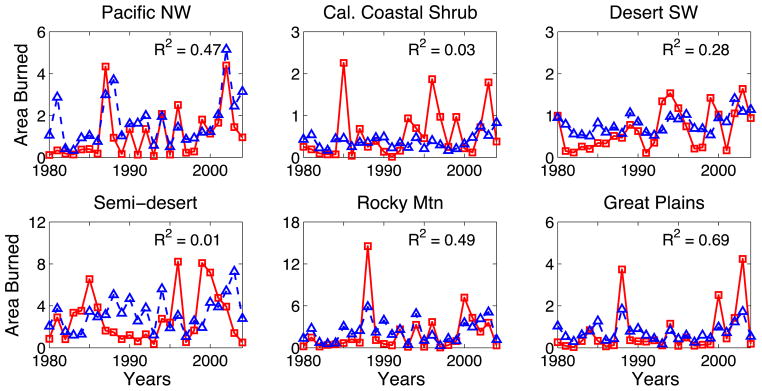
Time series of observed (red solid lines) and predicted (blue dashed lines) area burned (105 ha) for 1980–2004 using the parameterization. The NARR gridded reanalyses are used in simulation.
3. Ensemble projection of future area burned
We use both the regressions and parameterization with future climate from 15 GCMs to project future area burned in the mid 21st century. We assume that the relationships we derived between area burned and meteorological factors are the same in the future as at present. We use daily output from the NASA/GISS Model 3 (Hansen et al., 2002) and from 14 other GCMs in the CMIP3 archive (Meehl et al., 2007) (Table 2). The simulated meteorology includes daily mean and maximum temperature, total precipitation, and surface wind speed. We calculate daily RH for the CMIP3 models from other archived meteorological variables. Output from the Intergovernmental Panel on Climate Change (IPCC) 20C3M scenario is used for the present day (1981–2000). For this scenario, the models are freely running but forced by the well-mixed greenhouse gases increasing as observed in the 20th century. The resulting model meteorology matches the observed, but only in a decadal average sense. Output from the A1B scenario is used for the future (2046–2065). This scenario assumes significant innovations in energy technologies, which place more emphasis on non-fossil fuels, improve energy efficiency, and reduce the cost of energy supply, resulting in decreased CO2 emission after 2050. The 522 ppm of CO2 projected by 2050 in the A1B scenario is consistent with two moderate scenarios in the new Representative Concentration Pathways (RCPs) developed by the IPCC, RCP 6.0 and RCP 4.5 (Moss et al., 2010).
Table 2.
List of models a whose outputs are used in future fire projection.
| Model name | Resolution | Country |
|---|---|---|
| CCCMA-CGCM3.1 (T47) | 3.75°× 3.75° | Canada |
| CCCMA-CGCM3.1 (T63) | 2.8125°× 2.8125° | Canada |
| CNRM-CM3 | 2.8125° × 2.8125° | France |
| CSIRO-MK3.0 | 1.875° × 1.875° | Australia |
| CSIRO-MK3.5 | 1.875° × 1.875° | Australia |
| GFDL-CM2.0 | 2.5° × 2.0° | USA |
| GFDL-CM2.1 | 2.5° × 2.0° | USA |
| GISS-AOM | 4.0° × 3.0° | USA |
| IAP-FGOALS1.0 | 2.8125° × 3.0° | China |
| INGV-ECHAM4 | 1.125° × 1.125° | Italy |
| IPSL-CM4 | 3.75° × 2.5° | France |
| MIUB-ECHOG | 3.75° × 3.75° | Germany |
| MPI-ECHAM5 | 1.875° × 1.875° | Germany |
| MRI-CGCM2.3.2 | 2.8125° × 2.8125° | Japan |
| GISS-GCM3 | 5.0° × 4.0° | USA |
The meteorological fields for the first 14 models are from the CMIP3 archive (http://www-pcmdi.llnl.gov/). Other models in the archive did not provide required daily variables.
When applying the regressions to predict fires, we merge the monthly gridded output from each GCM into the six ecoregions and scale them using the mean observations for 1981–2000 from the USHCN. However, we scale the daily variables with the GSOD to calculate CFWIS indexes and monthly RH. The regressions predict some negative burned areas and we set these to zero. For the prediction with the parameterization, we interpolate the CMIP3 data with different spatial resolutions (Table 2) onto the same 1°×1° grid using the inverse distance weighted method, as in other studies (e.g. Balshi et al., 2009). The regridded daily GCM outputs are then scaled to the monthly mean NARR reanalyses of 1981–2000 for each grid box. Our approach does not resolve the impacts of topography on meteorology as well as the use of statistically downscaled GCM data might (Maurer et al., 2007), but CMIP3 downscaled datasets (e.g., http://gdo-dcp.ucllnl.org/) lack variables (RH and wind speed) needed for our prediction methods. The results given in this study for each ecoregion are shown as the median value of the ensemble of predictions from 15 GCMs and median value of the 15 ratios of predicted to observed area burned. We choose to use the median rather than the mean values to avoid skewing by extreme model results.
Prediction of present-day area burned with GCM meteorology reproduces observed values in most ecoregions for both regressions and the parameterization (Tables 3 and 4, and section E in the SI). In response to the warmer and drier summer climate (see section F in the SI), the median predicted area burned from the regressions increases in every ecoregion at the midcentury relative to present day, as shown in Table 3, and by Fig. 6a and Fig. 7a. The last column of Table 3 shows the number of models that predict a ratio within the range of ±20% of the median ratio, so higher numbers indicate greater agreement among the projections. The predicted time series for present-day area burned in Fig. 6a are much smoother than observed, as they show the median result of the 15 GCMs each year. The interannual variation is much greater for the individual models, and some of them predict a 30% higher standard deviation than do the observations. The regression method projects increases in annual area burned of 24–124% depending on ecoregion, with the largest median ratio of future to present-day area burned in the Desert Southwest (Fig. 7a). Table 3 and Fig. 7c show that only a few GCMs predict a significant increase in area burned for the Pacific Northwest and California Coastal Shrub, while most predict an increase in the desert and semi-desert regions. Ratios of future to present-day area burned for individual GCMs are shown in Fig. 7, and we discuss this figure below.
Table 3.
Observations and ensemble projections of area burned (104 ha) with regressions.
| Ecoregions | Observed a (1986–2000) | Present Day Regression b (1986–2000) | Future Regression b (2051–2065) | Ratio c (Future/Present) | # of models d (p<0.05) | # of models e (M±20%) |
|---|---|---|---|---|---|---|
| Pacific Northwest | 11.2 ± 12.0 | 11.3 ± 8.7 | 18.3 ± 10.2 | 1.42 | 5 | 10 |
| California Coastal Shrub | 5.4 ± 5.0 | 6.0 ± 3.2 | 7.0 ± 3.4 | 1.24 | 3 | 10 |
| Desert Southwest | 7.3 ± 4.7 | 6.5 ± 2.8 | 14.6 ± 3.2 | 2.24 | 15 | 13 |
| Nevada Mnts/Semi-desert | 28.1 ± 27.6 | 30.1 ± 18.5 | 48.9 ± 15.0 | 1.56 | 12 | 13 |
| Rocky Mnts Forest | 24.7 ± 38.6 | 35.9 ± 31.5 | 61.7 ± 33.0 | 1.71 | 8 | 6 |
| Eastern Rocky Mnts/Great Plains | 6.7 ± 10.6 | 6.9 ± 6.0 | 13.0 ± 6.5 | 1.62 | 9 | 5 |
| Western U.S. total | 83.3 ± 66.6 | 96.5 ± 50.9 | 155.3 ± 51.1 | 1.60 | 11 | 9 |
AB = area burned. Results in each ecoregion are shown as .
Result in each ecoregion are the median values of and σ predicted using the climate data from 15 GCMs for the A1B scenario.
Results in each ecoregion are the median value of 15 ratios of AB between midcentury (A1B) and present-day calculated with the GCM output.
Number out of 15 models who predict a significant (p<0.05) increase in AB in each ecoregion determined by a Student t-test.
Number out of 15 models who predict a ratio within the range of ±20% of the median ratio.
Table 4.
Observations and ensemble projections of area burned (104 ha) with the parameterization a.
| Ecoregions | Observed (1981–2000) | Present Day Param. (1981–2000) | Future Param. (2046–2065) | Ratio (Future/Present) | # of models (p<0.05) | # of models (M±20%) |
|---|---|---|---|---|---|---|
| Pacific Northwest | 9.1 ± 10.9 | 7.7 ± 5.0 | 19.8 ± 11.7 | 2.54 | 11 | 6 |
| Desert Southwest | 6.0 ± 4.7 | 6.2 ± 1.8 | 11.5 ± 3.3 | 1.63 | 15 | 12 |
| Rocky Mnts Forest | 20.2 ± 34.2 | 21.8 ± 15.8 | 98.8 ± 105.0 | 2.69 | 11 | 3 |
| Eastern Rocky Mnts/Great Plains | 5.8 ± 9.3 | 4.4 ± 2.1 | 14.0 ± 6.8 | 2.00 | 10 | 4 |
Results are shown with the same format as in Table 3, but for a different present-day time period.
Fig. 6.

Predicted annual mean area burned (105 ha) for the present day (1986–2000) and at midcentury (2051–2065) from 15 GCMs using (a) regressions and (b) the parameterization. The red lines are the observed area burned for the western U.S. (top panel) or for each ecoregion (lower panels) during 1986–2000. The blue lines are the yearly median values of the area burned predicted by the 15 GCMs. The gray shading shows the spread of the predictions.
Fig. 7.

Predicted ratio of future area burned to present day area burned over six ecoregions with (a) regressions and (b) parameterization. The short bold lines are the median ratios. The number of GCMs that predict significant (p < 0.05) increases in area burned is shown in (c) for regression and (d) for parameterization. The ecoregions are: PNW, Pacific Northwest; CCS, California Coastal Shrub; DSW, Desert Southwest; NMS, Nevada Mountains/Semi-desert; RMF, Rocky Mountains Forest; ERM, Eastern Rocky Mountains/Great Plains. Different symbols show results from different GCMs.
Table 5 shows the changes in regression terms and their contributions to the projected increases in area burned from the regressions. The Table makes clear the importance of considering variables other than just temperature when considering future fire activity. Changes in fuel moisture codes and temperature contribute the most to the change in area burned, and more GCMs predict significant changes in these factors than in relative humidity and rainfall. For the ecoregions where the changes in area burned are dominated by fuel moisture codes or temperature, we find that the GCMs that predict significant increases in those factors also predict significant increases in area burned (Tables 3 and 5). In two regions, the Pacific Northwest and California Coastal Shrub, the increases in area burned related to drought codes are offset to some extent by changes in relative humidity. Only a few GCMs predict significant increases in area burned in these regions (Table 3 and Fig. 7c).
Table 5.
Changes of meteorological variables and their contributions to the predicted changes in area burned calculated by regressions.
| Ecoregions | Simulated Median Mean
|
# of models (p<0.05) a | Changes in Reg. terms b | Percent Contribution c | |
|---|---|---|---|---|---|
| 1986–2000 | 2051–2065 | ||||
| Pacific Northwest | |||||
| BUI | 81.3 | 105.0 | 10 | 6.5 × 10⁴ | 64 |
| RH.ANN(-1) (%) | 69.2 | 68.8 | 4 | −3.8 × 10⁴ | 36 |
| California Coastal Shrub | |||||
| RH.WIN(-1) (%) | 68.5 | 67.8 | 2 | −2.2 × 10⁴ | 37 |
| DCmax | 1575.6 | 1654.4 | 10 | 3.7 × 10⁴ | 63 |
| Desert Southwest | |||||
| Tmax.ANN (°C) | 23.8 | 26.2 | 15 | 9.3 × 10⁴ | 89 |
| Tmax.WIN(-1) (°C) | 13.6 | 15.6 | 14 | −1.2 × 10⁴ | 11 |
| Nevada Mountains/Semi-desert | |||||
| RH.FS(-1) (%) | 41.5 | 39.7 | 6 | −1.5 × 10⁵ | 25 |
| Tmax.SUM (°C) | 29.1 | 31.7 | 15 | 4.0 × 10⁵ | 64 |
| Prec.SUM(-2) (mm day−1) | 0.62 | 0.57 | 4 | −0.7 × 10⁵ | 11 |
| Rocky Mountains Forest | |||||
| DMCmax | 238.9 | 298.7 | 8 | 2.7 × 10⁵ | 100 |
| Eastern Rocky Mtns/Great Plains | |||||
| DMCmax | 118.3 | 155.3 | 7 | 2.6 × 10⁴ | 59 |
| RH.ANN (%) | 54.6 | 53.9 | 5 | 1.8 × 10⁴ | 41 |
Number of models out of the 15 which predict significant (p<0.05) changes in meteorological variables in each ecoregion as determined by a Student t-test. If the median value of the change is positive, only those predicting a significant increase are counted and vice versa.
Results are calculated as the changes in variables multiplied by the regression coefficients for the median models. A median model is defined as a model that predicts median ratios of the area burned in a specific ecoregion as shown in Table 3.
Percent contributions of the absolute changes in individual regression terms to their sum for the median models.
The projections of future area burned with the parameterization are shown in Table 4 and Fig. 6b for the four ecosystems whose area burned is captured for the present-day using this approach. The parameterization yields increases of 63–169% in annual area burned, with the largest increases in the Pacific Northwest and the Rocky Mountain Forest (Table 4 and Fig. 7b). The parameterization method generally gives a higher ratio of future area burned to present day than does the regression approach, and the spread of area burned predicted by the 15 GCMs is generally larger (Figs. 6, 7) because of the exponential relationship.
Because temperature plays a major role in the parameterization, more GCMs predict significant increases in future area burned for forested ecoregions with this approach than with the regressions (Fig. 7d). As shown in Fig. S5, the projected median increases in summer temperature are greater than 2 °C in all ecoregions, and the decreases in relative humidity and precipitation are around 1% and 0.1 mm day−1, respectively. We explored the regional sensitivity of area burned to changes of this magnitude by first applying incremental changes to the NARR observed time series of temperature, relative humidity, and precipitation in each ecoregion and then recalculating area burned (Fig. 8). As expected, warmer temperatures and lower humidity and rainfall cause increases in area burned, and the responses to the first two are symmetric with respect to the sign of the change. The effect of the increase in rainfall is artificial, as it leads to daily rainfall and almost no burning. The results in Fig. 8 suggest that the changes in temperature are the primary driver of the increase in area burned, and that the two forested regions (Pacific Northwest and Rocky Mountains Forest) are most sensitive to increases in temperature.
Fig. 8.

Sensitivity of the parameterization to incremental changes in key meteorological variables. Values shown are the ratios of annual mean area burned calculated with perturbed variables to the area burned calculated with NARR meteorology, averaged over 1980–2004. Perturbations are to daily NARR temperature (± 1°C), relative humidity (± 1%), and precipitation (± 0.1 mm day−1). The ecoregions are: PNW, Pacific Northwest; CCS, California Coastal Shrub; DSW, Desert Southwest; NMS, Nevada Mountains/Semi-desert; RMF, Rocky Mountains Forest; ERM, Eastern Rocky Mountains/Great Plains.
Both the regression and the parameterization methods sometimes yield unrealistic projections of fire activity (Fig. 7). As noted above, predictions of negative area burned by the regressions are set to zero. Using the parameterization method, area burned increases by unreasonably large factors (10–70) with output from two GCMs in the Pacific Northwest, Rocky Mountain Forest, and Eastern Rocky Mountains/Great Plains. These same two models project large increases in temperature and large decreases in precipitation in summer for these regions, relative to other models (Fig. S5). Four other models give increases of factors of 6–15 for the Rocky Mountain Forest, again due to the relatively large changes in temperature and precipitation there. Except for these extreme cases, most models give ratios of 1–4 for future/present area burned in all ecoregions with either the regression or parameterization method. Predictions with the regressions show the largest uncertainty in the Eastern Rocky Mountains/Great Plains (Fig. 7a), because of the large spread of changes in meteorological variables that all contribute to increases in area burned (Fig. S5; Table 1). However, projections with the parameterization exhibit the largest uncertainty in the Rocky Mountains Forest (Fig. 7b), due to the large spread in the meteorological changes here as well and the high sensitivity of area burned to these changes.
An advantage of the parameterization method is that it predicts the seasonality of fires. Relative to present day, fires show larger area burned during the peak months. For example, area burned increases by 65% in August in the Pacific Northwest, 68% in June in Desert Southwest, 390% in August in Rocky Mountains Forest, and 190% in August in Eastern Rocky Mountains/Great Plains by the midcentury (Fig. 9). The probability of large fires, defined as the average percentage of grid cells that have daily area burned >100 ha during the fire season, is small for the present-day, 0.3% to ~2% for the four ecosystems, and increases by factors of 2 to 3 with the parameterization.
Fig. 9.
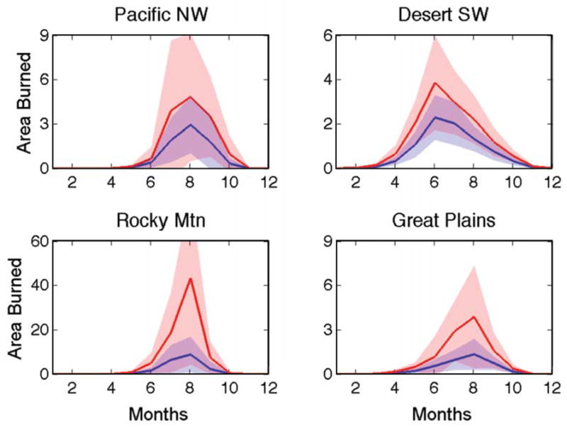
Predicted median area burned (104 ha) each month for the present day (1981–2000, blue lines) and at midcentury (2046–2065, red lines) with meteorological variables from 15 GCMs, using the parameterization. The pink and purple shadings show the median standard deviation.
We examine the predicted length of fire season, which we define as the period when the daily area burned is larger than 100 ha in at least one grid box (1°×1°). In response to the changing climate, the median start date changes from May 12 to April 28 and the median end date from October 4 to October 14, so that the median length of the fire season increases by over 3 weeks or 16% (Fig. 10). This change is robust, with 14 out of 15 GCMs projecting significant increases in length (p < 0.05). In most models, the fire season begins in the Desert Southwest and ends in the Pacific Northwest in both the present-day and future atmospheres. The median length of the period with large fires (>100 ha) increases by 20–42% in the four ecoregions, with the largest extension in the Eastern Rocky Mountains/Great Plains. Our results are consistent with the extension of fire season in boreal and temperate areas as projected by previous studies (Wotton and Flannigan, 1993).
Fig. 10.

Predicted length of fire season for the present day (1981–2000) and midcentury (2046–2065) over western United States with 15 climate models. The fire season is defined as the period when the daily area burned is larger than 100 ha in at least one grid box (1°×1°) over the four ecoregions in Fig. 9. The red lines are simulated results with NARR dataset for the present-day. The blue lines show the median length of fire season predicted with the 15 GCMs. The gray shading shows the spread of the predictions. Relative to the present-day medians, fire season lengthens by 23 days on average at the midcentury.
4. Estimate of future biomass burned
Fuel consumption is the amount of both live and dead biomass burned per unit area. We calculate present-day fuel consumption based on the fuel load database of the United States Forest Service, the Fuel Characteristic Classification System (http://www-fs-fed-us/pnw/fera/fccs/-downloaded-on-Ma-2011 FCCS, http://www.fs.fed.us/pnw/fera/fccs/, downloaded on May 12th, 2011) (McKenzie et al., 2007; Ottmar et al., 2007). The 1 km × 1 km fuelbed map for the conterminous U.S. is derived from the distribution of vegetation types from the Landscape Fire and Resource Management Planning Tools (LANDFIRE, http://www.landfire.gov/). This is a more complete version of the FCCS than available at the time of the S2009 study. We calculate fuel consumption following Table 4 of S2009. As in S2009, we assume that fires burn with 25% high, 25% medium, and 25% low severity, with 25% of the area unburned. An updated map of fuel consumption is shown in Fig. 11a. The value ranges from 0–1 kg dry mass (DM) m−2 in arid and semi-arid southwestern area. However, in northern forest region, the fuel consumption is as high as 9.5 kg DM m−2. We acknowledge that using the fixed fuel consumption map does not reflect the impact of interannual variability of biomass on fire emissions. We assume that fuel consumption throughout the western U.S. remains constant for 50-year period, because the simulation with a DGVM shows small changes in the cover of vegetation with a high fuel load (see section G in the SI).
Fig. 11.

(a) Fuel consumption calculated from the Fuel Characteristic Classification System database. (b) Mean annual biomass burned during 1980–2004 based on observed area burned. Projected annual biomass burned for the present day (c, d) and midcentury (e, f) with regressions (c, e) or the parameterization (d, f). Results for regressions are during 1986–2000 for the present day and 2051–2065 for mid-century. For parameterization, the two periods are 1981–2000 and 2046–2065. We show different time periods for the two approaches since the regression model requires two years of antecedent meteorology.
The annual mean biomass burned (Fig. 11b and Table 6) is the product of gridded area burned and fuel consumption. The largest values of present-day biomass burned are located in forest ecoregions, with 30% in the Pacific Northwest and 39% in the Rocky Mountains Forest. Although the Nevada Mountains/Semi-desert ecoregion has the largest area burned (35% of the total), it contributes only 9% to the total biomass burned because of low fuel availability (Table 6). The annual total biomass burned by wildfire is 13.0 Tg during 1980–2004 over the western United States. This is smaller than the estimate in S2009, 14.2 Tg, because of the updated FCCS fuel bed map.
Table 6.
Annual mean dry biomass consumption from wildfire over western U.S.
| Ecoregions | Annual Mean Biomass Consumption (Tg)
|
||||
|---|---|---|---|---|---|
| Observed (1980–2004) | Regression a | Parameterization a | |||
|
| |||||
| 1986–2000 | 2051–2065 | 1981–2000 | 2046–2065 | ||
| Pacific Northwest | 3.94 | 4.72 | 8.48 | 3.21 | 6.15 |
| California Costal Shrub | 0.64 | 0.75 | 0.87 | N/A | N/A |
| Desert Southwest | 0.34 | 0.25 | 0.55 | 0.25 | 0.44 |
| Nevada Mountains/Semi-desert | 1.22 | 1.72 | 2.47 | N/A | N/A |
| Rocky Mountains Forest | 5.05 | 8.63 | 15.6 | 5.09 | 18.0 |
| Eastern Rocky Mountains/Great Plans | 1.78 | 0.89 | 2.16 | 0.66 | 1.66 |
| Western U.S. Total | 13.0 | 17.0 | 30.1 | 12.1 b | 29.1 b |
The years for regression and parameterization are different because the projected area burned with two methods have different time spans.
Present-day (1981–2000) and midcentury (2046–2065) biomass burned over California Costal Shrub and Nevada Mountains/Semi-desert are calculated by using the observed monthly area burned from 1999–2004 in these two ecoregions.
To obtain the GCM estimates of biomass burned, we combine the projected area burned that has been allocated to the 1°×1° grid (see section H of the SI) with the fuel consumption. As shown in Fig. 11c, the present-day biomass burned calculated with the median area burned predicted by the regressions resembles that based on the observed area burned (Fig. 11b). The prediction overestimates biomass burned in the Rocky Mountains Forest (especially in Montana) by as much as 70%. The predicted total biomass burned over the western United States for the regression method is 17.0 Tg yr−1 for 1986–2000 (Table 6), higher than the value based on observed area burned, 13.0 Tg yr−1. The parameterization predicts slightly smaller present-day biomass burned (Fig. 11d), 12.1 Tg yr−1. These differences reflect the discrepancies between modeled and observed area burned for the two methods (Tables 3 and 4).
The median values of future area burned predicted by the two approaches are used to calculate future biomass burned as shown in Figs. 11e and 11f and Table 6. Both methods predict similar spatial patterns and larger amounts of biomass burned at midcentury, with the greatest increases in the Pacific Northwest and the Rocky Mountain Forest. The annual total biomass burned over the western United States increases by 77% with the regressions and 140% with parameterization.
5. Simulations of carbonaceous aerosols
We calculate the future fire emission based on the predicted biomass burned and the emission factors from Andreae and Merlet (2001). With the median area burned predicted by the regressions, we estimate that the total wildfire emission is 133 Gg C yr−1 for OC and 9 Gg C yr−1 for BC over the western United States for the present day, somewhat larger than the values calculated with observed area burned, 95 Gg C yr−1 for OC and 7 Gg C yr−1 for BC, due to the overestimate of present-day area burned in Rocky Mountains Forest by regressions (Table 3). The predicted emissions increase by ~80 % for both OC (to 238 Gg C yr−1) and BC (to 16 Gg C yr−1) by midcentury. Results from the parameterization give present-day emissions of 88 Gg C yr−1 for OC and 6 Gg C yr−1 for BC. These emissions increase by ~170 % for OC (to 235 Gg C yr−1) and ~150 % for BC (to 16 Gg C yr−1) by the midcentury.
To simulate the distributions of BC and OC over the western United States in the present-day and future atmospheres, we use the GEOS-Chem CTM (v08.03.01). The CTM, driven with present-day and future meteorological fields from the GISS GCM3, has been used to estimate the impact of changing climate on the future air quality in the United States (e.g., Wu et al., 2008; S2009). The model set-up is similar to that described in S2009, and we note any differences below.
The CTM transports hydrophobic and hydrophilic BC and OC. Hydrophobic aerosols become hydrophilic with an e-folding time of 1.2 days (Cooke et al., 1999). Global anthropogenic and biofuel emissions for BC and OC are from Bond et al. (2007); the emissions over North America are imposed with the seasonality following Park et al. (2003). Outside the western United States, climatological biomass burning emissions are from Lobert et al. (1999), with seasonality from Duncan et al. (2003). The main biogenic sources for OC are terpenes, which are calculated with the Model of Emissions of Gases and Aerosols from Nature (MEGAN), version 2.1 (Guenther et al., 2006). We assume a 10% yield of hydrophilic OC from these emissions. To isolate the effects of changes in fires in this study, we use constant emissions from anthropogenic and biofuel emissions and from biomass burning outside the western United States. Biogenic emissions vary in response to the changing climate.
We conduct three simulations for the present day (1997–2001) and for midcentury (2047–2051), with a six month spin-up, as shown in Table 7. These include simulations with monthly fire emissions from the median of GCMs predictions with the regression (Reg) and the parameterization (Param), and one with daily emissions from the latter (Param.D). We first aggregate the 1°×1° calculated fire emissions onto the 4°×5° grids of the CTM. Since our use of median values smoothes the interannual variability of area burned, we use the same total amount of area burned in a specific month in a given simulation each year, but the locations of fires are redistributed every year with the random method described in H of the SI.
Table 7.
List of numerical simulations with the GEOS-Chem CTMa
| Simulations | Period | Fire emissions
|
|
|---|---|---|---|
| Fire Model | Time scaleb | ||
| PD.Reg | 1997–2001 | Regression | Monthly |
| PD.Param | 1997–2001 | Parameterization | Monthly |
| PD.Param.D | 1997–2001 | Parameterization | Daily |
| A1B.Reg | 2047–2051 | Regression | Monthly |
| A1B.Param | 2047–2051 | Parameterization | Monthly |
| A1B.Param.D | 2047–2051 | Parameterization | Daily |
All the simulations are carried out with the CTM driven by meteorological data archived from the GISS GCM3
This is the temporal resolution of fire emissions (either monthly or daily) used in the simulations.
We first examine our present-day simulations of carbonaceous aerosol using the median wildfire emissions from the 15 GCMs. With the regression method, the CTM simulates highest concentrations for OC, ~2.0 μg m−3, in Oregon, Idaho, and western Montana during summer in the present (Fig. 12a). The BC concentrations are relatively high, ~0.2 μg m−3, in these regions as well (Fig. 12c), but high values are also predicted over the coastal states without large fire emissions, because the dominant fraction (>70%) of BC emission is from fossil fuel combustion (Park et al., 2003). The CTM driven by fire emissions from the parameterization gives similar present-day distributions of OC (Fig. 12b) and BC (Fig. 12d) compared with those from the regressions, but with smaller magnitudes due to the smaller fire emissions.
Fig. 12.

Simulated June-August surface concentrations of (left 2 columns) OC and (right 2 columns) BC aerosol over the western United States during (a, b, c, d) 1997–2001 and (e, f, g, h) 2047–2051. Results are from the GEOS-Chem CTM using the median predicted fire emissions from the 15 GCMs with (1st and 3rd columns) regressions and (2nd and 4th columns) the parameterization. The bottom panel shows the change in simulated concentrations between the two time periods.
At mid-century using both approaches, the simulated OC and BC fields show large increases in summer, relative to the present-day. With the regression method, the mean summertime concentration of OC aerosol increases from 0.96 μg m−3 in the present-day to 1.40 μg m−3 in the future (46%), while mean BC increases from 0.14 to 0.17 μg m−3 (20%). The increase is most prominent over Oregon, Idaho, western Montana, and Wyoming (1.15 μg m−3 for OC and 0.07 μg m−3 for BC, Figs. 12i and k). Similar results are obtained in the simulation using the parameterization method (Figs. 12j and l), which predicts a 70% increase of mean OC aerosol from 0.89 μg m−3 in the present-day to 1.41 μg m−3. BC for this method increases 27%, from 0.13 μg m−3 to 0.17 μg m−3. We calculate the greatest change in Idaho, where OC increases by 1.59 μg m−3 and BC by 0.09 μg m−3. In the simulations for mid-century, biogenic OC emissions increase by 30 Gg C yr−1 (19%), due to higher temperatures. However, this increase is much smaller than the increase in fire emissions from the regression and parameterization approaches, 105 Gg C yr−1 and 148 Gg C yr−1 respectively. More than 77% of the changes in OC may be attributed to the changes in wildfire emissions, similar to the estimate by S2009.
Using the simulations with the parameterization of area burned, we examine the impact of climate change on the frequency of extreme pollution events from wildfires in 32 Federal Class 1 areas (http://www.epa.gov/) in the Rocky Mountains Forest ecoregion as shown in Fig. 13. Values at the high end of the distributions represent pollution episodes. We find that future wildfire activity would increase aerosol levels dramatically on pollution days. For days characterized by aerosol levels above the 84th percentile (i.e., the most polluted 30 days during the fire season), OC increases on average by ~90% (1.55 μg m−3) and BC increases by ~50% (0.09 μg m−3). Following the method in Park et al. (2006) we estimate that such enhancement in air pollutants increases the average haze index from 10.9 deciviews to 13.5 deciviews (> 84th percentile, Fig. 13c), which corresponds to a change in visibility from 130 km to 100 km based on the definition in Pitchford and Malm (1994). Our predictions are conservative since we use daily emissions based on the median area burned.
Fig. 13.

Cumulative probability distributions of daily mean (a) OC concentrations, (b) BC concentrations, and (c) haze index in deciviews in 32 Federal Class 1 areas in the Rocky Mountains Forest ecoregion in 2000 (blue points) and 2050 (red points). Each point represents average aerosol concentrations or haze index in one area on one day of the fire season (May-October). Emissions are calculated from the predictions using the parameterization.
6. Discussion and Conclusions
We estimated the changes in future wildfire activity and their impact on carbonaceous aerosols over the western United States during the mid-21st century (2046–2065). We developed both regressions and a parameterization as fire prediction tools and used an ensemble of climate model projections for 2050 conditions together with the CTM GEOS-Chem. Use of this ensemble allowed us to predict trends in future fire activity with greater confidence than previous studies, and to diagnose the consequences of these trends for air quality across the western United States. We list the key results for our study below, followed by a more detailed summary of our results.
The median model results show consistent increases of 24–169% in area burned across much of the western United States in the warmer and drier future atmosphere, regardless of projection method.
For the regressions, most GCMs show significant increases in area burned in the Desert Southwest, Nevada Mountains/Semi-desert, Rocky Mountains Forest, and Eastern Rocky Mountains/Great Plains. The projections are less robust in the Pacific Northwest and California Coastal Shrub ecoregions.
For the parameterization, most GCMs predict significant increases in area burned in the Pacific Northwest, Desert Southwest, Rocky Mountains Forest, and Eastern Rocky Mountains/Great Plains.
Both regressions and the parameterization best capture the observed interannual variability of wildfires over forested regions. In addition, the parameterization successfully represents the seasonality of area burned in most regions of western United States. In response to the warmer and drier summer climate in the A1B scenario, the regressions project that the annual area burned will increase by 24–124%, with the largest increases in the Desert Southwest where the area burned is especially sensitive to temperature. Under the same climate scenario, the parameterization projects increases of 63–169% in annual area burned, but with the largest relative increases in the Pacific Northwest and the Rocky Mountain Forest. Using the parameterization, we showed that the length of the fire season increases by more than three weeks in the future atmosphere. These changes in fire emissions worsen air quality by the midcentury. Using the area burned from regressions, GEOS-Chem simulations predict that the summertime mean surface aerosol concentrations will increase by 46% for OC and 20% for BC during 2047–2051 relative to the values in 1997–2001. With the parameterization, these changes are 70% and 27% respectively. The intensified wildfire activity has a larger impact on the extreme events.
To our knowledge, this is the first time an ensemble of climate models has been applied to present-day relationships between meteorology and area burned to calculate the effect of changing climate on the area burned by wildfires and the resultant pollution. Our use of an ensemble provides confidence in our main results, that fire activity will increase in the future atmosphere, with potentially serious consequences for air quality. Although the climate models show large variation in their projections of key variables associated with fire weather, application of a multi-model approach allows us to overcome the challenges posed by these variations by focusing on median results and the number of GCMs that give significant changes in area burned.
Our use of a multi-model ensemble allowed us not only to identify robust results, but also to quantify the uncertainty in our projections and to diagnose model outliers. While all models project significant increases in surface temperature averaged over the West, the spread in model response is several degrees. Trends in precipitation and relative humidity, on the other hand, are not robust across models for the region. The western U.S. lies in a transition zone between the low latitudes, where most models project drier conditions in a future atmosphere, and higher latitudes, where most models predict a more moist climate (Christensen et al., 2007). These differences among climate models in the projections of future temperature, precipitation, and relative humidity lead to substantial variation among the projections for area burned, particularly for the parameterization approach. By examining the median response in fire activity to changing climate conditions, we discounted the results from outlier models in our study.
Wildfire is a consequence of the interactions between climate, people, and fuels. In this study we focus only on the impact of climate change alone because this factor has the dominant impact on the size, timing and severity of fires (Bessie and Johnson, 1995). However, other factors could also influence future wildfires. For example, decades of effective fire suppression in the West has promoted the unnatural accumulation of forest fuels and may increase the probability of unprecedentedly large fires in the future (Schoennagel et al., 2004), an effect we do not take into account.
Given this limitation, our study shows that wildfire activity will likely increase in the western U.S. in the warmer A1B climate at mid-century. Our regression approach shows area burned doubling in the Desert Southwest by 2050, while our parameterization predicts area burned doubling across the Pacific Northwest, Rocky Mountains Forest, and the Eastern Rockies/Great Plains. These increases in area burned together with the longer fire season calculated in our study could significantly limit visibility in parks and wilderness areas and worsen regional air quality.
Supplementary Material
Table S1 Studies projecting future area burned in North America
Table S2 Simulated changes in the vegetation cover fraction by LPJ DGVM
Table S3 Area and area burned fraction of each Bailey ecosystem a to the corresponding aggregated ecoregion b during 1980–2004.
Fig. S1. Log10 of annual mean (a) observed and (b) simulated area burned (ha) averaged from 1980 to 2004. The simulated result is from the parameterization.
Fig. S2. Seasonality of simulated (blue dashed lines) and observed (red solid lines) area burned (104 ha) in each ecoregion. Simulations are from the parameterization. Each point represents the monthly mean for 1980–2004.
Fig. S3. (a) Ratios of predicted to observed present-day area burned. The simulated results are from the regressions. (b) Same as (a) but for results from the parameterization. The ecoregions are: PNW, Pacific Northwest; CCS, California Coastal Shrub; DSW, Desert Southwest; NMS, Nevada Mountains/Semi-desert; RMF, Rocky Mountains Forest; ERM, Eastern Rocky Mountains/Great Plains. Different symbols are used for each model. The short bold lines are the median ratios. No results are shown for the California Coastal Shrub and Nevada Mountains/Semi-desert regions in (b) because the parameterization does not reproduce the interannual variations of area burned there.
Fig. S4. Median changes in seasonal mean meteorological fields from 15 climate models following the A1B scenario for 2046–2065, relative to present-day (20C3M, 1981–2000) over western U.S. The left panels are for winter, the right panels for summer, with temperature, precipitation and relative humidity from top to bottom.
Fig. S5. Projected changes in (a) temperature, (b) precipitation, and (c) relative humidity for six ecoregions in summer by midcentury for 15 climate models. The ecoregions are: PNW, Pacific Northwest; CCS, California Coastal Shrub; DSW, Desert Southwest; NMS, Nevada Mountains/Semi-desert; RMF, Rocky Mountains Forest; ERM, Eastern Rocky Mountains/Great Plains. Different symbols are used for each model. The short bold lines are the median values.
Highlights.
We apply ensemble projection for future wildfire using output from 15 GCMs
We develop and evaluate both regressions and a parameterization for fire predictions
We investigate the impacts of climate change on fuel load by the midcentury
We examine fire-induced changes in OC/BC by the midcentury
is the long-term average of the AB during fire season (May-October), σ is the corresponding standard deviation.
Acknowledgments
We thank Eric M. Leibensperger for his help in handling the GSOD data. We acknowledge the modeling groups, the Program for Climate Model Diagnosis and Intercomparison (PCMDI) and the WCRP’s Working Group on Coupled Modelling (WGCM) for their roles in making available the WCRP CMIP3 multi-model dataset. Support of this dataset is provided by the Office of Science, U.S. Department of Energy. This work was funded by STAR Research Assistance agreement R834282 awarded by the U.S. Environmental Protection Agency (EPA). Although the research described in this article has been funded wholly or in part by the EPA, it has not been subjected to the Agency’s required peer and policy review and therefore does not necessarily reflect the views of the Agency and no official endorsement should be inferred. Research reported in this publication was supported in part by the National Institutes of Health (NIH) under Award Numbers 1R21ES021427 and 5R21ES020194. The content is solely the responsibility of the authors and does not necessarily represent the official views of the NIH.
Footnotes
Publisher's Disclaimer: This is a PDF file of an unedited manuscript that has been accepted for publication. As a service to our customers we are providing this early version of the manuscript. The manuscript will undergo copyediting, typesetting, and review of the resulting proof before it is published in its final citable form. Please note that during the production process errors may be discovered which could affect the content, and all legal disclaimers that apply to the journal pertain.
References
- Andreae MO, Merlet P. Emission of trace gases and aerosols from biomass burning. Global Biogeochemical Cycles. 2001;15:955–966. [Google Scholar]
- Bailey R, Avers P, King T, McNab W. Ecoregions and subregions of the United States (map) USDA For. Serv; Washington, D. C: 1994. [Google Scholar]
- Balshi MS, McGuirez AD, Duffy P, Flannigan M, Walsh J, Melillo J. Assessing the response of area burned to changing climate in western boreal North America using a Multivariate Adaptive Regression Splines (MARS) approach. Global Change Biology. 2009;15:578–600. doi: 10.1111/J.1365-2486.2008.01679.X. [DOI] [Google Scholar]
- Bessie WC, Johnson EA. The relative importance of fuels and weather on fire behavior in subalpine forests. Ecology. 1995;76:747–762. [Google Scholar]
- Bond TC, Bhardwaj E, Dong R, Jogani R, Jung S, Roden C, Streets DG, Trautmann NM. Historical emissions of black and organic carbon aerosol from energy-related combustion. Global Biogeochemical Cycles. 2007;21:GB2018. doi: 10.1029/2006GB002840. [DOI] [Google Scholar]
- Christensen JH, Hewitson B, Busuioc A, Chen A, Gao X, Held I, Jones R, Kolli RK, Kwon W-T, Laprise R, Rueda VMa, Mearns L, Menéndez CG, Räisänen J, Rinke A, Sarr A, Whetton P. Regional Climate Projections. In: Solomon S, Qin D, Manning M, Chen Z, Marquis M, Averyt KB, Tignor M, Miller HL, editors. Climate Change 2007: Working Group I: The Physical Science Basis. Cambridge University Press; Cambridge, United Kingdom and New York, NY, USA: 2007. [Google Scholar]
- Cooke WF, Liousse C, Cachier H, Feichter J. Construction of a 1° × 1° fossil fuel emission data set for carbonaceous aerosol and implementation and radiative impact in the ECHAM4 model. Journal of Geophysical Research. 1999;104:22137–22162. [Google Scholar]
- Crevoisier C, Shevliakova E, Gloor M, Wirth C, Pacala S. Drivers of fire in the boreal forests: Data constrained design of a prognostic model of burned area for use in dynamic global vegetation models. Journal of Geophysical Research. 2007;112:D24112. doi: 10.1029/2006jd008372. [DOI] [Google Scholar]
- Crimmins MA, Comrie AC. Interactions between antecedent climate and wildfire variability across south-eastern Arizona. International Journal of Wildland Fire. 2004;13:455–466. doi: 10.1071/Wf03064. [DOI] [Google Scholar]
- Duncan BN, Martin RV, Staudt AC, Yevich R, Logan JA. Interannual and seasonal variability of biomass burning emissions constrained by satellite observations. Journal of Geophysical Research. 2003;108:4100. doi: 10.1029/2002jd002378. [DOI] [Google Scholar]
- Easterling DR, Karl TR, Mason EH, Hughes PY, Bowman DP. United States Historical Climatology Network (US HCN) Monthly Temperature and Precipitation Data, ORNL/CDIAC-87, NDP-019/R3. Carbon Dioxide Information Analysis Center, Oak Ridge National Laboratory, U.S. Department of Energy; Oak Ridge, Tennessee: 1996. [Google Scholar]
- Flannigan MD, Harrington JB. A Study of the Relation of Meteorological Variables to Monthly Provincial Area Burned by Wildfire in Canada (1953–80) Journal of Applied Meteorology. 1988;27:441–452. [Google Scholar]
- Flannigan MD, Logan KA, Amiro BD, Skinner WR, Stocks BJ. Future area burned in Canada. Climatic Change. 2005;72:1–16. doi: 10.1007/S10584-005-5935-Y. [DOI] [Google Scholar]
- Flannigan MD, Krawchuk MA, de Groot WJ, Wotton BM, Gowman LM. Implications of changing climate for global wildland fire. International Journal of Wildland Fire. 2009;18:483–507. doi: 10.1071/Wf08187. [DOI] [Google Scholar]
- Gillett NP, Weaver AJ, Zwiers FW, Flannigan MD. Detecting the effect of climate change on Canadian forest fires. Geophysical Research Letter. 2004;31:L18211. doi: 10.1029/2004gl020876. [DOI] [Google Scholar]
- Guenther A, Karl T, Harley P, Wiedinmyer C, Palmer PI, Geron C. Estimates of global terrestrial isoprene emissions using MEGAN (Model of Emissions of Gases and Aerosols from Nature) Atmospheric Chemistry and Physics. 2006;6:3181–3210. [Google Scholar]
- Hansen J, Sato M, Nazarenko L, Ruedy R, Lacis A, Koch D, Tegen I, Hall T, Shindell D, Santer B, Stone P, Novakov T, Thomason L, Wang R, Wang Y, Jacob D, Hollandsworth S, Bishop L, Logan J, Thompson A, Stolarski R, Lean J, Willson R, Levitus S, Antonov J, Rayner N, Parker D, Christy J. Climate forcing in Goddard Institure for Space Studies SI2000 simulations. Journal of Geophysical Research. 2002;107:4347. doi: 10.1029/2001JD001143. [DOI] [Google Scholar]
- Littell JS, McKenzie D, Peterson DL, Westerling AL. Climate and wildfire area burned in western U. S. ecoprovinces, 1916–2003. Ecological Applications. 2009;19:1003–1021. doi: 10.1890/07-1183.1. [DOI] [PubMed] [Google Scholar]
- Lobert JM, Keene WC, Logan JA, Yevich R. Global chlorine emissions from biomass burning: Reactive Chlorine Emissions Inventory. Journal of Geophysical Research. 1999;104:8373–8389. [Google Scholar]
- Maurer EP, Brekke L, Pruitt T, Duffy PB. Fine-resolution climate projections enhance regional climate change impact studies. EOS Trans AGU. 2007;88 doi: 10.1029/2007EO470006. [DOI] [Google Scholar]
- McKenzie D, Raymond CL, Kellogg LKB, Norheim RA, Andreu AG, Bayard AC, Kopper KE, Elman E. Mapping fuels at multiple scales: landscape application of the Fuel Characteristic Classification System. Canadian Journal of Forest Research. 2007;37:2421–2437. doi: 10.1139/X07-056. [DOI] [Google Scholar]
- Meehl GA, Covey C, Delworth T, Latif M, McAvaney B, Mitchell JFB, Stouffer RJ, Taylor KE. The WCRP CMIP3 multi-model dataset: A new era in climate change research. Bulletin of the American Meteorological Society. 2007;88:1383–1394. doi: 10.1175/BAMS-88-9-1383. [DOI] [Google Scholar]
- Mesinger F, DiMego G, Kalnay E, Mitchell K, Shafran PC, Ebisuzaki W, Jovic D, Woollen J, Rogers E, Berbery EH, Ek MB, Fan Y, Grumbine R, Higgins W, Li H, Lin Y, Manikin G, Parrish D, Shi W. North American regional reanalysis. Bulletin of the American Meteorological Society. 2006;87:343–360. doi: 10.1175/Bams-87-3-343. [DOI] [Google Scholar]
- Moss RH, Edmonds JA, Hibbard KA, Manning MR, Rose SK, van Vuuren DP, Carter TR, Emori S, Kainuma M, Kram T, Meehl GA, Mitchell JFB, Nakicenovic N, Riahi K, Smith SJ, Stouffer RJ, Thomson AM, Weyant JP, Wilbanks TJ. The next generation of scenarios for climate change research and assessment. Nature. 2010;463:747–756. doi: 10.1038/Nature08823. [DOI] [PubMed] [Google Scholar]
- Ottmar RD, Sandberg DV, Riccardi CL, Prichard SJ. An overview of the Fuel Characteristic Classification System - Quantifying, classifying, and creating fuelbeds for resource planning. Canadian Journal of Forest Research. 2007;37:2383–2393. doi: 10.1139/X07-077. [DOI] [Google Scholar]
- Park RJ, Jacob DJ, Chin M, Martin RV. Sources of carbonaceous aerosols over the United States and implications for natural visibility. Journal of Geophysical Research. 2003;108:4355. doi: 10.1029/2002JD003190. [DOI] [Google Scholar]
- Park RJ, Jacob DJ, Kumar N, Yantosca RM. Regional visibility statistics in the United States: Natural and transboundary pollution influences, and implications for the Regional Haze Rule. Atmospheric Environment. 2006;40:28. doi: 10.1016/J.Atmosenv.2006.04.059. [DOI] [Google Scholar]
- Pechony O, Shindell DT. Fire parameterization on a global scale. Journal of Geophysical Research. 2009;114:D16115. doi: 10.1029/2009jd011927. [DOI] [Google Scholar]
- Philippi TE. Multiple regression: Herbivory. In: Scheiner S, Gurevitch J, editors. Design and Analysis of Ecological Experiments. Chapman & Hall; New York: 1993. [Google Scholar]
- Pitchford ML, Malm WC. Development and Applications of a Standard Visual Index. Atmospheric Environment. 1994;28:1049–1054. doi: 10.1016/1352-2310(94)90264-X. [DOI] [Google Scholar]
- Prichard SJ, Peterson DL, Jacobson K. Fuel treatments reduce the severity of wildfire effects in dry mixed conifer forest, Washington, USA. Canadian Journal of Forest Research. 2010;40:1615–1626. doi: 10.1139/X10-109. [DOI] [Google Scholar]
- Schoennagel T, Veblen TT, Romme WH. The interaction of fire, fuels, and climate across Rocky Mountain forests. BioScience. 2004;54:661–676. [Google Scholar]
- Spracklen DV, Mickley LJ, Logan JA, Hudman RC, Yevich R, Flannigan MD, Westerling AL. Impacts of climate change from 2000 to 2050 on wildfire activity and carbonaceous aerosol concentrations in the western United States. Journal of Geophysical Research. 2009;114:D20301. doi: 10.1029/2008jd010966. [DOI] [Google Scholar]
- Thonicke K, Spessa A, Prentice IC, Harrison SP, Dong L, Carmona-Moreno C. The influence of vegetation, fire spread and fire behaviour on biomass burning and trace gas emissions: results from a process-based model. Biogeosciences. 2010;7:1991–2011. doi: 10.5194/Bg-7-1991-2010. [DOI] [Google Scholar]
- Val Martin M, Honrath RE, Owen RC, Pfister G, Fialho P, Barata F. Significant enhancements of nitrogen oxides, black carbon, and ozone in the North Atlantic lower free troposphere resulting from North American boreal wildfires. Journal of Geophysical Research. 2006;111:D23s60. doi: 10.1029/2006jd007530. [DOI] [Google Scholar]
- Van Wagner CE. Forest Technical Report. Vol. 35. Canadian Forest Service; Ottawa, Canada: 1987. The development and structure of the Canadian forest fire weather index system. [Google Scholar]
- Westerling AL, Gershunov A, Cayan DR, Barnett TP. Long lead statistical forecasts of area burned in western US wildfires by ecosystem province. International Journal of Wildland Fire. 2002;11:257–266. doi: 10.1071/Wf02009. [DOI] [Google Scholar]
- Westerling AL, Hidalgo HG, Cayan DR, Swetnam TW. Warming and earlier spring increase western US forest wildfire activity. Science. 2006;313:940–943. doi: 10.1126/Science.1128834. [DOI] [PubMed] [Google Scholar]
- Wotawa G, Trainer M. The influence of Canadian forest fires on pollutant concentrations in the United States. Science. 2000;288:324–328. doi: 10.1126/science.288.5464.324. [DOI] [PubMed] [Google Scholar]
- Wotton BM, Flannigan MD. Length of the Fire Season in a Changing Climate. Forestry Chronicle. 1993;69:187–192. [Google Scholar]
- Wu S, Mickley LJ, Jacob DJ, Rind D, Streets DG. Effects of 2000–2050 changes in climate and emissions on global tropospheric ozone and the policy-relevant background surface ozone in the United States. Journal of Geophysical Research. 2008;113:D18312. doi: 10.1029/2007JD009639. [DOI] [Google Scholar]
References
- Amiro BD, Cantin A, Flannigan MD, de Groot WJ. Future emissions from Canadian boreal forest fires. Canadian Journal of Forest Research. 2009;39:383–395. doi: 10.1139/X08-154. [DOI] [Google Scholar]
- Arora VK, Boer GJ. Fire as an interactive component of dynamic vegetation models. J Geophys Res. 2005;110:G02008. doi: 10.1029/2005jg000042. [DOI] [Google Scholar]
- Bachelet D, Neilson RP, Lenihan JM, Drapek RJ. Climate change effects on vegetation distribution and carbon budget in the United States. Ecosystems. 2001;4:164–185. [Google Scholar]
- Bachelet D, Neilson RP, Hickler T, Drapek RJ, Lenihan JM, Sykes MT, Smith B, Sitch S, Thonicke K. Simulating past and future dynamics of natural ecosystems in the United States. Global Biogeochemical Cycles. 2003;17 doi: 10.1029/2001gb001508. [DOI] [Google Scholar]
- Bachelet D, Lenihan J, Neilson R, Drapek R, Kittel T. Simulating the response of natural ecosystems and their fire regimes to climatic variability in Alaska. Canadian Journal of Forest Research. 2005;35:2244–2257. doi: 10.1139/X05-086. [DOI] [Google Scholar]
- Balshi MS, McGuirez AD, Duffy P, Flannigan M, Walsh J, Melillo J. Assessing the response of area burned to changing climate in western boreal North America using a Multivariate Adaptive Regression Splines (MARS) approach. Global Change Biology. 2009;15:578–600. doi: 10.1111/J.1365-2486.2008.01679.X. [DOI] [Google Scholar]
- Cardoso MF, Hurtt GC, Moore B, Nobre CA, Prins EM. Projecting future fire activity in Amazonia. Global Change Biology. 2003;9:656–669. doi: 10.1046/j.1365-2486.2003.00607.x. [DOI] [Google Scholar]
- Crevoisier C, Shevliakova E, Gloor M, Wirth C, Pacala S. Drivers of fire in the boreal forests: Data constrained design of a prognostic model of burned area for use in dynamic global vegetation models. Journal of Geophysical Research. 2007;112:D24112. doi: 10.1029/2006jd008372. [DOI] [Google Scholar]
- de Groot WJ, Bothwell PM, Carlsson DH, Logan KA. Simulating the effects of future fire regimes on western Canadian boreal forests. Journal of Vegetation Science. 2003;14:355–364. [Google Scholar]
- Drever CR, Bergeron Y, Drever MC, Flannigan M, Logan T, Messier C. Effects of climate on occurrence and size of large fires in a northern hardwood landscape: historical trends, forecasts, and implications for climate change in Temiscamingue, Quebec. Applied Vegetation Science. 2009;12:261–272. [Google Scholar]
- Flannigan MD, Van Wagner CE. Climate Change and Wildfire in Canada. Canadian Journal of Forest Research. 1991;21:66–72. [Google Scholar]
- Flannigan MD, Logan KA, Amiro BD, Skinner WR, Stocks BJ. Future area burned in Canada. Climatic Change. 2005;72:1–16. doi: 10.1007/S10584-005-5935-Y. [DOI] [Google Scholar]
- Fried JS, Torn MS, Mills E. The impact of climate change on wildfire severity: A regional forecast for northern California. Climatic Change. 2004;64:169–191. [Google Scholar]
- Hu Y, Fu Q. Observed poleward expansion of the Hadley circulation since 1979. Atmospheric Chemistry and Physics. 2007;7:5229–5236. [Google Scholar]
- Lu J, Vecchi GA, Reichler T. Expansion of the Hadley cell under global warming. Geophysical Research Letter. 2007;34 doi: 10.1029/2006GL028443. [DOI] [Google Scholar]
- Kelley DI, Prentice IC, Harrison SP, Wang H, Simard M, Fisher JB, Willis KO. A comprehensive benchmarking system for evaluating global vegetation models. Biogeosciences Discuss. 2012;9:15723–15785. doi: 10.5194/bgd-9-15723-2012. [DOI] [Google Scholar]
- Kloster S, Mahowald NM, Randerson JT, Thornton PE, Hoffman FM, Levis S, Lawrence PJ, Feddema JJ, Oleson KW, Lawrence DM. Fire dynamics during the 20th century simulated by the Community Land Model. Biogeosciences. 2010;7:1877–1902. doi: 10.5194/bgd-7-565-2010. [DOI] [Google Scholar]
- Kloster S, Mahowald NM, Randerson JT, Lawrence PJ. The impacts of climate, land use, and demography on fires during the 21st century simulated by CLM-CN. Biogeosciences. 2012;9:509–525. doi: 10.5194/Bg-9-509-2012. [DOI] [Google Scholar]
- Krawchuk MA, Moritz MA, Parisien MA, Van Dorn J, Hayhoe K. Global pyrogeography: macro-scaled statistical models for understanding the current and future distribution of fire. Plos One. 2009a;4:e5102. doi: 10.1371/journal.pone.0005102. [DOI] [PMC free article] [PubMed] [Google Scholar]
- Krawchuk MA, Cumming SG, Flannigan MD. Predicted changes in fire weather suggest increases in lightning fire initiation and future area burned in the mixedwood boreal forest. Climatic Change. 2009b;92:83–97. doi: 10.1007/S10584-008-9460-7. [DOI] [Google Scholar]
- Lenihan JM, Bachelet D, Neilson RP, Drapek R. Response of vegetation distribution, ecosystem productivity, and fire to climate change scenarios for California. Climatic Change. 2008;87:S215–S230. doi: 10.1007/S10584-007-9362-0. [DOI] [Google Scholar]
- Littell JS, McKenzie D, Peterson DL, Westerling AL. Climate and wildfire area burned in western U. S. ecoprovinces, 1916–2003. Ecological Applications. 2009;19:1003–1021. doi: 10.1890/07-1183.1. [DOI] [PubMed] [Google Scholar]
- McCoy VM, Burn CR. Potential alteration by climate change of the forest-fire regime in the Boreal forest of central Yukon Territory. Arctic. 2005;58:276–285. [Google Scholar]
- Moritz MA, Parisien M-A, Batllori E, Krawchuk MA, Dorn JV, Ganz DJ, Hayhoe K. Climate change and disruptions to global fire activity. Ecosphere. 2012;3 doi: 10.1890/ES11-00345.1. [DOI] [Google Scholar]
- National Wildfire Coordinating Group. National Fire Danger Rating System Weather Station Standards. 2005:30. (Available online: http://gacc.nifc.gov/oscc/administrative/policy_reports/myfiles/NFDRS_final_revmay05.pdf)
- Pechony O, Shindell DT. Fire parameterization on a global scale. Journal of Geophysical Research. 2009;114:D16115. doi: 10.1029/2009jd011927. [DOI] [Google Scholar]
- Philippi TE. Multiple regression: Herbivory. In: Scheiner S, Gurevitch J, editors. Design and Analysis of Ecological Experiments. Chapman & Hall; New York: 1993. [Google Scholar]
- Prentice IC, Heimann M, Sitch S. The carbon balance of the terrestrial biosphere: Ecosystem models and atmospheric observations. Ecological Applications. 2000;10:1553–1573. [Google Scholar]
- Price C, Rind D. The Impact of a 2 x CO2 Climate on Lightning-Caused Fires. J Clim. 1994;7:1484–1494. [Google Scholar]
- Purves D, Pacala S. Predictive models of forest dynamics. Science. 2008;320:1452–1453. doi: 10.1126/Science.1155359. [DOI] [PubMed] [Google Scholar]
- Rasilla DF, Garcia-Codron JC, Carracedo V, Diego C. Circulation patterns, wildfire risk and wildfire occurrence at continental Spain. Physics and Chemistry of the Earth. 2010;35:553–560. doi: 10.1016/J.Pce.2009.09.003. [DOI] [Google Scholar]
- Rogers BM, Neilson RP, Drapek R, Lenihan JM, Wells JR, Bachelet D, Law BE. Impacts of climate change on fire regimes and carbon stocks of the U.S. Pacific Northwest. Journal of Geophysical Research. 2011;116 doi: 10.1029/2011jg001695. [DOI] [Google Scholar]
- Salathe EP. Influences of a shift in North Pacific storm tracks on western North American precipitation under global warming. Geophysical Research Letter. 2006;33 doi: 10.1029/2006GL026882. [DOI] [Google Scholar]
- Schroeder M, Glovinsky M, Hendricks V, Hood F, Hull M, Jacobson H, Kirkpatrick R, Krueger D, Mallory L, Oertel A, Reese R, Sergius L, Syverson C. Synoptic weather types associated with critical fire weather. Pacific Southwest Forest and Range Experiment Station; Berkeley, CA: 1964. [Google Scholar]
- Sitch S, Smith B, Prentice IC, Arneth A, Bondeau A, Cramer W, Kaplan JO, Levis S, Lucht W, Sykes MT, Thonicke K, Venevsky S. Evaluation of ecosystem dynamics, plant geography and terrestrial carbon cycling in the LPJ dynamic global vegetation model. Global Change Biology. 2003;9:161–185. [Google Scholar]
- Spracklen DV, Mickley LJ, Logan JA, Hudman RC, Yevich R, Flannigan MD, Westerling AL. Impacts of climate change from 2000 to 2050 on wildfire activity and carbonaceous aerosol concentrations in the western United States. Journal of Geophysical Research. 2009;114:D20301. doi: 10.1029/2008jd010966. [DOI] [Google Scholar]
- Thonicke K, Spessa A, Prentice IC, Harrison SP, Dong L, Carmona-Moreno C. The influence of vegetation, fire spread and fire behaviour on biomass burning and trace gas emissions: results from a process-based model. Biogeosciences. 2010;7:1991–2011. doi: 10.5194/Bg-7-1991-2010. [DOI] [Google Scholar]
- Tymstra C, Flannigan MD, Armitage OB, Logan K. Impact of climate change on area burned in Alberta’s boreal forest. International Journal of Wildland Fire. 2007;16:153–160. doi: 10.1071/Wf06084. [DOI] [Google Scholar]
- Van Wagner CE. Forest Technical Report. Vol. 35. Canadian Forest Service; Ottawa, Canada: 1987. The development and structure of the Canadian forest fire weather index system. [Google Scholar]
- Westerling AL, Turner MG, Smithwick EAH, Romme WH, Ryan MG. Continued warming could transform Greater Yellowstone fire regimes by mid-21st century. Proceedings of the National Academy of Sciences. 2011;108:13165–13170. doi: 10.1073/Pnas.1110199108. [DOI] [PMC free article] [PubMed] [Google Scholar]
- Wu S, Mickley LJ, Kaplan JO, Jacob DJ. Impacts of changes in land use and land cover on atmospheric chemistry and air quality over the 21st century. Atmospheric Chemistry and Physics. 2012;12:1597–1609. doi: 10.5194/acp-12-1597-2012. [DOI] [Google Scholar]
- Yin JH. A consistent poleward shift of the storm tracks in simulations of 21st century climate. Geophysical Research Letter. 2005;32 doi: 10.1029/2005GL023684. [DOI] [Google Scholar]
- Zhang C, Tian H, Wang Y, Zeng T, Liu Y. Predicting response of fuel load to future changes in climate and atmospheric composition in the Southern United States. Forest Ecology and Management. 2010;260:556–564. doi: 10.1016/j.foreco.2010.05.012. [DOI] [Google Scholar]
Associated Data
This section collects any data citations, data availability statements, or supplementary materials included in this article.
Supplementary Materials
Table S1 Studies projecting future area burned in North America
Table S2 Simulated changes in the vegetation cover fraction by LPJ DGVM
Table S3 Area and area burned fraction of each Bailey ecosystem a to the corresponding aggregated ecoregion b during 1980–2004.
Fig. S1. Log10 of annual mean (a) observed and (b) simulated area burned (ha) averaged from 1980 to 2004. The simulated result is from the parameterization.
Fig. S2. Seasonality of simulated (blue dashed lines) and observed (red solid lines) area burned (104 ha) in each ecoregion. Simulations are from the parameterization. Each point represents the monthly mean for 1980–2004.
Fig. S3. (a) Ratios of predicted to observed present-day area burned. The simulated results are from the regressions. (b) Same as (a) but for results from the parameterization. The ecoregions are: PNW, Pacific Northwest; CCS, California Coastal Shrub; DSW, Desert Southwest; NMS, Nevada Mountains/Semi-desert; RMF, Rocky Mountains Forest; ERM, Eastern Rocky Mountains/Great Plains. Different symbols are used for each model. The short bold lines are the median ratios. No results are shown for the California Coastal Shrub and Nevada Mountains/Semi-desert regions in (b) because the parameterization does not reproduce the interannual variations of area burned there.
Fig. S4. Median changes in seasonal mean meteorological fields from 15 climate models following the A1B scenario for 2046–2065, relative to present-day (20C3M, 1981–2000) over western U.S. The left panels are for winter, the right panels for summer, with temperature, precipitation and relative humidity from top to bottom.
Fig. S5. Projected changes in (a) temperature, (b) precipitation, and (c) relative humidity for six ecoregions in summer by midcentury for 15 climate models. The ecoregions are: PNW, Pacific Northwest; CCS, California Coastal Shrub; DSW, Desert Southwest; NMS, Nevada Mountains/Semi-desert; RMF, Rocky Mountains Forest; ERM, Eastern Rocky Mountains/Great Plains. Different symbols are used for each model. The short bold lines are the median values.