Automated Optimization of Potential Parameters

Abstract

An algorithm and software to refine parameters of empirical energy functions according to condensed phase experimental measurements are discussed. The algorithm is based on sensitivity analysis and local minimization of the differences between experiment and simulation as a function of potential parameters. It is illustrated for a toy problem of alanine dipeptide and is applied to folding of the peptide WAAAH. The helix fraction is highly sensitive to the potential parameters while the slope of the melting curve is not. The sensitivity variations make it difficult to satisfy both observations simultaneously. We conjecture that there is no set of parameters that reproduces experimental melting curves of short peptides that are modeled with the usual functional form of a force field.

I. Introduction

One of the prime goals of Molecular Dynamics (MD) is to compute ensemble averages of measured quantities, say O, and to compare the results to experiments¹. These comparisons are used to validate the results of computer simulations and to fine-tune the computational models. These averages are computed in MD by a time series

$$\langle O\rangle =\underset{t\to \infty }{\text{lim}}(1/t)\underset{0}{\overset{t}{\int }}O(t^{\text{'}})d{t}^{\text{'}}$$ (1)

The averages or the expectation values are compared to the experimental value O_exp. If the trajectory is sufficiently long and ergodic, and is computed according to dynamics that produces the canonical distribution of coordinates (e.g. iso-kinetic ensemble²) then the time series can be replaced by a desired coordinate average

$$\langle O\rangle =\frac{\int dx·O(x)\text{exp}(-\beta U(x))}{\int dx·\text{exp}(-\beta U(x))}$$ (2)

where Uis the potential energy of the system and β = 1/kT. Predictions by MD of experimental observations have two sources of errors: (i) statistical and (ii) systematic (biased) errors. MD calculations require long simulations to converge the above averages. If the sampling is from the correct distribution the (statistical) errors decrease as $\sqrt{t}$ where t is the time. Longer simulations can further reduce the statistical errors but systematic errors remain.

If the statistical sampling is adequate, the remaining errors are a result of inaccurate potential U(x). The functional form may be imprecise. For example, most empirical potentials use point charge models to compute electrostatic energies while the problem at hand may require a better formulation of the charge density that includes polarization. Alternatively the functional form of the potential is retained and only the parameters of the energy are modified.

Interestingly, widely used force fields such as CHARMm³, AMBER⁴, and OPLS⁵ retain highly similar functional forms. Refinements of the energy function are mostly made by adjustments of the parameters of the energy function. Given the above experience, it makes sense to automate the process of parameter refinement assuming a fixed functional form. This is what we have done and describe in the present manuscript.

Considerable development to test and improve empirical energy functions have already been made as described in the above manuscripts. Therefore a valid question is whether further adjustments are needed and what are the target observables that require these adjustments?

In the present manuscript we focus on conformational transitions and folding of small peptides. We illustrate that the current functional form is sufficiently flexible so that parameters can be found that reproduce the folding fraction at room temperature. In fact the folding fraction is an extremely sensitive function of the torsion parameters, so it is not obvious that a particular set of parameters that we fit for one peptide will be transferrable to other folding problems.

We also demonstrate that peptide parameters that reproduce the melting curve of the peptides are much harder to identify. We conjecture, based on our numerical optimization, that no peptide parameters could be found that reproduce the correct melting curve of peptide folding. This is over a significant temperature range, given the current functional form of the peptide force field and the use of the TIP3P water model⁶. These observations illustrate the usefulness of the proposed approach that not only provide a suitable set of parameters for a particular case but also examine the feasibility and sensitivity of the fitting process.

II. Method

II.1 The Potential Energy

The basic functional form for MD potentials is a summation of bonding and non-bonding terms. The non-bonding terms are represented by pair potentials: the Lennard Jones potential and the point charge Coulombic energy. The non-bonding terms are instead represented by two, three and four body potentials (bonds, angles, proper and improper torsions):

$$U=\sum _b{U}_b+\sum _{\theta }{U}_{\theta }+\sum _{\varphi }{U}_{\varphi }+\sum _I{U}_I+\sum _{LJ}{U}_{LJ}+\sum _{\mathit{\text{elec}}}{U}_{\mathit{\text{elec}}}{U}_b=\frac{k_b}{2}{(b-b_0)}^2{U}_{\theta }=\frac{k_{\theta }}{2}{(\theta -{\theta }_0)}^2{U}_{\varphi }=\sum _n{a}_n\text{cos}(n\varphi +{\delta }_n)U_I=\frac{k_I}{2}{({\varphi }_I-{\varphi }_{I0})}^2{U}_{LJ}=4\epsilon ({\left(\frac{\sigma }{r}\right)}^{12}-{\left(\frac{\sigma }{r}\right)}^6)U_{\mathit{\text{elec}}}=k_{el}\frac{q_i{q}_j}{r_{ij}}$$ (3)

For the Lennard Jones potential a mixing rule for different chemical species must be defined; OPLS force field for a pair of atom types (i, j) defines ${\sigma }_{ij}=\sqrt{{\sigma }_i{\sigma }_j}$ and ${\epsilon }_{ij}=\sqrt{{\epsilon }_i{\epsilon }_j}$ (another possible mixing rule used by other force fields is ${\sigma }_{ij}=\frac{1}{2}({\sigma }_i+{\sigma }_j)$). In general the potential energy depends on the set of parameters{{k_b, b₀}, {k_θ, θ₀}, {k_I, φ_I0}, {a_n}, {σ, ε}, {q}}; the complete set of parameters is denoted by {π}. We call a force field that uses the functional form of Eq. (3) the standard force field.

II.2 Optimization of the Target Function

The distance between the experimental result and the average that we obtain through our mathematical model is the error associated with modeling; ideally it should be zero. This distance is our target function Θ and we want to minimize it in the space of parameters. If the observable O(x, p) is measured for a range of thermodynamic variables (e.g. temperature T) we define

$$\mathrm{\Theta }(\pi )=\underset{T_1}{\overset{T_2}{\int }}{({\langle O\rangle }_{(\pi ,T)}-O_{\text{exp}}(T))}^{2}dT,$$ (4)

Where O_exp (T) is the experimental value and the experiment is performed in the temperature range T₁ to T₂. The number of parameters that we wish to optimize can be large and an exhaustive grid search in π-space to optimize Θ (π) may be costly. Knowledge of the gradient of the target function ∇_π Θ (π) allows us to use more efficient minimization algorithms. The gradient is computed in a single ensemble average,

$${\nabla }_{\pi }\mathrm{\Theta }(\pi )=\underset{T_1}{\overset{T_2}{\int }}2({\langle O\rangle }_{(\pi ,T)}-O_{\text{exp}}(T)){\nabla }_{\pi }{\langle O\rangle }_{(\pi ,T)}dT,{\nabla }_{\pi }{\langle O\rangle }_{(\pi ,T)}={\langle {\nabla }_{\pi }O(x,p,\pi )\rangle }_{(\pi ,T)}-\beta [{\langle {\nabla }_{\pi }H·O(x,p,\pi )\rangle }_{(\pi ,T)}-{\langle {\nabla }_{\pi }H\rangle }_{(\pi ,T)}{\langle O(x,p,\pi )\rangle }_{(\pi ,T)}]$$ (5)

Where we have also used ∇_π 〈O〉_(π,T), to denote the sensitivity of the macroscopic observable 〈O〉_{(π, T)} with respect to the parameters π. The sensitivity measures show how much the observable depends on a parameter; if it is zero the observable does not depend on that parameter and no improvement in the target function can be achieved by varying it.

It is most likely that the dependence of the observable on the parameters would not be direct but through the potential energy (e.g. the observable can be the potential energy itself, or, for example, the heat capacity). In that case we write

$${\langle {\nabla }_{\pi }O(x,p,\pi )\rangle }_{(\pi ,T)}\equiv {\langle {\nabla }_{U}O(x,p,U){\nabla }_{\pi }U\rangle }_{(\pi ,T)}$$ (6)

An approach to force field optimization is to manually modify one parameter at a time and check what is the effect on the quantity of interest in a simulation. Clearly the use of a gradient promises more efficient, accurate, and automated optimization procedure. This is at the cost of the development of appropriate software.

The use of sensitivity in the optimization process solves the two problems at once. First, chemical intuition is substituted by a quantitative measurement whose value is affected only by a tractable statistical error. Second, all the parameters are simultaneously optimized allowing the capture of subtle cooperative effects that could not be detected previously. There is no practical restriction on the number of parameters that can be handled simultaneously. The disadvantage of the proposed algorithm is that the computed ensemble averages can be expensive, while the use of chemical intuition can cut many corners and determines the correct set of parameters more quickly.

The information contained in the gradient can be used to implement several optimization algorithms, like Conjugate Gradient and Steepest Descent⁷ minimization or overdamped Langevin dynamics; the first two are deterministic local minimizers while the latter is a stochastic algorithm designed to be a global minimizer. Global minimization requires (of course) a significantly larger number of function evaluations.

The force fields that are widely used today (e.g.^{3–5, 8}) are useful for many modeling tasks and have been refined and tested over a span of many years. Therefore, a large change in their parameters is not desired when optimizing for a specific observable. The smaller the modifications we make, the more likely the new potential will be transferable to other systems and other observables. For this reason we choose to use a local optimization algorithm, i.e. Steepest Descent. Modifying the set of parameters along the direction of the gradient guarantees maximum change in the value of the target function with a minimum displacement of the parameter values. Steepest Descent minimization is the simplest optimization algorithm, and operates following the recipe:

$$\mathrm{\Delta }{\pi }_i={\pi }_{i+1}-{\pi }_i=-{\alpha }_i{\mathrm{\nabla }}_{\pi }\mathrm{\Theta }({\pi }_i),$$ (7)

where α is a scalar parameter. We estimate the parameter α by use of the following heuristic method. First, we calculate the expected change in the target function Θ (π) for a displacement Δπ in the linear regime:

$$\mathrm{\Delta }\mathrm{\Theta }({\pi }_i){\nabla }_{\pi }\mathrm{\Theta }({\pi }_i)·\mathrm{\Delta }{\pi }_i=-{\alpha }_i{\nabla }_{\pi }\mathrm{\Theta }({\pi }_i)·{\nabla }_{\pi }\mathrm{\Theta }({\pi }_i).$$ (8)

Then, we pick the desired change ${\mathrm{\Delta }}_i^{*}$ for the function Θ (π); finally, we choose α such that:

$${\mathrm{\Delta }}_i^{*}=-{\alpha }_i{\nabla }_{\pi }\mathrm{\Theta }({\pi }_i)·{\nabla }_{\pi }\mathrm{\Theta }({\pi }_i),$$ (9)

Deciding the optimal value of ${\mathrm{\Delta }}_i^{*}$ is not obvious and it varies from case to case; in our first illustration, shifting the conformational equilibrium of alanine dipeptide, we choose ${\mathrm{\Delta }}_i^{*}=-\mathrm{\Theta }\left({\pi }_i\right)$. This is the maximal change we can have (the minimum of the target function is at zero). This is a large step. However, the torsion potentials, that make the largest contribution to the alanine dipeptide problem, are linear in their parameters (note that the thermodynamic average is not linear). Therefore the regression expression is approximately quadratic which is appropriate for large Newton-Raphson-like steps. In this case the minimization is equivalent to the Newton-Raphson algorithm to find roots of a real valued function

$${\alpha }_i=\frac{\mathrm{\Theta }({\pi }_i)}{{\nabla }_{\pi }\mathrm{\Theta }({\pi }_i)·{\nabla }_{\pi }\mathrm{\Theta }({\pi }_i)},{\pi }_{i+1}={\pi }_i-\frac{\mathrm{\Theta }({\pi }_i){\nabla }_{\pi }\mathrm{\Theta }({\pi }_i)}{{\nabla }_{\pi }\mathrm{\Theta }({\pi }_i)·{\nabla }_{\pi }\mathrm{\Theta }({\pi }_i)}.$$ (10)

In our second application of optimizing the potential for a pentapeptide, the system deviates significantly from the quadratic description and we used progressively smaller ${\mathrm{\Delta }}_i^{*}$ with the smallest value being just 1% of the Θ (π_i).

We call the optimization method outlined above POP (Parameter OPtimization). The POP algorithm consists on iterating the following steps:

II.3 Alanine dipeptide setup

We consider the “toy problem” of solvated alanine dipeptide that was simulated as follows. The program used for Molecular Dynamics simulations was MOIL⁹. The initial force field parameters were the united atom version of OPLS^5b (the covalent parameters are from AMBER¹⁰). The water model was TIP3P⁶. The blocked alanine dipeptide was solvated in a periodic box of 19.6³Å³ with 248 water molecules. The simulations were conducted at constant temperature of 300K (NVT ensemble) using velocity scaling. The equations of motion were integrated with a RESPA algorithm¹¹ employing two time steps (1fs and 4fs^9a). Water molecules were matrix SHAKED¹² with allowed relative errors in bond lengths of 10⁻¹². SHAKE¹³ was introduced on the bonds involving hydrogen atoms with tolerance 10⁻¹² Å. The time step was 1 fs. The Lennard Jones interactions were truncated as at 8.5 Å using a buffer cutoff of 1 Å. Electrostatic interactions were computed with Particle Mesh Ewald¹⁴ that was used with error tolerance of 10⁻⁹ in reciprocal space and grid 20×20×20. For each of the iterations of parameter optimization 100ns of a MD simulation was run to compute the sensitivity. A structure was save each 1ps, thus providing a total of 100,000 structures that were processed by the program POP to calculate the observable and its gradient and optimize the potential parameters as described in Table 1.

Table 1.

The POP algorithm

1 Compute Θ (πi) and ∇π Θ (πi) by MD simulations. If Θ (πi) is lower than a threshold ε, stop. Otherwise continue to 2.

2 Compute αi

3 Compute the new parameters πi+1

4 Compute Θ(πi+1).

If Θ (πi+1) < Θ (πi) accept the new parameters. Go to 1

If Θ(πi+1) ≥ Θ (πi) reject the new parameters, reduce αi and Go to 3

II.4 WH5 setup

II.4.1 WH5 helical fraction

WH5 is a shortcut for the blocked peptide Ac-WA₃H⁺-NH₂, (the histidine is in its protonated form) which was studied experimentally¹⁵ and computationally^{15b, 16} as a model for the formation of a single helical turn and minimal secondary structure. We seek parameterization of the potential for this peptide that reproduces a critical experimental curve for this system, the temperature dependent helical fraction¹⁶. The simulation setup was the same as for alanine dipeptide unless explicitly stated otherwise. The program MOIL in its GPU version^9a was used in the simulation. The all atom version of the OPLS force field^5a (OPLSAA) started the optimization procedure. The molecule was solvated with 851 TIP3P water molecules in a periodic box size of 30.6 ų and the simulations were conducted in the NVT ensemble using velocity scaling. The Particle Mesh Ewald grid was 32×32×32. Simulations were run at temperatures 280, 300, 320 K for 360 ns each optimization cycle. Each picosecond of simulation a structure was recorded and saved. The program POP processed the collected structures. It computes the helical fraction and its derivative with respect to the parameters and modifies the parameters. The process was iterated 4 times following the algorithm of Table 1, always using the same three temperatures and the same time of simulation (360 ns).

II.4.2 WH5 melting curve

The helical fraction is an integrated measure over a range of temperatures. It does not capture the shape of the melting curve or the melting temperature. To study the last we also consider as a target function the derivative of the helical content as a function of temperature. The simulation parameters were the same as in II.4.1 except that twelve temperatures equally distributed between 280 and 390K were considered and replica exchange simulations were used¹⁷. Temperature swaps were attempted each 10 steps. The average running time between two temperature swaps was ~2.8 ps. This time the simulations were run for 400 ns for each step of parameter optimization.

III Results

III.1 Alanine dipeptide

Solvated alanine dipeptide has been a model system in computational molecular biophysics for a long time. Here we examine it as a toy model for which the answer can be easily guessed. We obtain the optimal potential using our automated POP procedure. The conformational state of alanine dipeptide can be characterized by two soft degrees of freedom, the dihedral angles (φ,ψ).

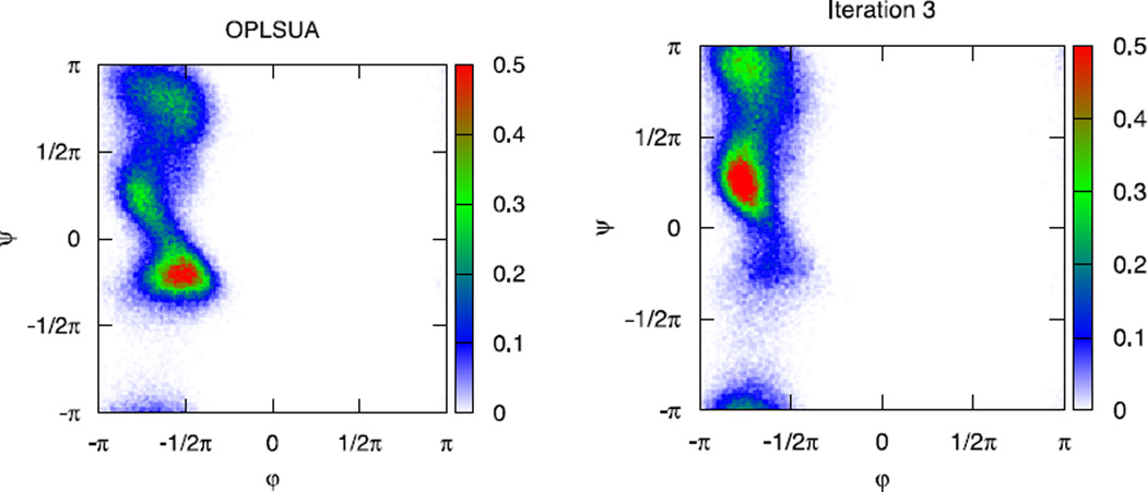
Figure 1 shows the probability density of configurations as a function of (φ,ψ) calculated with the united atom OPLS^5b: all the populated states are located in the region with negative φ (quadrants II and III). The region with highest probability density is in quadrant III and it corresponds to helical states.

Figure 1.

Evolution of the probability density of the dihedral angles (φ, ψ) for alanine dipeptide. The graph on the left shows results obtained with the force field OPLS with united atoms; a propensity to be in helix configuration is indicated by the high-density region in quadrant III. The optimization process reduces the amount of structures in the helical configuration (quadrant III) to the prescribed value (right).

We define our microscopic observable O(x, p) to be the following indicator function:

$$I(\psi )=\begin{array}{cc}\hfill 1\hfill & \hfill -100°\le \psi \le 0°\hfill \\ \hfill 0\hfill & \hfill \mathit{\text{elsewhere}}\hfill \end{array}$$ (11)

The ensemble average of the function I (ψ) is the probability of finding the molecule in the defined region. At 300K approximately 38% of the structures analyzed have ψ-angle that falls in the range −100° to 0°, therefore:

$${\langle I\rangle }_{(OPLSUA,300K)}=0.38$$ (12)

As a proof of principle, we use POP to modify the energy parameters to make the helix region unfavorable. This change does not imply (of course) that the preferred conformation of alanine dipeptide in nature is of extended chain. Nevertheless, it is a useful exercise to illustrate the POP algorithm. We seek to modify the force field in such a way that exactly 10% of the structures lie in the helical region, therefore for the function I (ψ) we set up a target value I_TARGET = 0.1. We will use a single temperature, so the distance function that we use is:

$$\mathrm{\Theta }(\pi )={({\langle I\rangle }_{(\pi ,300K)}-I_{\mathit{\text{TARGET}}})}^2$$ (13)

We minimized Θ (π) as a function of the parameters of the proper torsions and Lennard-Jones interactions. These energy terms are typical targets for optimization. Charges are frequently determined by quantum mechanic calculations and we have them fixed in the present manuscript. The total number of parameters that we consider is 72.

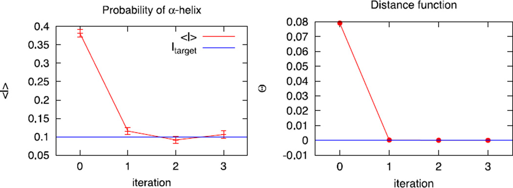
One iteration reduces the target function significantly; after three iterations the Θ (π) distance function is 2 × 10⁻⁵ where 〈I〉_(POP,300K) = 0.106 ± 0.005 and the target was considered achieved (Figure 2).

Figure 2.

Left: Evolution of probability of α-helical configuration as a function of the iteration number. The target value is achieved in 3 iterations. Right: The distance function Θ (π) as a function of the iteration number.

Figure 3 shows the difference in the dynamics of a trajectory obtained with united atom OPLS and one obtained with the last version of the modified potential. When simulated with the original force field the molecule has frequent transitions between the helical state and the extended chain state spending a significant amount of time in the helical state; when simulated with the modified potential the molecule undergoes fewer transitions into the helical state and the amount of time spent in that state is reduced to the one prescribed as a target.

Figure 3.

A comparison between a trajectory obtained with the force field OPLSUA (top) and a trajectory obtained with the last iteration of the modified force field (bottom). Both the trajectories are 1ns long. The original force field shows frequent transition in and out of the helical state whose boundaries (as we defined them) are indicated in blue. The molecule spends ~38% of the time in the helical configuration. The modified force field in the bottom figure shows fewer transitions to the helical state where the molecule spends ~10% of the time.

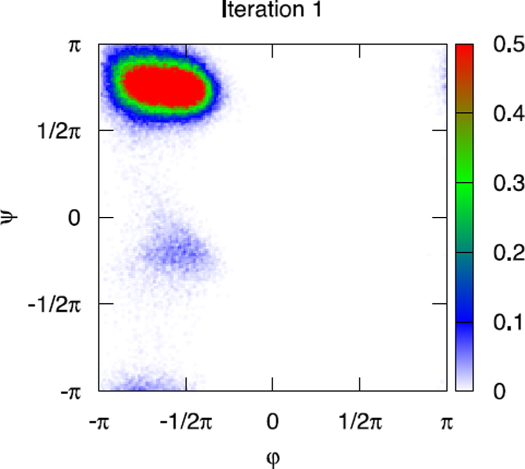
To explore variations in the target function we repeated the POP optimization using a different target; this time instead of reducing the probability of the helical state we increase the probability of the extended chain state. We defined the extended chain state by a range of the ψ-angle (between 90° and 180°); and set I_TARGET = 0.9. The results are shown in Figure 4, the target was essentially achieved with just one optimization step.

Figure 4.

The probability density of states for alanine dipeptide. In this second test we increased the target probability of extended chain to 0.9.

The probability of helix as well as the probability of β-sheet is largely determined by the torsion potential; the sensitivity with respect to the Lennard-Jones parameters is very small and little to no change was made to those parameters.

In MOIL, all possible torsions are generated based on the bond structure that is computed from the system sequence and prior database of amino acid connectivity. In a second step these torsions are assigned values according to the force field at hand. Torsions that do not have contributions to the energy are removed from the list to save computational resources. However, during the optimization it is important to consider also torsions that have no contributions to the current force field but may have one in a refined force field. The POP code was therefore modified to take into account torsion terms with zero coefficients and to compute their parameter derivatives.

Alanine dipeptide has 16 torsions subdivided into 13 torsion types (a torsion type is defined by all four types of atoms in sequence, either in the forward or backward directions). Of the 13 torsion types, 5 torsions are initially set as having no contribution to the energy. Perhaps not surprisingly most of the changes in the force field following POP are in those torsions. POP procedure returns more non-zero torsion coefficients. The stiff torsions (rotations of the amide planes) remain stiff as they should and the free torsions remain relatively soft, even if the coefficients are no longer zero. It is striking that the small, distributed changes of the force field have dramatic effects on the general behavior of the molecule as demonstrated by the density plots.

III.2 WH5

We applied the POP method also to the pentapeptide Ac-WAAAH-NH₂ (WH5) with the aim of reproducing the experimental helical fraction as a function of the temperature. WH5 is forming an α-helical turn efficiently and rapidly¹⁶. WH5 consists of only 5 amino acids, i.e. a minimum number of amino acids to form a complete turn of an α helix. Its secondary structure has been determined by nuclear magnetic resonance (NMR) and circular dichroism (CD) and the kinetics of the helix ↔coil transition has been studied by T-jump experiments^15a. The cited reference reports the far UV CD spectra of WH5 and the derived helical fraction as a function of temperature. The small size of WH5 and its fast kinetics make this molecule the ideal candidate to undergo optimization by POP. The required sampling of conformational space should not be a problem for modern computer hardware and software.

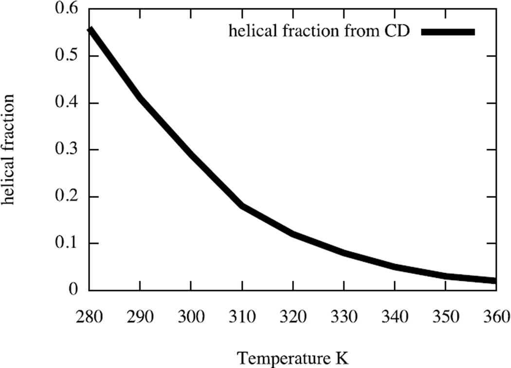
The experimentally determined helical fraction for WH5 is reproduced from the experimental data of ref¹⁶ and is shown in Figure 6 in the temperature range 280–360. In reference¹⁶ the CD spectra was empirically matched against known fingerprints of a helix spectrum. The match provided the plot of helical content in Fig 6. The curve is similar in its overall shape to the melting curve measured for the peptide (AAQAA)₃ by NMR¹⁸. The experimental helical fraction decays from 56% to almost zero. We focus on three temperatures 280 K, 300 K, 320 K and conduct the required simulations as described in section II.4.1

Figure 6.

Experimentally measured fraction of helix conformation. See text for more details.

In general, the average value of the (φ,ψ) angles for the α-helix is peaked near the point (−62°,−41°); we considered an amino acid to be in helical conformation if its backbone dihedral angles fall in a circle of radius 20° from the ideal value. Other definitions are possible. In the Lifson-Roig model emphasis is made on the hydrogen bond and therefore a helix is defined if three sequential amino acids are in the helical state. It is not clear if this is the appropriate definition for CD spectra. We therefore try them both. Below we present the result only for the single-amino acid definition. The use of three (φ,ψ) pairs does not improve the results.

We define our microscopic observable O(x, p) to be the helical fraction:

$$H(x)=\frac{N_{\mathit{\text{helix}}}}{N_{\mathit{\text{total}}}}$$ (14)

where N_helix is the number of amino acids in helical conformation and N_total is the total number of amino acids (5 for WH5).

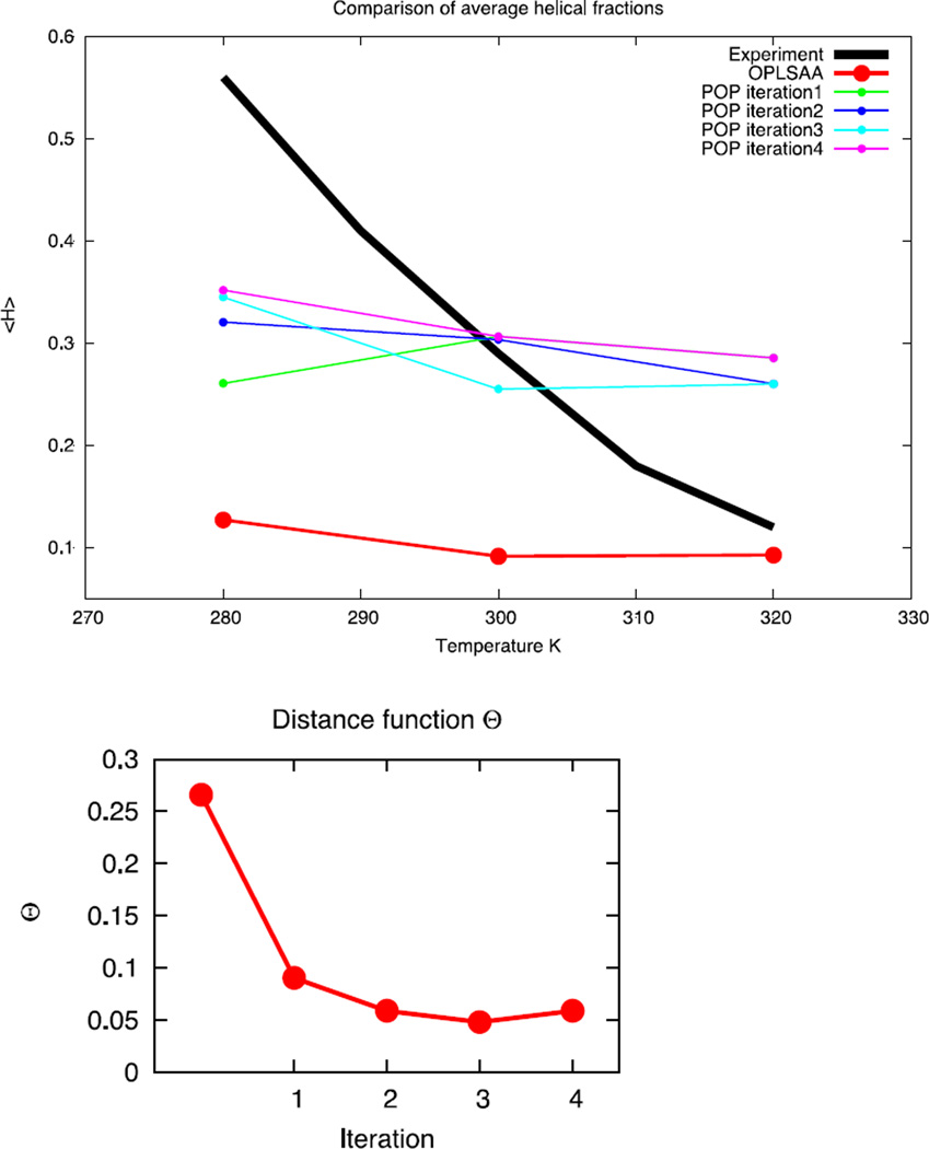
As shown in Figure 7, in this temperature range the simulation with the starting potential gave helical fractions that are at significant variance with experiment.

Figure 7.

Top: A Comparison between the experimental folded fraction (black) and the results obtained from simulations with the OPLSAA force field (red) and optimized POP force fields. Down: Distance function Θ (π) as a function of the iteration

First, the helical fraction calculated from the simulation is less than the experimental value over the complete temperature range. Second, 〈H〉_(OPLSAA,T) doesn’t exhibit the sharp dependence on temperature seen in the experimentally determined curve. The computational curve is almost constant in the range considered.

We defined the target function to be:

$$\mathrm{\Theta }(\pi )={\sum }_i{({\langle H\rangle }_{(\pi ,T_i)}-H_{\text{experiment}}(T_i))}^2$$ (15)

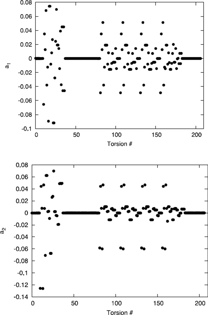
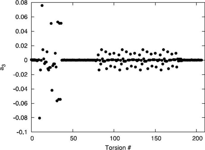
The index i is running over the three temperatures 280, 300 and 320 K. POP optimization was performed on the Van der Waals and torsions parameters to minimize Θ (π); water parameters and charges were left untouched. After the first iteration the helical fraction was significantly improved reproducing the correct value at ~300 K (Figure 7). Three more POP iterations were performed with no substantial improvement; correct temperature dependence (or the overall shape of the melting curve) of the in silico helical fraction could not be achieved. The optimization process acted mostly on the parameters of the 207 torsions present in the molecule, thus confirming the intuitive idea that the helical fraction mostly depends on torsions; not one of the Lennard Jones parameters was modified more the 0.1%.

Remarkably, the changes in torsions parameters were small too. The molecule has 207 torsions subdivided in 97 torsion-types. Of 97 torsion-types just 7 had parameters modified in the range 5–10%, 9 torsions had parameters modified in the range 2–5% while the rest had changes less than 2%. These small, distributed changes in the parameter’s set had a large effect on the helical fraction increasing it by more than a factor 2, Figure 8.

Figure 8.

The difference in the coefficients of the torsion potential (a₁, a₂, a₃) of the OPLS-AA and POP potentials. The differences are small but they cause significant changes in helical content. Note that all torsions are displayed, which means that torsion types that repeat are shown more than once. The zero differences are mostly for side chain torsions.

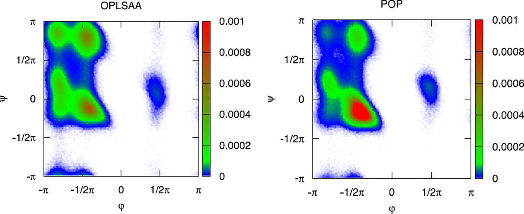
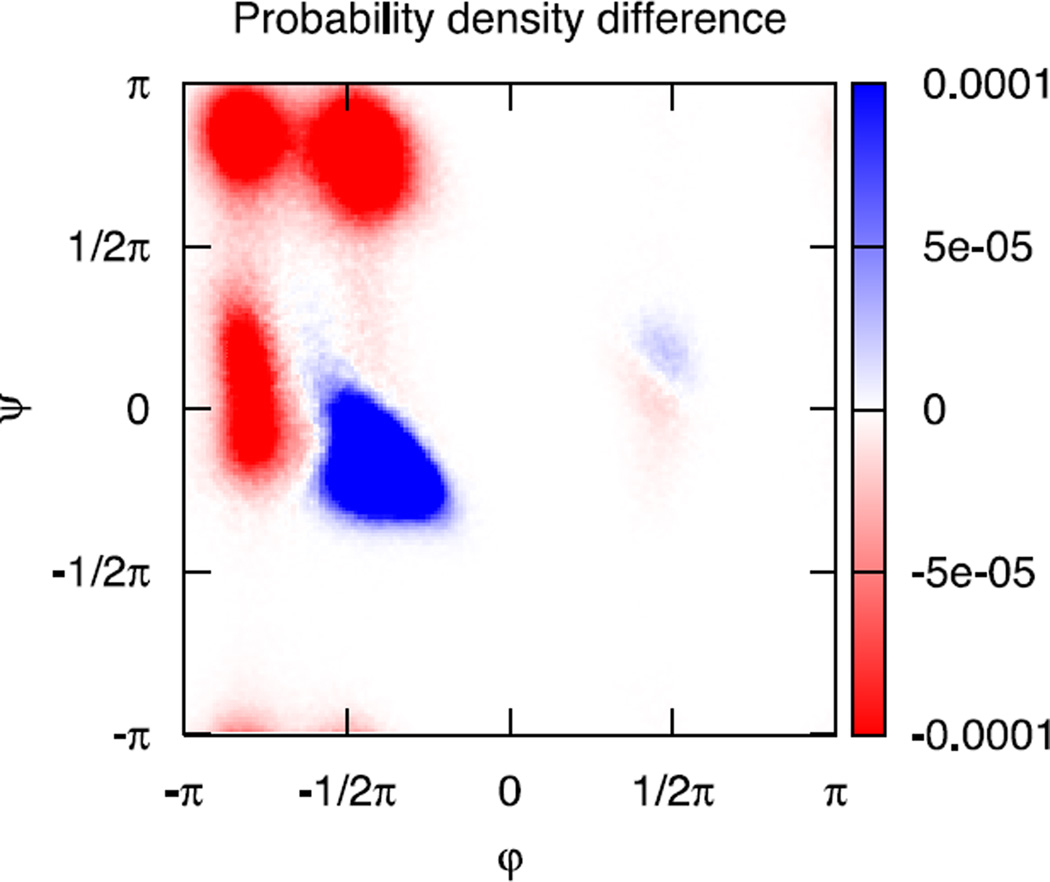
Figure 9 shows the probability density of all the 5 amino acids of WH5 in different positions of the Ramachandran Map. The figure shows a comparison of probability densities for the starting and optimized force fields. The calculation presented is at temperature 300K. The result of the optimization is (as designed) an increased population of helical conformations. The differences between the two probability densities are also reported.

Figure 9.

The three graphs show the probability density of finding any of the amino acids of WH5 in a given configuration defined by its dihedral backbone angles. The top figures show the probability density calculated at 300K from the potential OPLSAA and from the optimized potential POP (iteration 4). The lower figure shows the probability density difference between the two force fields. The probability density is normalized with respect to integration over the dihedrals φ and ψ.

A second attempt to optimize the shape of the melting curve was made by modifying the target function. We focused not on the helical fraction but on its derivative with respect to the temperature. We defined the target function to be:

$$\mathrm{\Theta }(\pi )=\sum _1^2{(D_{(i,\pi )}-D_{(i,\text{experiment})})}^2{D}_{(i,\pi )}=\frac{{\langle H\rangle }_{(\pi .T_{i+1})}-{\langle H\rangle }_{(\pi .T_i)}}{T_{i+1}-T_i}{D}_{(i,\text{experiment})}=\frac{H_{\text{experiment}}\left(T_{i+1}\right)-H_{\text{experiment}}\left(T_i\right)}{T_{i+1}-T_i}$$ (16)

Where T₁, T₂, T₃ are, as before, the temperatures 280,300 and 320 K. We are therefore optimizing the numerical derivative of the helical fraction with respect to the temperature calculated at the two mid-temperatures 290, 310 K.

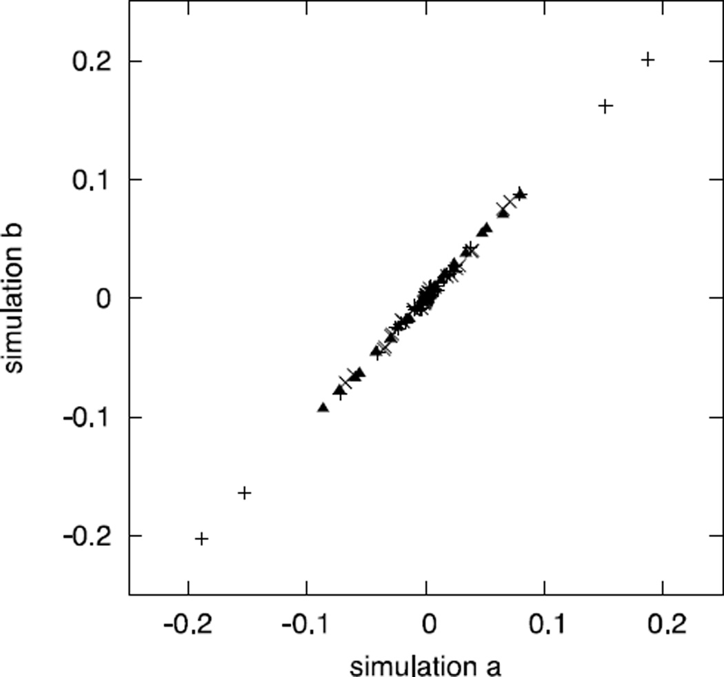
The convergence of the sensitivity was verified using independent simulations. Two molecular dynamics trajectories generate configurations to compute the average and the derivatives independently for each of the trajectories. Figure 10 illustrates the high correlations between the vectors of derivatives suggesting that the calculations of the derivatives indeed converge.

Figure 10.

The gradient of the target function computed by ensemble averages of two simulations (different seeds). We plot the correlation between the two gradients in which every element of the gradient vector is projected onto the axes to obtain the gradient value at each simulation. The high quality linear correlation suggests convergence.

The final value of the target function is Θ = 2.6 × 10⁻⁴. No further improvement in the target function was obtained and the slope was not improving with additional cycles. We concluded that within the error bars of the potential parameters it is not possible to adjust the shape of the melting curve.

Conclusions and Future Directions

In this manuscript we illustrate a combination of sensitivity calculations and direct local optimization of potential parameters for condensed phase simulations. This procedure, called POP, is a potentially useful approach for fine-tuning an energy function for applications in which statistical mechanic averages are compared with experimental measurements. The advantage of the proposed approach is that it can handle a large number of parameters in a single automated calculation. This is not to say that human decisions are completely factored out. Especially for cases in which multiple experimental observables are of interest we expect to have weight coefficients for a sum of measured observables $\mathrm{\Theta }=\sum _i{w}_i{(\langle O_i\rangle -O_{\text{exp},i})}^2$ where the weights, w_i, are determined by the user. Experimental uncertainties as well as the importance of a particular observable for future projects impact the choice of the weights.

Another direction that we did not consider in the present investigation is of stochastic sampling, searching for multiple solutions of parameter sets and potentially a global minimum. In the current investigation we focused on one observable and a minimal change to the parameters. However, one may apply the same protocol to a large number of observables (weighted appropriately) and a large number of parameters to be modified in a substantial way. The feasibility of conducting converged statistical mechanic simulations on moderately complex molecules makes the present approach attractive.

Finally we comment on the results for the peptide WH5 and their implications. We found that the helical content was a highly sensitive function of the backbone torsion parameters. In a way this is good news since the optimization of existing potentials to obtain the correct helical content is not difficult, provided that the direction of parameter changes is chosen correctly. Only minute adjustments in the potential parameters are required in order to bring the system to the correct conformations in equilibrium. Since the changes in the parameters are small it is likely that other observables will not be affected. A concern is however of transferability. If indeed such small adjustment in parameters cause such large shift in helical content, it is likely that transferability to other peptide systems (and proteins) would be hard to achieve since different peptides may require other small adjustments.

Another interesting observation in the simulation of WH5 is our inability to reproduce the melting curve of the peptide. These widely used experimental curves to determine stability energies and entropies of protein folding are insensitive functions of the parameters at hand. In fact, we gave up on the optimization since the procedure we use did not seem to make progress. We stress that our failure is relevant also to single temperature properties since quantities like entropy are related to the derivatives of the free energy and hence are incorrect.

The failure of our efforts to produce a potential that correctly predicts the melting curve discourages us from testing it on other systems. This negative result is supported by other attempts in the field to understand the unusual stability of short helices and to adjust force fields to reproduce this experimental observation. Arguments were made in the past that interactions with charged side chains add to the strong co-operativity of the helix¹⁹. The current optimization does not include all types of side chains and hence our exploration is limited. Nevertheless, some coupling of the backbone conformation is observed for the side chain torsion of tryptophan, supporting general interaction of side chains to backbone.²¹

A number of extensions to the standard force field were proposed in the past. First, the water model (which we held fixed) may be inappropriate for a range of temperatures. Water models as TIP4P²² and TIP5P²³, as well as a polarizable water model²⁴ are of significant promise since they better describe water properties and water anomalies. An interesting study was published by Best and Mittal²⁵ that illustrated the complexity of the task. The use of TIP4P/2005²⁶ showed moderate improvement after the peptide potential was re-parameterized. Hence the peptide parameters are strongly coupled to the water model, which in most force fields are fitted against TIP3P or a similar model. Second, adjustments to the backbone torsion potentials were made. The CMAP approach has shown promise and the progress is encouraging^{21, 27}. In the CMAP approach a coupling between the (φ,ψ) dihedral angles is introduced, taking into account experimentally determined protein structures. This term is added to the usual Fourier expansion of the torsion energies that considers a torsion at a time. Another extension was proposed by Sakae and Okamoto²⁸ in which the torsion energy is made dependent on the amino acid type. The last approach, however, was not illustrated to improve peptide-melting curves. Third, polarizable force fields²⁹ may also play a future role, and their evaluation is desired.

Finally we make a cautionary remark. While our results support the designs beyond the standard force field, they are a conjecture and not a proof. Our sampling of parameter space is incomplete. The optimization is based on a local minimization in which a nearby optimum of the target function is searched with a minimal change in the parameter values. The parameter space is rather smooth (especially compared to the coordinate space) since the energy dependence on the parameters that we optimize is either linear (torsion) or quadratic (Lennard Jones). For simple (quadratic) target functions the local minimization is exact. However, the Boltzmann factor makes the target function more complex and if exploration of multiple minima is required we will miss it.

Figure 5.

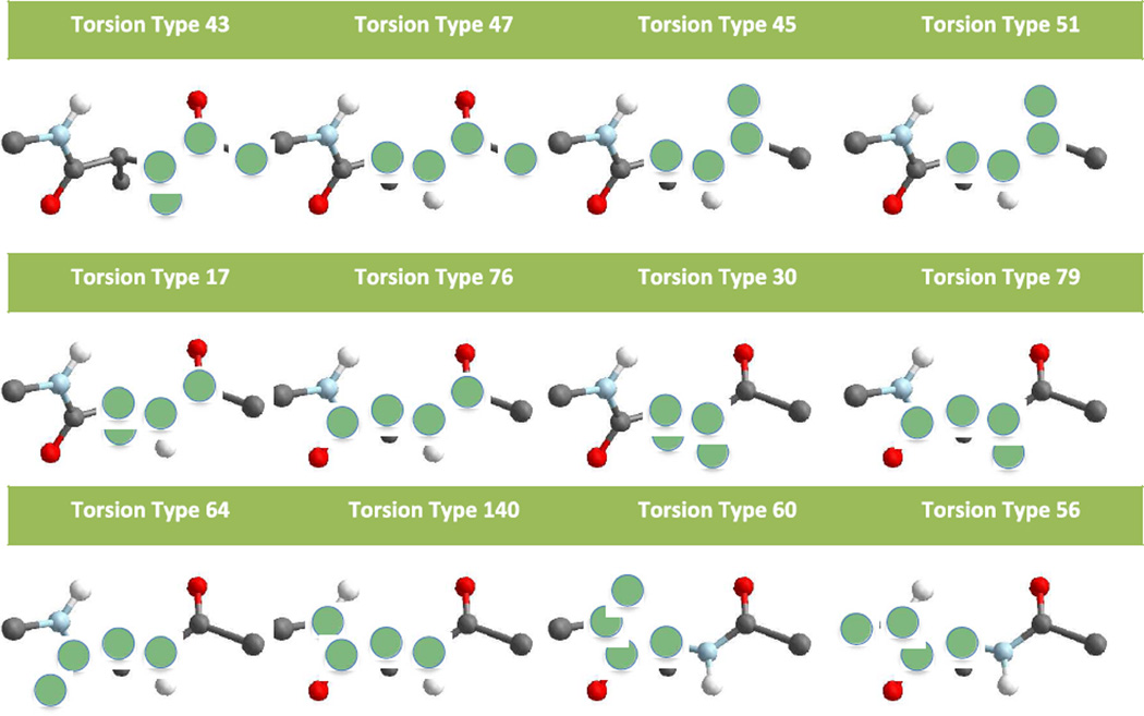
Sampled torsions. In green circles we show the four atoms that are active in a particular torsion. Sometimes torsion parameters are modeled only according to the central two atoms. Here we take the broader view and consider torsions with even one of the four atoms different as distinct.

Table 2.

Coefficients in the expansion of a torsion energy term α $U_{\alpha }\left(\varphi \right)=\sum _n{a}_{n,a}[1+\text{cos}(n·\varphi -{\delta }_{n,a}\left)\right]$. Only the coefficients a_n are optimized. δ_n is fixed at π. Sample of torsion types, their atom types, and their corresponding indices are shown in Figure 5.

Torsion Type		Starting parameters			POP
	a1	a2	a3	a1	a2	a3
43	0.0000	2.5000	0.0000	−0.0001	2.4998	−0.0005
47	0.0000	2.5000	0.0000	0.0000	2.4999	0.0002
45	0.0000	2.5000	0.0000	0.0000	2.4999	0.0004
51	0.0000	2.5000	0.0000	0.0000	2.4999	−0.0003
17	0.0000	0.0000	0.0000	0.0586	−0.1096	0.0305
76	0.0000	0.0000	0.0000	−0.0682	0.0873	0.0434
30	0.0000	0.0000	0.0000	−0.0604	−0.1110	−0.0289
79	0.0000	0.0000	0.0000	0.0704	0.0883	−0.0408
64	0.0000	0.0000	0.1000	0.2167	−0.0354	0.0375
140	0.0000	0.0000	0.0000	−0.2157	0.2981	0.0548
60	0.0000	2.5000	0.0000	0.0000	2.4999	−0.0002
56	0.0000	2.5000	0.0000	0.0000	2.5001	−0.0002
55	0.0000	2.5000	0.0000	0.0000	2.4999	0.0005

References

- 1.Frenkel D, Berend S. Understanding Moelcular Simulation: From algorithms to applications. San Diego: Academic Press; 1996. [Google Scholar]
- 2.Abrams JB, Tuckrman ME, Martyna GJ. a chapter. In: Ferrario M, Ciccotti G, Binder K, editors. Computer simulations in condensed matter: From materials to chemical biology. Vol 1. Berin: Springer; 2006. pp. 139–192. [Google Scholar]
- 3.Brooks BR, Brooks CL, Mackerell AD, Nilsson L, Petrella RJ, Roux B, Won Y, Archontis G, Bartels C, Boresch S, Caflisch A, Caves L, Cui Q, Dinner AR, Feig M, Fischer S, Gao J, Hodoscek M, Im W, Kuczera K, Lazaridis T, Ma J, Ovchinnikov V, Paci E, Pastor RW, Post CB, Pu JZ, Schaefer M, Tidor B, Venable RM, Woodcock HL, Wu X, Yang W, York DM, Karplus M. CHARMM: The Biomolecular Simulation Program. J. Comput. Chem. 2009;30(10):1545–1614. doi: 10.1002/jcc.21287. [DOI] [PMC free article] [PubMed] [Google Scholar]
- 4.Case DA, Cheatham TE, Darden T, Gohlke H, Luo R, Merz KM, Onufriev A, Simmerling C, Wang B, Woods RJ. The AMBER biomolecular simulation programs. J. Comput. Chem. 2005;26(16):1668–1688. doi: 10.1002/jcc.20290. [DOI] [PMC free article] [PubMed] [Google Scholar]
- 5.(a) Kaminski G, Friesner R, Tirado-Rives J, Jorgensen WL. Evaluation and reparameterization of the OPLS-AA force field for proteins via comparison with accurate quantum chemical calculations on peptides. J. Phys. Chem. B. 2001;105(28):6474–6487. [Google Scholar]; (b) Jorgensen WL, Tiradorives J. The OPLS potential functions for proteins - energy minimizations for crystals of cyclic-peptides and crambin. J. Am. Chem. Soc. 1988;110(6):1657–1666. doi: 10.1021/ja00214a001. [DOI] [PubMed] [Google Scholar]
- 6.Jorgensen WL, Chandrasekhar J, Madura JD, Impey RW, Klein ML. Comparison of simple potential functions for simulating liquid water. J. Chem. Phys. 1983;79(2):926–935. [Google Scholar]
- 7.Nocedal J, Wright SJ. Numerical Optimization. New York: Springer; 1999. [Google Scholar]
- 8.(a) Chen AA, Pappu RV. Parameters of monovalent ions in the AMBER-99 forcefield: Assessment of inaccuracies and proposed improvements. J. Phys. Chem. B. 2007;111(41):11884–11887. doi: 10.1021/jp0765392. [DOI] [PubMed] [Google Scholar]; (b) Hornak V, Abel R, Okur A, Strockbine B, Roitberg A, Simmerling C. Comparison of multiple amber force fields and development of improved protein backbone parameters. Proteins: Struct. Funct. Bioinf. 2006;65(3):712–725. doi: 10.1002/prot.21123. [DOI] [PMC free article] [PubMed] [Google Scholar]
- 9.(a) Ruymgaart AP, Cardenas AE, Elber R. MOIL-opt: Energy-Conserving Molecular Dynamics on a GPU/CPU System. J. Chem. Theory Comput. 2011;7(10):3072–3082. doi: 10.1021/ct200360f. [DOI] [PMC free article] [PubMed] [Google Scholar]; (b) Elber R, Roitberg A, Simmerling C, Goldstein R, Li HY, Verkhivker G, Keasar C, Zhang J, Ulitsky A. Moil a program for simulations of macrmolecules. Comput. Phys. Commun. 1995;91(1–3):159–189. [Google Scholar]
- 10.Weiner SJ, Kollman PA, Case DA, Singh UC, Ghio C, Alagona G, Profeta S, Weiner P. A new force-field for molecular mechanical simulation of nucleic-acids and proteins. J. Am. Chem Soc. 1984;106(3):765–784. [Google Scholar]
- 11.Tuckerman M, Berne BJ, Martyna GJ. Reversible multiple time scale molecular-dynamics. J. Chem. Phys. 1992;97(3):1990–2001. [Google Scholar]
- 12.(a) Weinbach Y, Elber R. Revisiting and parallelizing SHAKE. J. Comput. Phys. 2005;209(1):193–206. [Google Scholar]; (b) Ruymgaart AP, Elber R. Revisiting Molecular Dynamics on a CPU/GPU System: Water Kernel and SHAKE Parallelization. J. Chem. Theory Comput. 2012;8(11):4624–4636. doi: 10.1021/ct300324k. [DOI] [PMC free article] [PubMed] [Google Scholar]
- 13.Ryckaert JP, Ciccotti G, Berendsen HJC. Numerical integration of cartesian equations of motion of a system with constraints - molecular dynamics of N-alkanes. J. Comput. Phys. 1977;23(3):327–341. [Google Scholar]
- 14.Essmann U, Perera L, Berkowitz ML, Darden T, Lee H, Pedersen LG. A smooth particle mesh ewald method. J. Chem. Phys. 1995;103(19):8577–8593. [Google Scholar]
- 15.(a) Lin MM, Mohammed OF, Jas GS, Zewail AH. Speed limit of protein folding evidenced in secondary structure dynamics. Proc. Natl. Acad. Sci. U. S. A. 2011;108(40):16622–16627. doi: 10.1073/pnas.1113649108. [DOI] [PMC free article] [PubMed] [Google Scholar]; (b) Hegefeld WA, Chen SE, DeLeon KY, Kuczera K, Jas GS. Helix Formation in a Pentapeptide Experiment and Force-field Dependent Dynamics. J. Phys. Chem. A. 2010;114(47):12391–12402. doi: 10.1021/jp102612d. [DOI] [PubMed] [Google Scholar]; (c) Mohammed OF, Jas GS, Lin MM, Zewail AH. Primary Peptide Folding Dynamics Observed with Ultrafast Temperature Jump. Angew. Chem. Int. Ed. Engl. 2009;48(31):5628–5632. doi: 10.1002/anie.200900513. [DOI] [PMC free article] [PubMed] [Google Scholar]
- 16.Jas GS, Hegefeld WA, Majek P, Kuczera K, Elber R. Experiments and Comprehensive Simulations of the Formation of a Helical Turn. J. Phys. Chem. B. 2012;116(23):6598–6610. doi: 10.1021/jp211645s. [DOI] [PMC free article] [PubMed] [Google Scholar]
- 17.(a) Earl DJ, Deem MW. Parallel tempering: Theory, applications, and new perspectives. Phys. Chem. Chem. Phys. 2005;7(23):3910–3916. doi: 10.1039/b509983h. [DOI] [PubMed] [Google Scholar]; (b) Sugita Y, Okamoto Y. Replica-exchange molecular dynamics method for protein folding. Chem. Phys. Lett. 1999;314(1–2):141–151. [Google Scholar]; (c) Kirmizialtin S, Elber R. Computational Exploration of Mobile Ion Distributions around RNA Duplex. J. Phys. Chem. B. 2010;114(24):8207–8220. doi: 10.1021/jp911992t. [DOI] [PMC free article] [PubMed] [Google Scholar]
- 18.Shalongo W, Dugad L, Stellwagen E. Distribution of helicity within the model peptide acetyl(AAQAA)3amide. J. Am. Chem. Soc. 1994;116(18):8288–8293. [Google Scholar]
- 19.(a) Vila JA, Ripoll DR, Scheraga HA. Physical reasons for the unusual alpha-helix stabilization afforded by charged or neutral polar residues in alanine-rich peptides. Proc. Natl. Acad. Sci. U. S. A. 2000;97(24):13075–13079. doi: 10.1073/pnas.240455797. [DOI] [PMC free article] [PubMed] [Google Scholar]; (b) Garcia AE, Sanbonmatsu KY. alpha-Helical stabilization by side chain shielding of backbone hydrogen bonds. Proc. Natl. Acad. Sci. U. S. A. 2002;99(5):2782–2787. doi: 10.1073/pnas.042496899. [DOI] [PMC free article] [PubMed] [Google Scholar]
- 20.Best RB, Hummer G. Optimized Molecular Dynamics Force Fields Applied to the Helix-Coil Transition of Polypeptides. J. Phys. Chem. B. 2009;113(26):9004–9015. doi: 10.1021/jp901540t. [DOI] [PMC free article] [PubMed] [Google Scholar]
- 21.Best RB, Zhu X, Shim J, Lopes PEM, Mittal J, Feig M, MacKerell AD. Optimization of the Additive CHARMM All-Atom Protein Force Field Targeting Improved Sampling of the Backbone phi, psi and Side-Chain chi(1) and chi(2) Dihedral Angles. J. Chem. Theory Comput. 2012;8(9):3257–3273. doi: 10.1021/ct300400x. [DOI] [PMC free article] [PubMed] [Google Scholar]
- 22.Jorgensen WL, Madura JD. Temperature and size dependence for monte-carlo simulations of tip4p water. Mol. Phys. 1985;56(6):1381–1392. [Google Scholar]
- 23.Mahoney MW, Jorgensen WL. A five-site model for liquid water and the reproduction of the density anomaly by rigid, nonpolarizable potential functions. J. Chem. Phys. 2000;112(20):8910–8922. [Google Scholar]
- 24.Ren PY, Ponder JW. Temperature and pressure dependence of AMOEBA water model. J. Phys. Chem. B. 2004;108(35):13427–13437. [Google Scholar]
- 25.Best RB, Mittal J. Protein Simulations with an Optimized Water Model: Cooperative Helix Formation and Temperature-Induced Unfolded State Collapse. J. Phys. Chem. B. 2010;114(46):14916–14923. doi: 10.1021/jp108618d. [DOI] [PubMed] [Google Scholar]
- 26.Abascal JLF, Vega C. A general purpose model for the condensed phases of water: TIP4P/2005. J. Chem. Phys. 2005;123(23) doi: 10.1063/1.2121687. [DOI] [PubMed] [Google Scholar]
- 27.(a) Mackerell AD, Feig M, Brooks CL. Extending the treatment of backbone energetics in protein force fields: Limitations of gas-phase quantum mechanics in reproducing protein conformational distributions in molecular dynamics simulations. J. Comput. Chem. 2004;25(11):1400–1415. doi: 10.1002/jcc.20065. [DOI] [PubMed] [Google Scholar]; (b) Best RB, Mittal J, Feig M, MacKerell AD. Inclusion of Many-Body Effects in the Additive CHARMM Protein CMAP Potential Results in Enhanced Cooperativity of alpha-Helix and beta-Hairpin Formation. Biophys. J. 2012;103(5):1045–1051. doi: 10.1016/j.bpj.2012.07.042. [DOI] [PMC free article] [PubMed] [Google Scholar]
- 28.Sakae Y, Okamoto Y. Amino-acid-dependent main-chain torsion-energy terms for protein systems. J. Chem. Phys. 2013;138(6) doi: 10.1063/1.4774159. [DOI] [PubMed] [Google Scholar]
- 29.(a) Wu JC, Chattree G, Ren PY. Automation of AMOEBA polarizable force field parameterization for small molecules. Theor. Chem. Acc. 2012;131(3) doi: 10.1007/s00214-012-1138-6. [DOI] [PMC free article] [PubMed] [Google Scholar]; (b) Baker CM, Anisimov VM, MacKerell AD. Development of CHARMM Polarizable Force Field for Nucleic Acid Bases Based on the Classical Drude Oscillator Model. J. Phys. Chem. B. 2011;115(3):580–596. doi: 10.1021/jp1092338. [DOI] [PMC free article] [PubMed] [Google Scholar]