RubiX: Combining Spatial Resolutions for Bayesian Inference of Crossing Fibers in Diffusion MRI

Abstract

The trade-off between signal-to-noise ratio (SNR) and spatial specificity governs the choice of spatial resolution in magnetic resonance imaging (MRI); diffusion-weighted (DW) MRI is no exception. Images of lower resolution have higher signal to noise ratio, but also more partial volume artifacts. We present a data-fusion approach for tackling this trade-off by combining DW MRI data acquired both at high and low spatial resolution. We combine all data into a single Bayesian model to estimate the underlying fiber patterns and diffusion parameters. The proposed model, therefore, combines the benefits of each acquisition. We show that fiber crossings at the highest spatial resolution can be inferred more robustly and accurately using such a model compared to a simpler model that operates only on high-resolution data, when both approaches are matched for acquisition time.

I. Introduction

WHITE matter tractography has been amongst the most commonly-used applications of diffusion-weighted (DW) magnetic resonance imaging (MRI), allowing the study of brain structural connectivity [1]–[3]. A challenging problem in tractography is the resolution of complex fiber patterns, such as fiber crossings; this has drawn a lot of attention over the recent years (see [4] for a review). A plethora of methods have been proposed that rely on different sampling patterns of q-space, the Fourier-conjugate space of the 3D diffusion displacements.

All the proposed techniques follow a standard, natural choice for approaching the problem; utilizing a dataset acquired at a single spatial resolution. Therefore, they inherently have the limitations imposed by the associated spatial resolution grid. The trade-off between reduced signal-to-noise ratio (SNR) and increased spatial specificity governs the choice of spatial resolution in magnetic resonance imaging [5]. Benefits from improvements in either of those parameters have been shown. For instance, high SNR values are beneficial for robust estimation of tissue microstructure properties from the DW MRI signal, e.g., [6]–[9]. On the other hand, high spatial resolution reduces partial volume effects and allows exquisite tissue details to be revealed, as has been shown from postmortem acquisitions [10]. Thus, an approach that combines multiple spatial resolutions could intuitively combine the benefits. We introduce and explore here a novel framework for combining multiple spatial resolutions during fiber orientation estimation.

The methods proposed so far utilize a single spatial resolution and can be categorized according to their q-space sampling patterns. Single-shell, high-angular resolution diffusion imaging (HARDI) methods utilize acquisitions that sample, relatively densely, a single sphere in q-space. Parametric [11]–[14] or nonparametric approaches [6], [15]–[19] exist that either estimate directly the dominant fiber orientations within each voxel or reconstruct orientation distribution functions (ODFs) on the sphere. A different group of methods use a more generic q-space sampling, in the form of multiple concentric spheres [20]–[22] or a Cartesian grid [23], [24] (collectively termed here as multishell). These methods aim to tackle the trade-off between increased angular specificity and reduced SNR, as we move away from the centre of q-space in diffusion MRI. They have been shown to be more sensitive than the single-shell approaches in revealing detailed features of the underlying fiber pattern [17], [22], [25].

Our proposed framework is different in spirit than the above approaches. We assume that an object has been scanned at different spatial resolutions; the high-resolution acquisitions offer spatial specificity, but low SNR, while the low-resolution ones offer much higher SNR, but are more prone to partial volume. We combine all resolutions into a single Bayesian model to estimate the underlying fiber patterns at the highest of the available resolutions. The motivation comes from the fact that the same fiber pattern will be imaged differently at different resolutions. By unifying the information across resolutions we combine features offered by each acquisition and tackle the trade-off between increased spatial specificity and reduced SNR.

The RubiX (Resolutions Unified for Bayesian Inference of Crossings) generative model represents a data-fusion framework, where data from all resolutions are combined through a spatial and a local model. Priors on the model parameters impose some spatial regularization constraints that assist model identifiability when the high resolution data are of very low SNR. The generative model is inverted using Markov-Chain Monte-Carlo (MCMC) and the posterior distribution of the parameters is estimated. We show that fiber crossings at the highest spatial resolution can be inferred more robustly compared to an approach that uses only high-resolution data, when both approaches are matched for acquisition time.

II. Methods

A. Overview of the Rubix Generative Model

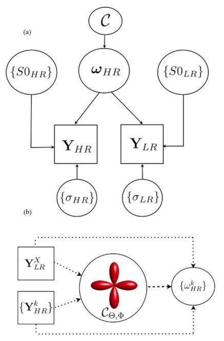
Let us assume that an object has been scanned at two different spatial resolutions. The aim is to construct a model that utilizes both datasets and estimates parameters at the highest spatial resolution. Let ${\mathbf{Y}}_{\mathrm{LR}}=\left\{y_{\mathrm{LR}}^{\mathit{XM}}\right\}$ be the set of all measurements at a low-resolution grid, across all voxels X = 1 : K_LR and diffusion-sensitizing directions¹ M = 1 : M_LR. Similarly, let ${\mathbf{Y}}_{\mathrm{HR}}=\left\{y_{\mathrm{HR}}^{\mathit{xm}}\right\}$ be the set of measurements at a high-resolution grid, across all voxels x = 1 : K_HR and directions m = 1 : M_HR. Then, the mechanism can be understood through the graphical generative model of Fig. 1(a). The graph shows that the data at both resolutions are generated by a model parameterized by ω_HR, a set of voxel-wise parameters at the higher resolution grid. These parameters are restricted by the prior hyper-parameters $\mathcal{C}$. Different noise levels σ and baseline signals S0 are used for each acquisition.

Fig. 1.

(a) RubiX graphical model illustrates how datasets Y at both resolution grids are generated by a set of model parameters ω_HR specified at the high resolution grid. The model incorporates different noise levels σ and baseline levels S0 for each grid. A group of prior hyperparameters $\mathcal{C}$ influence the data generation at both resolutions. Notice that during the inversion of this model, all parameters ω, S0, σ and $\mathcal{C}$ are treated as unknowns estimated from the measured Y_HR and Y_LR. (b) Simplistic graphical sketch that shows how the orientation conditional priors ${\mathcal{C}}_{\Theta ,\Phi }$ are estimated from the data and influence subsequently the estimation of parameters at the HR. As the priors are common to subgroups of k HR voxels intersected by the same LR voxel X, they are influenced more by the way fiber patterns are depicted at LR.

We treat ω_HR as the set of parameters of local models that generate the predicted DW signal $S_{\mathrm{HR}}^{\mathit{xm}}$ at each voxel x of the high-resolution grid. Assuming that the two spatial grids are registered to each other, we can apply a partial volume model to relate these parameters to the predicted signal $S_{\mathrm{LR}}^{\mathit{XM}}$ at the low-resolution grid. The partial volume model that predicts the signal for a voxel X is

$$S_{\mathrm{LR}}^{\mathit{XM}}=\sum _{k=1}^K{\alpha }_k{S}_{\mathrm{HR}}^{\mathit{kM}}$$ (1)

with index k describing the K HR voxels that intersect voxel X, each with a volume fraction α_k. The above model predicts that the signal at a LR voxel X and direction M is a weighted sum of the signals predicted at the intersected HR voxels. It can be used in conjunction with a local model at the high-resolution voxels to relate parameters ω_HR to both LR and HR measurements.

The above model assumes that all timing parameters (echo time TE, repetition time TR) are the same for the LR and HR acquisitions. A more flexible representation of the data would be

$$\frac{S_{\mathrm{LR}}^{\mathit{XM}}}{S{0}_{\mathrm{LR}}^X}=\sum _{k=1}^K{\alpha }_k\frac{S_{\mathrm{HR}}^{\mathit{kM}}}{S{0}_{\mathrm{HR}}^k}$$ (2)

with S0’s being the baseline signals without diffusion-weighting at each acquisition. The above model predicts that the signal attenuation at a LR voxel X and direction M is a weighted sum of the signal attenuations predicted at the intersected HR voxels. This is an approximation that allows greater flexibility in the datasets to be combined without having to consider T1 and T2-related effects. It is valid under the assumption of relative constant proton density and relaxation times across a small neighborhood of K HR voxels and will be used in this study.

The partial volume models assume arbitrary low and high resolutions to be combined. For simplicity of illustration and implementation, we will assume from now on an integer volume ratio of LR and HR voxels. This implies α_k = 1/K and that each HR voxel x intersects only one LR voxel X; or that K HR voxels fit perfectly within one LR voxel (voxel sizes of 3 × 3 × 3 mm³ and 1.5 × 1.5 × 1.5 mm³ for instance).

B. Local Model

The ball & stick model [7], [12] is used to model the DW signal at every HR voxel x. The model parameters of all voxels x give the set ω_HR. The signal after the application of the m^th diffusion-sensitizing gradient with direction g_m and b value b_m is modelled as

$$\begin{array}{cc}\hfill S_{\mathrm{HR}}^{\mathit{xm}}=S{0}_{\mathrm{HR}}^x& [\left(1-\sum _{n=1}^N{f}_n\right)\exp (-b_{m}d)\phantom{]}\hfill \\ \hfill & +\phantom{[}\sum _{n=1}^N{f}_n\exp (-b_{m}d{\left({\mathbf{g}}_m^T{\mathbf{v}}_n\right)}^2)]\hfill \end{array}$$ (3)

with d the apparent diffusivity and f_n ∈ [0,1] the volume fraction of the anisotropic compartment with orientation v_n = [sinθ_ncosϕ_n sinθ_nsinϕ_n cosθ_n]^T, θ_n ∈ [0,π] and ϕ_n ∈ [0, 2π).

C. Bayesian Inference

Since we have assumed dependence only between a LR voxel X and the set of K HR voxels that X is intersected by, the generative model of the data ${\mathbf{Y}}_X=({\mathbf{Y}}_{\mathrm{LR}}^X,\{{\mathbf{Y}}_{\mathrm{HR}}^k\left\}\right)$ given all the parameters $\Omega =\left(\right\{{\omega }_{\mathrm{HR}}^k\},\{{\sigma }_{\mathrm{HR}}^k\},\{S{0}_{\mathrm{HR}}^k\},{\sigma }_{\mathrm{LR}}^X,S{0}_{\mathrm{LR}}^X)$, k = 1 : K can be expressed by the following likelihood function (the superscript X is assumed and will be omitted from now on):

$$\begin{array}{cc}\hfill P(\mathbf{Y}\mid \Omega )& =P({\mathbf{Y}}_{\mathrm{LR}}\mid \Omega )\prod _{k=1}^{K}P({\mathbf{Y}}_{\mathrm{HR}}^k\mid \Omega )\hfill \\ \hfill & =\prod _{M=1}^{M_{\mathrm{LR}}}P(y_{\mathrm{LR}}^M\mid \Omega )\prod _{k=1}^K\prod _{m=1}^{M_{\mathrm{HR}}}P(y_{\mathrm{HR}}^{\mathit{km}}\mid \Omega ).\hfill \end{array}$$ (4)

Using the partial volume (2) and the local models (3) and under the assumption of additive, zero-mean, Gaussian noise, we have

$$\begin{array}{cc}\hfill P(y_{\mathrm{LR}}^M\mid \Omega )& \sim \mathcal{N}(S_{\mathrm{LR}}^M,{\sigma }_{\mathrm{LR}}^2)\hfill \\ \hfill P(y_{\mathrm{HR}}^{\mathit{km}}\mid \Omega )& \sim \mathcal{N}(S_{\mathrm{HR}}^{\mathit{km}},{\sigma }_{\mathrm{HR}}^2).\hfill \end{array}$$ (5)

Inference on the parameters Ω of this model, given the data, can be performed individually for each LR voxel X (and its intersecting HR voxels {x^k}), as the voxels are assumed to be independent. We follow the formalism of [7], [12] to construct a random-walk, Metropolis–Hastings sampler and compute the posterior distribution of the model parameters. Using Bayes’ theorem: P(Ω|Y) ∝ P(Y|Ω) P(Ω), where P(Ω) is the unconditional prior distribution of the model parameters. If the prior is conditional on hyper-prior parameters $\mathcal{C}$ (as shown in Fig. 1), then

$$\begin{array}{cc}\hfill P(\Omega ,\mathcal{C}\mid \mathbf{Y})\propto & P(\mathbf{Y}\mid \Omega )P(\Omega \mid \mathcal{C})P\left(\mathcal{C}\right),\text{with}\hfill \\ \hfill P(\Omega \mid \mathcal{C})P\left(\mathcal{C}\right)\propto & P\left({\sigma }_{\mathrm{LR}}\right)P\left(S{0}_{\mathrm{LR}}\right)P\left({\mathcal{C}}_{\Theta ,\Phi }\right)P\left({\mathcal{C}}_d\right)P\left({\mathcal{C}}_F\right)\hfill \\ \hfill & \times \prod _{k=1}^K(P\left({\sigma }_{\mathrm{HR}}^k\right)P\left(S{0}_{\mathrm{HR}}^k\right)P({\Theta }^k,{\Phi }^k\mid {\mathcal{C}}_{\Theta ,\Phi })\phantom{)}\hfill \\ \hfill & \phantom{(}P(d^k\mid {\mathcal{C}}_d)P(F^k\mid {\mathcal{C}}_F)).\hfill \end{array}$$ (6)

In the previous equation, $P(\Omega \mid \mathcal{C})$ is the conditional prior of the parameters of interest Ω on hyperparameters $\mathcal{C}$ and $P\left(\mathcal{C}\right)$ is the unconditional prior of the hyperparameters. Conditional priors are employed for the set of orientation parameters (Θ Φ), the diffusivities d and the volume fractions F (we use capital letters to denote the set of all N orientations (θ, ϕ_n) and all volume fractions f_n within an HR voxel k). These priors are explicitly described in the following sections. For the σ and S0 parameters, unconditional priors are chosen, so that they have the smallest possible influence on the posterior distribution

$$P\left(S{0}_{\mathrm{LR}}\right)\sim \mathcal{U}(0,\infty )\text{and}P\left(S{0}_{\mathrm{HR}}\right)\sim \mathcal{U}(0,\infty ).$$ (7)

As we are not interested in estimating the σ parameters, reference (uninformative) priors are used so that they can be integrated out. See Appendix A for the derivations.

The conditional priors are chosen to indirectly unify orientation, volume fraction and diffusivity estimates across the two spatial resolutions. They are imposed on parameters of the local models. The hyper-parameters of these priors are common to all HR voxels {x^k} intersected by the LR voxel X and are also estimated from the data. Therefore, they mostly reflect fiber patterns as depicted at LR and the data at the low-resolution grid. The model allows the values of these hyper-parameters to further propagate as constraints on the estimation of the model parameters at the high-resolution grid. Fig. 1(b) shows a simplistic sketch of the two ways data influence parameter estimation: either directly or indirectly through the conditional priors. The indirect path promotes an identifiable and spatially coherent solution, particularly useful when the HR data are highly contaminated by noise. The direct path is described by the likelihood function. In the following sections, we briefly describe each of the conditional priors.

D. Conditional Prior on Orientations

We use a mixture of L Watson distributions [26], each with an unknown mode μ_l and concentration k_l, as a prior on each modelled fiber orientation v = (θ, ϕ)

$$\begin{array}{cc}\hfill P(\theta ,\varphi \mid {\mathcal{C}}_{\Theta ,\Phi })& =P(\theta ,\varphi \mid \{{\mu }_l,{\kappa }_l\left\}\right)\hfill \\ \hfill & \propto \mid \sin \left(\theta \right)\mid \sum _{l=1}^L\frac{\exp \left({\kappa }_l{\left({\mathbf{v}}^T{\mu }_l\right)}^2\right)}{c_{\mathit{Wl}}}.\hfill \end{array}$$ (8)

The term sin(θ) is the Jacobian determinant of the transformation (θ, ϕ)→v. The normalization constants are c_Wl = 4π₁F₁(1/2;3/2;k_l), with ₁F₁ being the confluent hypergeometric function of the first kind. Since they depend on the unknown hyper-parameters k_l, they cannot be omitted from the prior calculation. We have used the approximation described in [27] to compute this function. For the hyper-parameters, we have used uniform, noninformative priors

$$\begin{array}{cc}\hfill P\left({\mathcal{C}}_{\Theta ,\Phi }\right)& =\prod _{l=1}^{L}P\left({\kappa }_l\right)P\left({\mu }_l\right)\text{with}\hfill \\ \hfill P\left({\kappa }_l\right)& \sim \mathcal{U}(0,\infty )\text{and}P\left({\mu }_l\right)\sim \mathcal{U}\left({\mathcal{S}}^2\right).\hfill \end{array}$$ (9)

Notice that by imposing a uniform hyper-prior on the concentrations k_l, we effectively impose a 1/k_l prior on the dispersions. Therefore, small dispersion values are a priori encouraged.

E. Conditional Prior on Diffusivities

For the diffusivities, we use a Normal distribution centred around an unknown mean d_m and standard deviation d_σ. As before, these hyper-parameters are common to all HR voxels x^k, intersected by the LR voxel X. This prior encourages spatial continuity of the diffusivity values. The Normal prior is truncated, as only positive diffusivity values are allowed. Then, for the diffusivity d^k > 0:

$$\begin{array}{cc}\hfill P(d^k\mid {\mathcal{C}}_d)& =P(d^k\mid d_m,d_{\sigma })\propto \mathcal{N}(d_m,d_{\sigma }^2)\text{with}\hfill \\ \hfill P\left(d_m\right)& \sim \Gamma ({\gamma }_m,{\gamma }_{\sigma })\text{and}P\left(d_{\sigma }\right)\sim \mathcal{U}(0,{∊}_d).\hfill \end{array}$$ (10)

The prior for the hyper-parameter d_m can be an informative Gamma distribution to encourage diffusivity values with physical meaning. The ∊_d parameter controls how strict the spatial continuity constraint will be. We have used γ_m = γ_σ = 0.001 and ∊_d = 0.01 in this study.

F. Conditional Prior on Volume Fractions

For the anisotropic volume fractions, two different prior types are employed. The first is of the automatic relevance determination (ARD) type [28], as in [7]. Priors of this type penalize a priori the inclusion of extra compartments in the local model. Extra complexity is allowed only if it is strongly supported by the data. We impose an ARD prior on the volume fractions of the secondary fiber compartments $f_n^k,n\ge 2$. ARD priors can therefore be used to automatically detect fiber crossings.

A second type of prior is imposed on the total anisotropic volume fractions $({\mathit{fs}}^k={\sum }_{n=1}^N{f}_n^k)$, as a spatial continuity constraint. Similar to the conditional prior on the diffusivities, this is a Normal distribution centred around an unknown mean f s_m and standard deviation f s_σ (again truncated Normal, as only positive values are allowed). The hyper-parameters are common to all HR voxels x^k, intersected by the LR voxel X. Such a prior encourages the total anisotropic volume fraction to change slowly across HR voxels. In summary, the conditional prior for the volume fractions $f_n^k,n=1\dots N$ is

$$P(F^k\mid {\mathcal{C}}_F)\propto P(\mathit{fs}\mid {\mathit{fs}}_m,{\mathit{fs}}_{\sigma })P\left(f_1\right)\prod _{n=2}^{N}P\left(f_n\right)$$

with

$$P\left(f_1^k\right)\sim \mathcal{U}(0,1),P\left(f_n^k\right)\sim \frac{1}{f_n^k}$$

and

$$\begin{array}{cc}\hfill P({\mathit{fs}}^k\mid {\mathit{fs}}_m,{\mathit{fs}}_{\sigma })& \sim \mathcal{N}({\mathit{fs}}_m,{\mathit{fs}}_{\sigma }^2)\hfill \\ \hfill P\left({\mathit{fs}}_m\right)& \sim \mathit{Be}({\beta }_f,{\beta }_f)\hfill \\ \hfill P\left({\mathit{fs}}_{\sigma }\right)& \sim \mathcal{U}(0,{∊}_f).\hfill \end{array}$$ (11)

The prior for the hyper-parameter f s_m can be an informative Beta distribution, bell-shaped in [0,1] for β_f > 1. The ∊_f parameter controls how strict the spatial continuity constraint will be. We have used β_f = 2 and ∊_f = 0.1.

G. Simulations

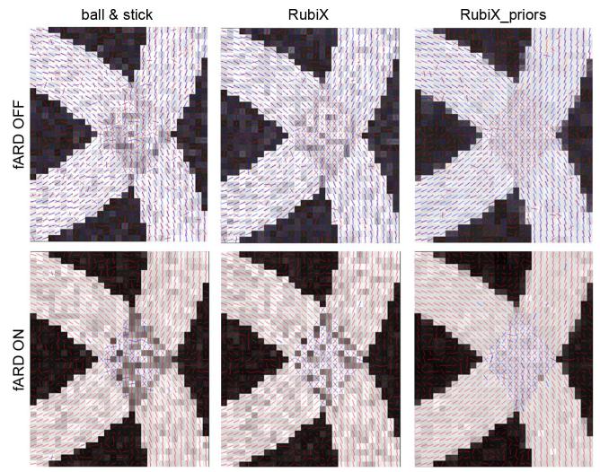
A simulated phantom with two crossing bundles (Fig. 2) was used to evaluate the performance of RubiX. The two bundles were embedded within isotropic background. The phantom included two slices with the elevation angle of the orientations being 0° for the first and 10° for the second slice (to aid visualization only the first slice is shown in Fig. 2). That ensured that orientations within 3D voxel neighborhoods were not replicated and were changing in all dimensions. Once the geometries were defined, data were obtained at two different spatial resolution grids (3 × 3 × 3 mm³ and mm 1.5 × 1.5 × 1.5 mm³) with a volume ratio V_LR = 8V_HR, so that each LR voxel contained 8 HR voxels. The signal at each HR voxel was simulated using the ball & stick model [12] with d = 0.001 mm/s² and total anisotropic volume fraction f s = ∑f = 0.6 (f₁ = f₂ = 0.3 at crossings) for the anisotropic regions. For the isotropic background, the signal from the ball compartment was used (f s = 0). The signal from groups of HR voxels was averaged to give the noise-free signal at a LR voxel. To simulate Rician noise, zero-mean Gaussian signal was added in quadrature. For a given SNR level Σ at high resolution, an SNR level of $8\Sigma ∕\sqrt{2}$ was used for the low resolution grid (see Appendix B).

Fig. 2.

Estimated fiber orientations for a simulated phantom using different methods (from left to right): the ball & stick model, the RubiX model and the RubiX model with conditional priors on the f s and d parameters. The phantom contains two curving bundles that cross, embedded within isotropic background. For each voxel, two orientations are estimated and the mode of the respective posterior distribution has been plotted. Orientation estimates are superimposed on the f s values, the total anisotropic volume fraction of each voxel. At the top row, only secondary orientations (colored in blue) with volume fraction f₂ > 5% are shown. For the results presented at the bottom row, an ARD prior has been applied to f₂, driving it to zero when a secondary fiber is not supported by the data. The SNR at the HR grid was 7.5 and b = 1000 s/mm² for both grids.

RubiX was compared against the ball & stick model applied on data generated at the high resolution grid. As each method considers different datasets, we matched their total acquisition time to make the comparisons fair. For single-shot diffusion EPI, the repetition time (TR) increases almost linearly with the number of slices. Assuming that we keep the field of view constant across resolutions and we increase slice thickness from HR to LR by a factor of $\mathcal{Z}$, we are able to acquire $\mathcal{Z}$ times more LR measurements in a given amount of time. If M_b measurements are considered for the ball & stick at the high resolution grid, we can parcellate the scanning time for RubiX, using M_HR and M_LR measurements, at HR and LR respectively, such that $M_{\mathrm{HR}}+M_{\mathrm{LR}}∕\mathcal{Z}=M_b$. In our specific example, where $\mathcal{Z}=2$, we used M_HR = M_LR = 120 and M_b = 180. Despite M_HR and M_LR being equal, the actual diffusion-sensitizing gradient directions were not the same for the two acquisitions.

Two sets of 174 and 114 directions were generated according to [29], so that any subset of the first M directions is isotropic. Six b = 0s/mm² measurement points were interspersed to each set, giving a total of 180 and 120 measurements. Data at the HR and LR were generated using the first and second set respectively. The ball & stick model was applied to the full HR dataset of 180 measurements, using the “bedpostX” toolbox [7] in FSL [30]. RubiX was applied to the first 120 HR measurements of the first set and the 120 LR measurements of the second set.

H. In Vivo MRI Data

A healthy male subject was scanned in a Siemens Trio 3T clinical imaging system. Two diffusion-weighted acquisitions (single-shot EPI) were performed at different spatial resolutions. For the HR acquisition, the acquisition matrix was 128×128 with in-plane resolution 1.5 × 1.5 mm² and 1.5 mm slice thickness (TE = 105 ms², TR = 11800 ms, 6/8 partial Fourier, FOV = 192 × 192 mm², 70 slices). Diffusion weighting was applied in 174 evenly spaced directions (generated as described in Simulations) with b = 1000 s/mm². For the LR acquisition, the FOV was kept the same, and the in-plane resolution was decreased to 3 × 3 mm² and 3 mm slice thickness (TE=86 ms, TR=4400 ms, 6/8 partial Fourier, FOV = 192 × 192 mm², 35 slices). Diffusion weighting was applied in 114 evenly spaced directions with b = 1000 s/mm². The bandwidth/pixel was kept the same for both acquisitions, so that distortions were of the same magnitude. Six volumes with no diffusion-weighting (b = 0 s/mm²) were acquired at each resolution, interspersed throughout the duration of the scans, giving a total of M_b = 180 and M_LR = 120 measurements.

We calculated the SNR of the b = 0 s/mm², for each of the two acquisitions. We used the two-ROI approach with the correction factors suggested in [31]. A tissue ROI was drawn in the midbody of the corpus callosum, where SNR measurements were performed. The LR and HR datasets had SNRs of roughly 50 and 8, respectively. The relative ratio is slightly higher than $8∕\sqrt{2}$ that has been used for the simulations, reflecting the effect of ignoring TE differences in the simulated datasets (i.e., simulation predictions reflect a more conservative scenario).

Each dataset was corrected for distortions using the following procedure. The susceptibility-induced distortions were corrected by acquiring extra data with reversed phase-encoding direction and applying the method of [32]. For each acquisition, the six b = 0 volumes were acquired twice with reversed phase-encoding directions. The susceptibility induced off-resonance field was calculated from these pairs. This field was fed into a Gaussian process predictor [33] that additionally estimated the eddy-current induced field and the subject movement for each volume of the dataset. The susceptibility induced field, the eddy current induced field and the subject movement was combined into a single transform for each volume and the resampling was performed using spline interpolation and Jacobian modulation. After distortion correction, the LR was registered to the HR dataset using a rigid body transformation and spline-based interpolation.

Similar to the simulations, the ball & stick model was applied to the full HR dataset of 180 measurements. RubiX was applied to the first 120 HR measurements of the full set and the 120 LR measurements. Notice that acquisition time was matched for both models. N = 2 fiber compartments were used for both models and L = 4 orientation prior modes for RubiX (unless otherwise stated). The MCMC samples were thinned by keeping one sample every forty. A burn-in MCMC period of 3000 and 5000 iterations was used for the ball & stick and RubiX, respectively. For RubiX, a longer burn-in period was utilized, as an order of magnitude more parameters are included in this model compared to the ball & stick. We tried burn-in periods of up to 50 000 iterations, with the results being identical.

III. Results

A. Simulations

A qualitative comparison of the ball & stick model with different versions of the RubiX model was first performed (Fig. 2). All models were applied to datasets that were matched for acquisition time. Specifically, the ball & stick model was applied to 180 measurements all at high-resolution. The RubiX models were applied to a combination of 120 measurements at HR and 120 measurements at LR. The simpler RubiX model includes only the conditional prior on the orientation parameters with L = 4 modes. The model denoted as RubiX_priors included also conditional priors on the anisotropic volume fraction f s and the diffusivity d. For all models, N = 2 fiber compartments were included. In Fig. 2, the modes of the posterior distribution of the orientations are plotted in each voxel. For the results presented at the bottom, ARD priors have been utilized on the volume fractions f, to enable “automatic” detection of crossing regions.

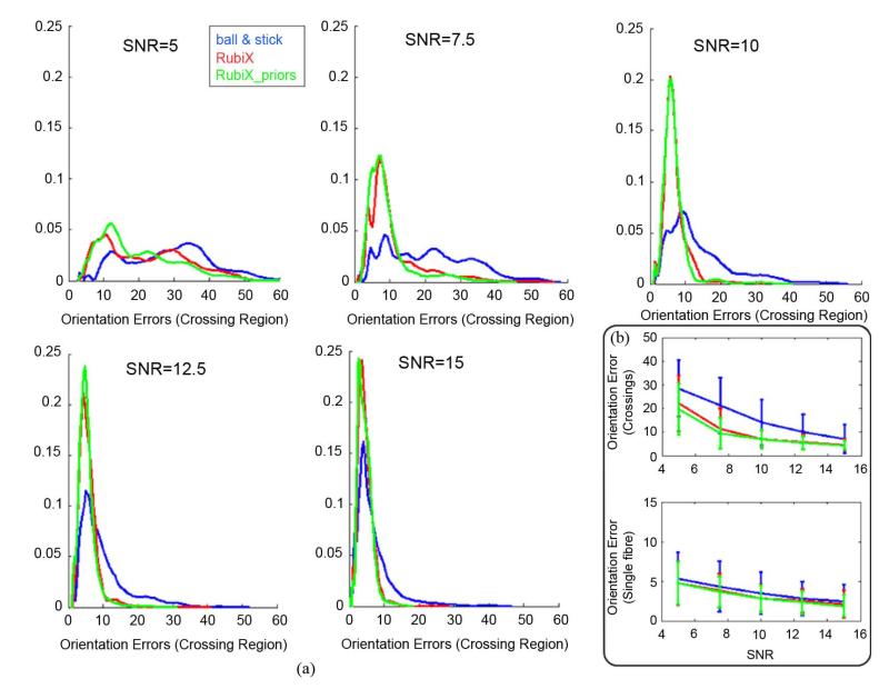
We can observe that the RubiX models always perform better in finding plausible and coherent orientations throughout the crossing. If the “automatic” crossing fiber detection is further desired (Fig. 2, bottom row), the inclusion of priors on the nuisance parameters f_s and d is beneficial in correctly identifying the crossing region. Figs. 3 and 4 quantify these improvements. Histograms of the orientation errors in the crossing region for the different models are shown in Fig. 3(a). For all SNR levels, RubiX performs clearly better, giving even at SNR = 7.5 a mean error of less than 10°. Interestingly, the ball & stick model exhibits a similar performance only for SNR = 12.5 (compare for instance the blue histogram at SNR = 12.5 to the green histogram at SNR = 7.5). This implies that, for this simulated example, the model that utilizes only the high spatial resolution data needs roughly three times more scanning time to achieve a similar performance as RubiX.

Fig. 3.

(a) Normalized histograms of orientation errors (in degrees) at the crossing region of the phantom. The fiber orientations estimated using different methods (ARD for volume fractions is off) are compared to the ground truth orientations for different SNR levels. SNR is of the HR grid. (b) Errorbars showing the mean (±standard deviation) of orientation errors at the crossing and the single-fiber region of the phantom, as a function of the HR SNR. b = 1000 s/mm² was used for both grids of the RubiX dataset.

Fig. 4.

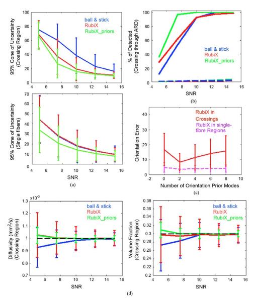
(a) Cones of uncertainty (95%) of the estimated orientations at the crossing and single-fiber region of the phantom, using different methods, as a function of the HR SNR. Vertical axis is in degrees. (b) Effectiveness of the ARD prior on the volume fractions to detect crossings. Solid lines correspond to the % of correctly resolved crossings. Dashed lines correspond to false positives, crossings identified in the single-fiber region. (c) The effect of the number of modes L of the RubiX conditional prior on the orientations. Errorbars indicate the mean (±standard deviation) orientation error (in degrees). SNR of the HR data was 7.5. (d) Diffusivity and volume fraction estimates at the crossing region, as a function of the HR SNR. Errorbars represent the mean (±standard deviation) of the estimates. For the volume fraction values, the mean of f₁ and f₂ in the crossing region is reported. The ground-truth values are depicted by the dashed black lines.

Fig. 3(b) summarizes the histogram information by presenting errorbars (mean error ± st. dev.) for the crossing and single-fiber regions. RubiX is superior in all cases, but the benefit in using it is particularly evident at the crossing.

Other aspects of the RubiX performance are quantified in Fig. 4. Panel (a) shows errorbar plots of the 95% cones of orientational uncertainty [34]. These are representative of how wide the estimated orientation distributions are. RubiX again performs better in reducing the uncertainty, giving more precise estimates than the ball & stick model. Panels (a) and (b) further illustrate the effect of the conditional priors on the nuisance parameters. The orientational uncertainty becomes smaller when these priors are included into the RubiX model (red versus green curves). More importantly, however, they seem beneficial for the performance of the automatic crossing detection through the ARD priors. Panel (b) shows the improved sensitivity of RubiX when these priors are employed, allowing an almost 100% detection of crossing voxels, even at an SNR of 7.5 (see also Fig. 2). This improvement is not against specificity. Even if there is a slight increase of false positives (dashed lines) with RubiX_priors, these are kept at very low levels (< 3%) for all models. Even in the cases, though, where multiple fiber compartments are identified in single-fiber regions, these mostly have an orientation commensurate to the ground truth.

For the RubiX simulations so far, we have fixed the number of modes of the orientation prior L = 4. Why in the first place do we need such a prior? In the event of very noisy HR data, orientation patterns cannot be localized within each HR voxel using the LR data alone. The orientation prior imposes a constraint on the solution space, by requiring a priori that the estimated HR orientations are close to the modes of this prior [see Fig. 1(b)]. This constraint is driven by the data, as both the modes and the dispersion around them are estimated during the model inversion (even if small dispersion values are encouraged by the respective hyper-prior). In general, we expect that the modes of the prior reflect the predominant orientations in an LR voxel. The number of modes effectively determines how strict such a prior constraint is. For instance, by using one mode, we a priori require that all estimated orientations are concentrated around this mode. More modes give less spatial regularization constraints, but also more hyper-parameters to estimate from the data. In Fig. 4(c), we illustrate the effect of changing the number of modes L, from zero to eight, on the orientation errors. For two modes we get the smallest errors, which increase with L. For the extreme case of L = 8, the performance is very similar to the case with L = 0, reflecting the difficulty of the model to infer so many parameters from the data. We chose L = 4 as a good compromise between estimation accuracy and softness of the constraint.

We should point out that the orientation prior is not necessary to obtain improvements over the ball & stick estimates. The mean orientation error in the crossing region for RubiX with 0 modes (i.e., no orientation prior) is 16.75°, while for the ball & stick model 21.25°. However, the utilization of such a prior gives more accurate and precise estimates [Fig. 4(c)].

We examined the accuracy of RubiX in estimating model parameters other than the orientations. Fig. 4(d) shows the performance of all methods in resolving the diffusivity d and the volume fractions f in the more complex crossing region. As expected, the RubiX estimates are more accurate on average, with the inclusion of the conditional priors on the nuisance parameters increasing the precision, as well.

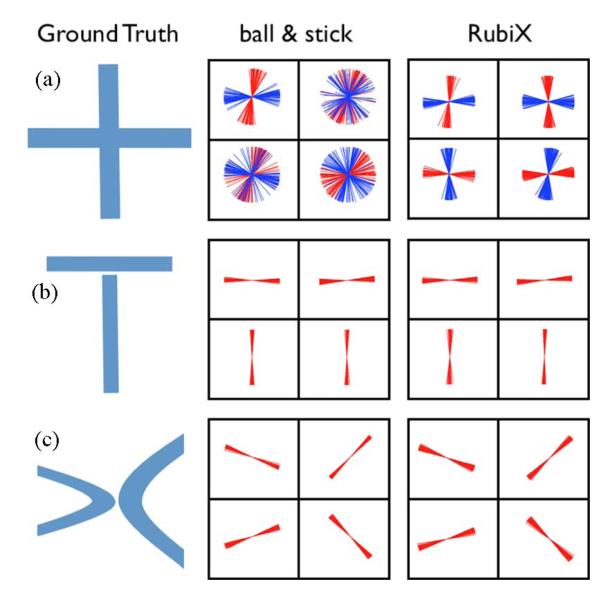
Apart from the increased sensitivity in detecting crossings, due to the enhanced SNR of the low-resolution grid, RubiX should in principle benefit from the spatial specificity offered by the high-resolution grid. We therefore examined whether it offers similar localization performance compared to a method that performs directly on the HR grid. To test that, we simulated complex fiber patterns that all result in an apparent “crossing” profile when imaged at low resolution (Fig. 5); an orthogonal crossing (a), a “sandwich” crossing (b), and a “kissing” fiber scenario (c). Notice that the LR signal obtained from patterns (a) and (b) would be exactly the same. RubiX utilizes the extra SNR to robustly resolve the fiber crossing in (a), much better than the ball & stick model that uses more (but noisy) HR data. At the same time, it performs equally well in localizing the tracts in cases (b) and (c), without estimating fictitious crossings (as would be suggested by the LR data alone).

Fig. 5.

Localization of different fiber configurations using RubiX. (a) Orthogonal crossing. (b) “Sandwich” crossing. (c) Fiber kissing. In each voxel, samples from the posterior distribution of the orientations have been plotted to illustrate the uncertainty associated with each estimated orientation. Notice that (a) and (b) will give the same LR data. The SNR of the HR data was 7.5 and b = 1000 s/mm² for both resolutions. An ARD prior has been applied to f₂, for automatically detecting fiber crossings.

B. In Vivo Data

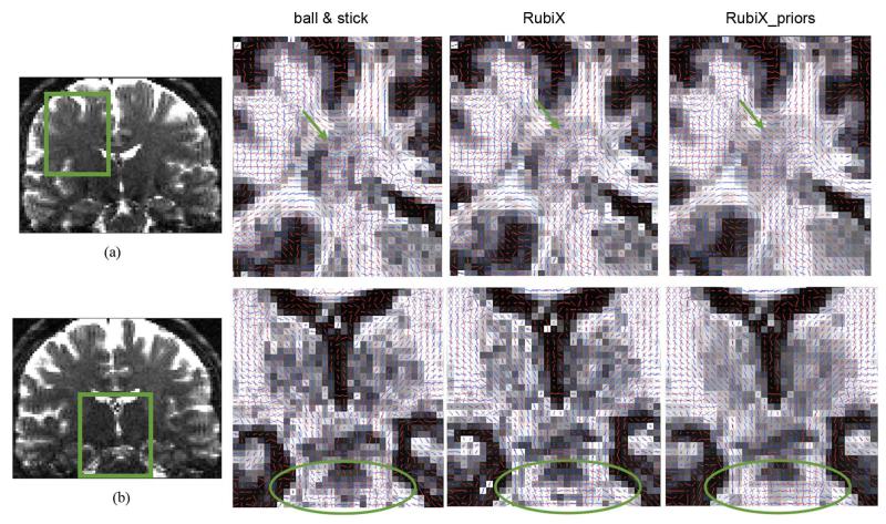
Similar to simulations, RubiX was applied to HR and LR data (120 measurements for each resolution) and was compared against the ball & stick model applied to the full HR dataset (180 measurements). Fig. 6 presents the mean estimated orientations of two fiber compartments for different models. The ARD prior on the volume fractions was turned off for all models, in order to illustrate the effect of RubiX on the estimated orientations alone. A second orientation is shown only for voxels with f₂ > 5%.

Fig. 6.

Coronal views of mean estimated orientations of two fiber compartments for different models (from left to right): The ball & stick model, the RubiX model with orientation conditional priors and the RubiX model with orientation, volume fraction (f_s) and diffusivity (d) conditional priors. (a) Area close to the centrum semiovale (green arrow). (b) Region around the orthogonal crossing between the corticospinal tract and the transverse pontine fibers (shown encircled). The orientation vectors are superimposed on the f_s maps, estimated by each method. A second orientation vector is shown in blue only for voxels where f₂ > 5%.

Fig. 6(a) shows a coronal perspective of an area around the centrum semiovale (green arrow). We can observe that the ball & stick estimates are relatively noisy in recovering the crossing of bundles in the pyramidal tract (mostly superior-inferior orientation) and in the callosal tracts (mostly medial-lateral orientation). Both versions of RubiX are more successful in reconstructing a coherent crossing, with the inclusion of priors on the nuisance parameters being beneficial. RubiX estimates seem better in other areas, as well. The crossings at the internal capsule between the pyramidal tract and thalamocortical projections or the external capsule are much noiser with the ball & stick model.

A similar picture is illustrated in Fig. 6(b), at the crossing between the transverse pontine fibers and the corticospinal tract (shown encircled). RubiX models resolve much better this orthogonal crossing, with the estimates clearly suggesting the orientations of the two bundles.

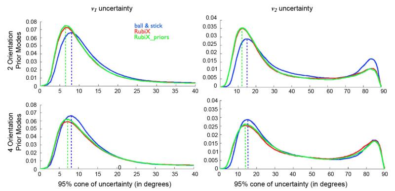
Apart from the increased spatial coherence, precision of the RubiX estimates is also improved compared to the ball & stick model. Fig. 7 shows histograms of the 95% cones of orientation uncertainty across all white matter voxels. A white matter mask was obtained using an automatic segmentation of a T1-weighted anatomical scan (“Fast” toolbox in FSL) [35]. Such a mask is not perfect and in our case contained subcortical gray matter regions. Therefore, we further performed a mask erosion to exclude such regions and white/gray matter interfaces. Focusing on the core of white matter, histograms for the principal fiber orientation v₁ appear unimodal. For the secondary fiber orientation v₂, the histograms are bimodal, with the second peak representing white matter voxels where a second fiber is not strongly supported by the data.

Fig. 7.

Normalized histograms of 95% cones of orientation uncertainty in white matter, using different models. Voxels have been selected using an eroded WM mask, segmented from a T1-weighted anatomical scan. The two columns correspond to uncertainty on the principle v₁ and secondary v₂ fiber orientation, respectively. Each row corresponds to different RubiX models with different number L of orientation prior modes. No ARD priors were used for the volume fractions. The dashed lines aid visualization and illustrate the values at which each histogram attains its first peak.

Fig. 7 shows how the uncertainty changes with different models and different numbers of orientation prior modes L in the RubiX model. For all cases, RubiX histograms attain their peak at a smaller value, suggesting that the estimated orientation uncertainty is smaller in white matter. When L = 2 modes are used the mean WM uncertainty in v₁ and v₂ drops by 22% and 19% for RubiX compared to the ball & stick model. For L = 4, the decrease is of the order of 11% and 9%. Furthermore, for L = 2, RubiX found more WM voxels having lower uncertainty on the secondary orientation, suggesting more crossings detected more precisely. However, this is not the case for L = 4, suggesting that this in vivo dataset does not strongly support as many modes in the orientation prior.

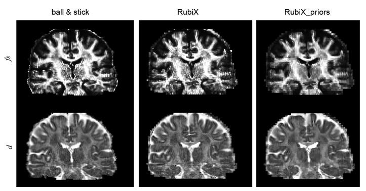
Figs. 8 and 9 present RubiX estimates for other parameters of the model. Fig. 8 shows maps of the total anisotropic volume fraction f s and the diffusivity d. As we can observe, the incorporation of the conditional priors on the nuisance parameters f s and d, lead to smoother spatial maps, as expected. However, edges are preserved. In Fig. 9, we present maps of the estimated hyperparameters f s_m, d_m, and μ₁. These correspond to modes of the different conditional priors and are estimated at the LR grid. Notice that these maps are used to a priori constrain the respective HR parameters, for instance f s and d shown in the last column of Fig. 8.

Fig. 8.

Maps of anisotropic volume fractions and diffusivities estimated using different models. Including the conditional priors on the nuisance parameters f s and d in RubiX leads to edge-preserving spatial smoothing. At each voxel, the mean of the respective estimated posterior distribution has been plotted.

Fig. 9.

Estimated hyper-parameters from RubiX, when conditional priors are utilized in the model. From left to right: mean of the Normal prior imposed on the sum of anisotropic volume fractions, mean of the Normal prior imposed on the diffusivities and one of the modes of the orientation prior. As these parameters influence the group of HR voxels that are intersected by each LR voxel, they are estimated at the low-resolution grid. Notice that a posterior distribution for each of these parameters is estimated. The maps present the means of these distributions. For μ₁, the mean dyadic vector is plotted, RGB color-coded and modulated by the corresponding f s_m value.

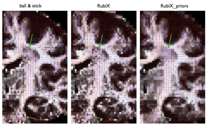
We further tested the performance of RubiX models, when the “automatic” crossing detection is turned on, using the ARD priors on the volume fractions f₂. Fig. 10 illustrates a coronal perspective of the mean orientations estimated through different models. As expected from the results on the simulated phantom, the conditional prior on the nuisance parameters f s and d is beneficial for increasing the number of detected crossings (last column of Fig. 10). A few crossing examples are indicated by the green arrows, at the centrum semiovale and the pons.

Fig. 10.

Coronal views of mean estimated orientations of two fiber compartments for different models (from left to right): The ball & stick model, the RubiX model with orientation conditional priors and the RubiX model with orientation, volume fraction (f s) and diffusivity (d) conditional priors. For all models an ARD prior was employed for f₂. The orientation vectors are superimposed on the f s maps, estimated by each method. A second orientation vector is shown in blue only for voxels where f₂ > 0.05.

C. Spatial Specificity of Rubix Estimates

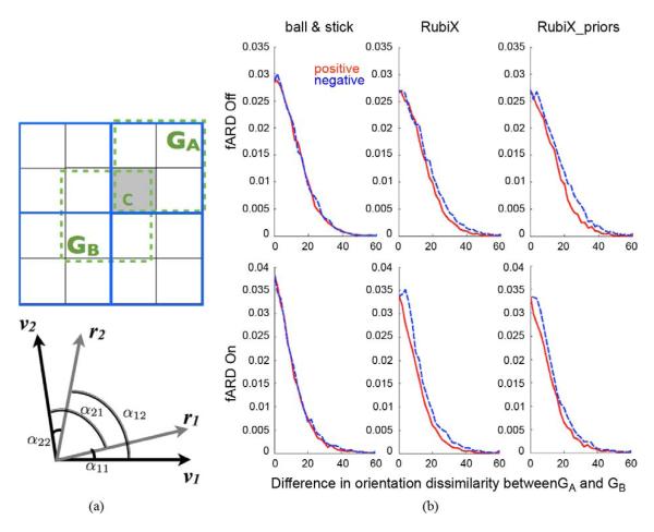
So far, we have illustrated the benefits gained from the multi-resolution RubiX approach. However a fundamental question remains to be explored. Even if RubiX model parameters are estimated at the highest of the spatial resolutions, do we recover the spatial specificity offered by such a HR grid? Or are the estimates somewhat biased by the lower resolution measurements? To examine this, we explored how orientation estimates change within different subgroups of HR voxels. As shown in Fig. 11(a), we considered a first subgroup G_A consisting of HR voxels intersected by the same LR voxel. When running RubiX, the estimates at these voxels are obtained using the same model fit. We further considered a second subgroup G_B that consists of HR voxels intersected by different LR voxels (there are eight such subgroups in our example). The estimates at these voxels are obtained by eight independent RubiX model fits. In the presence of biases, we expect that the orientation similarity in G_A is consistently larger than the similarity in G_B (or that the orientation dissimilarity in G_A is smaller than in G_B).

Fig. 11.

(a) Top: Subgroups of HR voxels used to assess orientation dissimilarity. The high-resolution grid is depicted using the black lines, while the low-resolution grid is shown in blue. For a voxel c, we define G_A, containing all the HR voxels intersected by the same LR one and G_B that contains neighboring HR voxels, intersected by different LR voxels. Bottom: Angles used to assess dissimilarity between the two orientation estimates of two voxels. (b) Normalized histograms of orientation dissimilarity differences (in degrees) between subgroups G_A and G_B. To aid visualization, positive differences are shown in red and the absolute values of the negative differences are shown in blue. Differences are computed across WM.

We utilized the white matter orientation estimates from a whole-brain RubiX analysis to explore this issue. Given that two orientations are estimated in each voxel, we assessed the dissimilarity between two voxels, by considering the angles illustrated at the bottom of Fig. 11(a). If v₁, v₂, and r₁, r₂ are respectively the mean orientation estimates of the two voxels, we calculated the dissimilarity Δ, considering in each voxel only the orientations with a volume fraction f > 5%. If two orientations were supported for both voxels, then the dissimilarity was Δ = min(β₁, β₂), with β₁ = max(α₁₁, α₂₂) and β₂ = max(α₁₂, α₂₁). If one of the voxels had only one orientation supported, then Δ = min(α₁₁, α₁₂). For all other cases Δ = α₁₁. Then, for a voxel c within a subgroup G, the dissimilarity ${\Delta }_G^c$ was the mean of the dissimilarities of c with all the other voxels in G. For each voxel in white matter, we computed the difference between the dissimilarities ${\Delta }_{G_A}^c$ and ${\Delta }_{G_B}^c$. Fig. 11(b) shows histograms of these differences for different models. To aid visualization and assess the symmetricity of the histograms, we present the positive differences (red lines) and the absolute value of the negative differences (blue dashed lines). In the absence of any bias, we expect that the red and blue lines overlap.

As we can observe, the histograms appear almost perfectly symmetric for the ball & stick model, which operates directly on the high resolution dataset. For RubiX models, we can observe some asymmetry, with the negative branch of the histogram being slightly wider. This suggests that the orientation dissimilarity in subgroups G_B is consistently higher than the one in subgroups G_A. However, for the cases where ARD is off (top histograms) and where ARD is on (bottom histograms), the bias is in the order of 1.5 and 2 degrees on average.

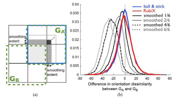
From these results, RubiX estimates appear to have less spatial specificity than the one offered by the high resolution grid. What spatial specificity then does RubiX recover? To answer this, we compared the orientation dissimilarity histograms of RubiX (as shown in Fig. 11) with respective histograms from the ball & stick model fitted to smoothed versions of the HR data. Smoothing was confined within the subgroups G_A of HR voxels [Fig. 11(a)], by setting the signal at each voxel equal to a weighted average of the signal of the voxels within the subgroup. Weights were defined according to the chosen smoothing extent. As shown in Fig. 12(a), the smoothing extent (which was kept the same for all dimensions) defined the contribution of the neighbors. The relative volumes of the gray-shaded regions determined the weights. A large smoothing extent results to larger weights and thus more spatial smoothing. We considered six smoothing extents (1/6 to 6/6—fractions of the voxel dimensions), with 6/6 meaning equal weights for all neighbors (i.e., signal at each voxel was simply the arithmetic mean of the signals within the subgroup). For each smoothed dataset, orientations were estimated using the ball & stick model.

Fig. 12.

(a) Spatial smoothing was performed within subgroups G_A of HR voxels, intersected by the same LR voxel. The smoothing was performed using a weighted average of the signals within the subgroup, with the weights for each voxel defined by the smoothing extent. The smoothing extent (fraction of the voxel dimensions) defined the contributions of the neighbors and the weights were proportional to the relative volumes of the contributed (gray-shaded) regions. (b) Normalized histograms of orientation dissimilarity differences (in degrees) between subgroups G_A and G_B. Red corresponds to RubiX estimates and blue to ball & stick. The histograms depicted by black and gray colors correspond to ball & stick estimates from smoothed datasets. Dissimilarity differences are computed across WM. All models had an ARD prior for f₂. For RubiX, the priors on the nuisance parameters (f_s, d) were also utilized.

Fig. 12(b) shows that the RubiX histogram (red) is slightly less symmetric and with fatter tails than the ball & stick one (blue); however, it is much more symmetric than any of the smoothed datasets. Even a smoothing extent of 1/6 (0.25 mm) introduces twice as much bias, on average. These results verify that although the spatial specificity of RubiX estimates is not exactly the one offered by the high resolution grid, it is extremely close to.

D. Accuracy of In Vivo Orientation Estimates

RubiX has been shown in simulations to improve accuracy of orientation estimates compared to the ball & stick model. To assess accuracy of in vivo estimates, a ground-truth high-resolution dataset is needed. This would, however, require very long acquisition times. Therefore, we performed a cross-validation test to address this question.

The full 180 measurement, high-resolution dataset was divided into two datasets, one with 120 and one with 60 measurements. We ran the ball & stick model on these datasets and used the estimates from the 120-measurement one as “ground-truth.” The accuracy of the 60-measurement ball & stick estimates was then compared to the accuracy of the RubiX estimates obtained from 40 HR (subset of these 60) and 40 LR measurements (i.e., ball & stick and RubiX datasets were matched for acquisition time). Note that whilst the 120-measurement dataset is a very noisy estimate of ground truth, these data are a result of twice the acquisition time as the 60-measurement ball & stick or the RubiX analyses. Note also that, given the “ground truth,” the ball & stick model starts this comparison with an advantage. First, the same model is used to get the ground-truth estimates. Second, we have shown that RubiX (Fig. 12) does not fully recover the spatial specificity of the high-resolution grid. Therefore, the ground truth for RubiX should be orientation estimates at a slightly lower spatial resolution.

Despite these disadvantages, the RubiX estimates agree more on average with the “ground-truth” estimates than the ball & stick ones. For an ROI that included the bilateral crossing between the corpus callosum and the superior longitudinal fasciculus, within the centrum semiovale, the mean orientation error was 12.81 for RubiX and 15.64 for the ball & stick model. Furthermore, RubiX identified 74% of the voxels that contained a crossing, according to the “ground-truth.” The ball & stick model identified 61% of the crossing voxels.

IV. Discussion

We have presented a model that simultaneously considers diffusion-weighted MRI data acquired at multiple spatial resolutions to infer fiber orientations. RubiX combines the spatial specificity and SNR benefits of the high and low-resolution grids, respectively, to estimate more robustly orientations at the highest of the available resolutions. In simulations and in vivo human brain data, RubiX has been shown to estimate crossing patterns more accurately and with less uncertainty compared to a model that utilizes only high-resolution data, matched for acquisition time with the multi-resolution protocol. For the in vivo data, RubiX estimates agree more with our prior anatomical knowledge for regions such as the centrum semiovale and the pons. The current study illustrates the value of spending some of the acquisition time for collecting data at a lower (than desired) spatial resolution, rather than collecting more, but noisier data only at high resolution.

The RubiX framework combines a local model for predicting the signal at the HR grid and a partial volume model for making LR predictions. Conditional priors are also utilized on some of the parameters (orientations, volume fractions and diffusivity). The priors reduce identifiability issues, when the high resolution data have very poor SNR, at the expense of some spatial regularization. Priors on the nuisance parameters f s and d, in particular, assist the selection of the supported-by-the-data complexity through the ARD (Fig. 2, Fig. 4(b), and Fig. 10). As shown in the results, they are not essential for improving performance compared to the single-resolution, ball & stick model, but they do increase robustness and spatial coherence. This is particularly true for the orientation prior, as shown in Fig. 4(c). RubiX estimates without any orientation prior (0 modes) are more accurate than the ball & stick estimates [Fig. 3(b)]. However, the prior improves significantly both accuracy and precision in this simple simulation.

An important feature of all these priors is that they are specified by hyper-parameters of the model, which are directly estimated from the data. As the hyper-parameters are common to subgroups of HR voxels, intersected by a single LR voxel, their values are mostly influenced by the way fiber patterns are depicted at LR. At the same time, they act as constraints on the parameters defined on the HR grid [Fig. 1(b)].

Attempts have been recently made for reconstructing high-resolution (HR) DWI, by combining a set of low-resolution (LR) images. In [36], the authors proposed a method for super-resolution DWI using multiple anisotropic and orthogonal LR acquisitions. The reconstruction was based on a generative model of the acquired low-resolution volumes from the unknown high-resolution ones to be estimated. A similar approach was recently presented in [37], but the combined LR volumes could have arbitrary slice-encoding directions (not necessarily orthogonal). As before, the proposed model resolved a HR volume for a specific diffusion-sensitizing gradient from a set of a LR acquisitions of the same gradient orientation. Following a different perspective, [38] produced very high spatial resolution images of track density (TD), using the reconstructed curves of white matter tractography. Even if the resolution of the acquired data is not changed, utilizing the spatial information encoded by the tractography curves results in postprocessed, increased-resolution TD images. The method effectively performed a rebinning of the spatial distribution of curves into a finer scale.

All these super-resolution approaches utilize LR acquisitions and attempt to enhance the spatial resolution. Our proposed framework is different in spirit and aim. We actually combine both high and low spatial resolutions into a single data-fusion analysis to estimate microstructural features at the highest of the available resolutions. An alternative to our Bayesian approach might use scale-space theory [39]–[41] on the image space or k-space directly. Bayesian theory, however, allowed more flexibility in our context as well as direct uncertainty quantification of the model parameter estimates.

Given the fusion of LR and HR data, a natural question arises on the spatial specificity of the RubiX estimates; even if the parameters of interest are defined on the high-resolution grid. Simple simulations illustrated the localization features of RubiX and the ability of the model to estimate robustly different fiber patterns that are described by similar LR data (Fig. 5). We also performed extensive tests to address this question using in vivo data (Figs. 11, 12). We found that the spatial specificity of RubiX estimates is not exactly the one of the high resolution grid, as there is a small bias of increased similarity introduced within subgroups of HR voxels. However, it is very close to the HR spatial specificity. Smoothing of the HR data with extents as small as 1/6 of the voxel dimensions introduces twice as much bias.

For the RubiX analyses presented in this study, we utilized the same number of measurements at each spatial resolution. Too few datapoints at the high resolution will impose identifiability issues and reduce the spatial specificity of the estimates. On the other hand, too few datapoints at the low resolution will hardly offer any advantage compared to a single-resolution method. We chose a middle-ground solution for this trade-off, but clearly an optimized parcellation of the data acquisition time requires a separate study.

The current local model (Section II-A) is of mono-exponential decay in q-space and is used to make predictions for both LR and HR measurements. Therefore, it is only valid for cases where the b value is kept the same for both spatial resolutions. In our in vivo dataset the b value was kept low (1000 s/mm²). As an increase in both the value and the spatial resolution will dramatically reduce the SNR, a better choice for a multi-resolution protocol would be to scan at a low b value and high spatial resolution and at a high b value and low spatial resolution. Such protocols cannot be accommodated by the current local model. However, the model recently introduced by [22] could be used instead. Such a model assumes a continuous distribution of diffusivities, therefore exhibiting multi-exponential decay. We anticipate that such an extension will increase sensitivity particularly to three-way crossings. With the current low-b dataset, RubiX significantly decreased noise artifacts compared to the ball & stick model, when both ran with N = 3, but utilizing the volume fraction ARD priors allowed only very few third fibers to be strongly supported by the data.

Another assumption of the current local model is that the apparent diffusivity remains relatively constant for the different echo times (TE) employed in the two combined acquisitions. Even if a change in diffusivity is theoretically expected with a change in TE, this has been shown to be in the order of 1%–2% [42] for the TEs employed here, making the above assumption reasonable. Notice that the local model of [22] discussed above could remedy this issue as well, when TE differences are larger.

The local models mentioned so far can capture within-voxel crossing patterns. Resolving fiber crossings is important for tractography [7], but more complicated fiber patterns still pose problems to tracking algorithms [3]. Therefore, other local models that capture more complex fiber patterns can be utilized within RubiX, such as models that capture within-voxel fiber dispersion [8], [43]. Such models are more sensitive to noise and are expected to benefit from the multi-resolution framework. Furthermore, it should be noted that the local model used in this study may not be appropriate for gray matter, as recently showed in [43]. The estimated diffusivities and volume fractions, particularly, may be much less accurate compared to respective estimates in white matter.

A limitation of the current RubiX implementation is the utilization of a Gaussian noise model. This will reduce the accuracy of the estimates, particularly in cases of very low SNR at the highest of the resolutions. Incorporation of a Rician noise model would, however, be straightforward within the presented framework. Accuracy is expected to increase in the expense of increased computation time. However, we do not expect the effects on the performance from such a change to be dramatic, as shown by our simulations (where Rician noise was added to the data).

Another requirement of the current RubiX implementation is that the spatial resolution grids have integer volume fractions. This allowed a relatively simple MCMC implementation. Model fits in subgroups of few voxels could be performed independently allowing faster MCMC convergence, and also faster computation through parallelization (approximately 9 h on 30 nodes of a CPU cluster for a subject). An implementation that would permit arbitrary spatial resolutions to be combined could simply follow the same principles and models. However, it would make parallelization challenging and was therefore out of the scope of this study.

Appendix A. Integrating Out Noise Parameters

The likelihood function described in (4) depends on P_LR and P_HR terms. For each of these terms, the parameters σ_LR and σ_HR can be integrated out respectively. Assume the precision parameters τ = 1/σ², instead, and reference priors P(τ) = 1/τ. These priors have the smallest possible influence on the posterior distribution [44]. Then

$$P_{\mathrm{LR}}({\mathbf{Y}}_{\mathrm{LR}}\mid \Omega )={\int }_0^{\infty }{P}_{\mathrm{LR}}({\mathbf{Y}}_{\mathrm{LR}}\mid \Omega ,{\tau }_{\mathrm{LR}})P\left({\tau }_{\mathrm{LR}}\right)d{\tau }_{\mathrm{LR}}.$$ (12)

Substituting above with a multivariate Normal and the reference prior and using the identity ${\int }_0^{\infty }{t}^{a-1}{e}^{-\mathit{bt}}\mathit{dt}=\Gamma \left(a\right)∕b^a$, we get

$$P_{\mathrm{LR}}({\mathbf{Y}}_{\mathrm{LR}}\mid {\Omega }^{\prime })\propto {\left[\frac{1}{2}\sum _{M=1}^{M_{\mathrm{LR}}}{\left(y_{\mathrm{LR}}^M-S_{\mathrm{LR}}^M\right)}^2\right]}^{-M_{\mathrm{LR}}∕2}$$ (13)

where the parameter space Ω′ = Ω − {σ}. Similarly for Y_HR

$$P_{\mathrm{HR}}({\mathbf{Y}}_{\mathrm{HR}}^k\mid {\Omega }^{\prime })\propto {\left[\frac{1}{2}\sum _{m=1}^{M_{\mathrm{HR}}}{\left(y_{\mathrm{HR}}^{\mathit{km}}-S_{\mathrm{HR}}^{\mathit{km}}\right)}^2\right]}^{-M_{\mathrm{HR}}∕2}.$$ (14)

Appendix B. SNR at Different Spatial Resolutions

The signal to noise ratio decreases as spatial resolution increases. According to [5], for a general 3-D acquisition

$$\mathrm{SNR}\propto V\sqrt{\frac{N_x{N}_y{N}_z}{{\mathit{BW}}_{\text{read}}}}$$ (15)

with V being the voxel volume, N_i the number of k-space measurements in direction i and BW_read is the bandwidth in the readout direction.

For a 2-D acquisition, as in diffusion EPI, this can be rewritten as

$$\mathrm{SNR}\propto V\sqrt{\frac{N_x{N}_y}{{\mathit{BW}}_{\text{read}}}}=V\sqrt{\frac{N_x{N}_y}{N_x{\mathit{BW}}_{\text{pixel}}}}=V\sqrt{\frac{N_y}{{\mathit{BW}}_{\text{pixel}}}}$$ (16)

with BW_pixel the bandwidth per pixel. When the spatial resolution increases by keeping a constant field of view and increasing the matrix size, the SNR change will depend on the change in V and N_y (assuming that BW_pixel, and thus distortions, are kept constant). For instance, increasing the spatial resolution from 3 × 3 × 3 mm³ to 1.5 × 1.5 × 1.5 mm³ by doubling the matrix size in each dimension will cause an SNR drop of $8∕\sqrt{2}$.

References

- [1].Mori S, Crain BJ, Chacko VP, van Zijl PC. Three-dimensional tracking of axonal projections in the brain by magnetic resonance imaging. Ann. Neurol. 1999;vol. 45:265–9. doi: 10.1002/1531-8249(199902)45:2<265::aid-ana21>3.0.co;2-3. [DOI] [PubMed] [Google Scholar]
- [2].Basser PJ, Pajevic S, Pierpaoli C, Duda J, Aldroubi A. In vivo fiber tractography using DT-MRI data. Magn. Reson. Med. 2000;vol. 44(no. 4):625–32. doi: 10.1002/1522-2594(200010)44:4<625::aid-mrm17>3.0.co;2-o. [DOI] [PubMed] [Google Scholar]
- [3].Jbabdi S, Johansen-Berg H. Tractography: Where do we go from here? Brain Connect. 2011;vol. 1(no. 3):169–183. doi: 10.1089/brain.2011.0033. [DOI] [PMC free article] [PubMed] [Google Scholar]
- [4].Seunarine KK, Alexander DC. Multiple fibers: Beyond the diffusion tensor. In: Johansen-Berg H, Behrens T, editors. Diffusion MRI: From Quantitative Measurement to in vivo Neuroanatomy. Elsevier; New York: 2009. pp. 55–72. [Google Scholar]
- [5].Haacke EM, Brown RW, Thompson MR, Venkatesan R. Magnetic Resonance Imaging: Physical Principles and Sequence Design. Wiley; New York: 1999. [Google Scholar]
- [6].Tournier JD, Calamante F, Gadian DG, Connelly A. Direct estimation of the fiber orientation density function from diffusion-weighted MRI data using spherical deconvolution. Neuroimage. 2004;vol. 23:1176–85. doi: 10.1016/j.neuroimage.2004.07.037. [DOI] [PubMed] [Google Scholar]
- [7].Behrens TE, Berg HJ, Jbabdi S, Rushworth MF, Woolrich MW. Probabilistic diffusion tractography with multiple fibre orientations: What can we gain? Neuroimage. 2007;vol. 34(no. 1):144–55. doi: 10.1016/j.neuroimage.2006.09.018. [DOI] [PMC free article] [PubMed] [Google Scholar]
- [8].Sotiropoulos SN, Behrens TEJ, Jbabdi S. Ball and rackets: Inferring fiber fanning from diffusion-weighted MRI. NeuroImage. 2012;vol. 60(no. 2):1412–1425. doi: 10.1016/j.neuroimage.2012.01.056. [DOI] [PMC free article] [PubMed] [Google Scholar]
- [9].Jeurissen B, Leemans A, Tournier JD, Jones DK, Sijbers J. Investigating the prevalence of complex fiber configurations in white matter tissue with diffusion magnetic resonance imaging. Human Brain Mapp. 2012 doi: 10.1002/hbm.22099. [DOI] [PMC free article] [PubMed] [Google Scholar]
- [10].Miller K, Stagg C, Douaud G, Jbabdi S, Smith S, Behrens T, Jenkinson M, Chance S, Esiri M, Voets N, Jenkinson N, Aziz T, Turner M, Johansen-Berg H, McNab J. Diffusion imaging of whole, post-mortem human brains on a clinical MRI scanner. NeuroImage. 2011;vol. 57:167–181. doi: 10.1016/j.neuroimage.2011.03.070. [DOI] [PMC free article] [PubMed] [Google Scholar]
- [11].Tuch DS, Reese TG, Wiegell MR, Makris N, Belliveau JW, Wedeen VJ. High angular resolution diffusion imaging reveals intravoxel white matter fiber heterogeneity. Magn. Reson. Med. 2002;vol. 48:577–82. doi: 10.1002/mrm.10268. [DOI] [PubMed] [Google Scholar]
- [12].Behrens TE, Woolrich MW, Jenkinson M, Johansen-Berg H, Nunes RG, Clare S, Matthews PM, Brady JM, Smith SM. Characterization and propagation of uncertainty in diffusion-weighted MR imaging. Magn. Reson. Med. 2003;vol. 50(no. 5):1077–88. doi: 10.1002/mrm.10609. [DOI] [PubMed] [Google Scholar]
- [13].Kaden E, Knosche TR, Anwander A. Parametric spherical deconvolution: Inferring anatomical connectivity using diffusion MR imaging. Neuroimage. 2007;vol. 37(no. 2):474–488. doi: 10.1016/j.neuroimage.2007.05.012. [DOI] [PubMed] [Google Scholar]
- [14].Sotiropoulos SN, Bai L, Morgan PS, Auer DP, Constantinescu CS, Tench CR. A regularized two-tensor model fit to low angular resolution diffusion images using basis directions. J. Magn. Reson. Imag. 2008;vol. 28:199–209. doi: 10.1002/jmri.21380. [DOI] [PubMed] [Google Scholar]
- [15].Tuch DS. Q-ball imaging. Magn. Reson. Med. 2004;vol. 52:1358–72. doi: 10.1002/mrm.20279. [DOI] [PubMed] [Google Scholar]
- [16].Jansons KM, Alexander DC. Persistent angular structure: New insights from diffusion magnetic resonance imaging data. Inverse Problems. 2003;vol. 19:1031–1046. [Google Scholar]
- [17].Ozarslan E, Shepherd TM, Vemuri BC, Blackband SJ, Mareci TH. Resolution of complex tissue microarchitecture using the diffusion orientation transform (DOT) Neuroimage. 2006;vol. 31:1086–103. doi: 10.1016/j.neuroimage.2006.01.024. [DOI] [PubMed] [Google Scholar]
- [18].Descoteaux M, Angelino E, Fitzgibbons S, Deriche R. Regularized, fast, and robust analytical Q-ball imaging. Magn. Reson. Med. 2007;vol. 58(no. 3):497–510. doi: 10.1002/mrm.21277. [DOI] [PubMed] [Google Scholar]
- [19].Dell’Acqua F, Rizzo G, Scifo P, Clarke RA, Scotti G, Fazio F. A model-based deconvolution approach to solve fiber crossing in diffusion-weighted MR imaging. IEEE Trans. Biomed. Eng. 2007;vol. 54(no. 3):462–472. doi: 10.1109/TBME.2006.888830. [DOI] [PubMed] [Google Scholar]
- [20].Assaf Y, Basser PJ. Composite hindered and restricted model of diffusion (CHARMED) MR imaging of the human brain. Neuroimage. 2005;vol. 27(no. 1):48–58. doi: 10.1016/j.neuroimage.2005.03.042. [DOI] [PubMed] [Google Scholar]
- [21].Wu YC, Alexander AL. Hybrid diffusion imaging. Neuroimage. 2007;vol. 36(no. 3):617–629. doi: 10.1016/j.neuroimage.2007.02.050. [DOI] [PMC free article] [PubMed] [Google Scholar]
- [22].Jbabdi S, Sotiropoulos SN, Savio AM, Graña M, Behrens TEJ. Model-based analysis of multishell diffusion MR data for tractography: How to get over fitting problems. Magn. Reson. Med. 2012 doi: 10.1002/mrm.24204. [DOI] [PMC free article] [PubMed] [Google Scholar]
- [23].Wedeen VJ, Hagmann P, Tseng WY, Reese TG, Weisskoff RM. Mapping complex tissue architecture with diffusion spectrum magnetic resonance imaging. Magn. Reson. Med. 2005;vol. 54:1377–86. doi: 10.1002/mrm.20642. [DOI] [PubMed] [Google Scholar]
- [24].Yeh FC, Wedeen VJ, Tseng WYI. Generalized q-sampling imaging. IEEE Trans. Med. Imag. 2010 Sep.vol. 29(no. 9):1626–1635. doi: 10.1109/TMI.2010.2045126. [DOI] [PubMed] [Google Scholar]
- [25].Aganj I, Lenglet C, Sapiro G, Yacoub E, Ugurbil K, Harel N. Reconstruction of the orientation distribution function in single and multiple shell q-ball imaging within constant solid angle. Magn. Reson. Med. 2010;vol. 64(no. 2):554–566. doi: 10.1002/mrm.22365. [DOI] [PMC free article] [PubMed] [Google Scholar]
- [26].Mardia KV, Jupp PE. Directional Statistics. Wiley; New York: 2000. Distributions on spheres; pp. 159–192. [Google Scholar]
- [27].Kume A, Wood ATA. Saddlepoint approximations for the bingham and fisher-bingham normalising constants. Biometrika. 2005;vol. 92(no. 2):465–476. [Google Scholar]
- [28].Mackay DJC. Probable networks and plausible predictions—A review of practical Bayesian methods for supervised neural networks. Network: Comput. Neural Syst. 1995;vol. 6:469–505. [Google Scholar]
- [29].Caruyer E, Cheng J, Lenglet C, Sapiro G, Jiang T, Deriche R. Optimal design of multiple q-shells experiments for diffusion MRI. presented at the MICCAI Workshop Comput. Diffusion MRI (CDMRI); Toronto, Canada. 2011. [Google Scholar]
- [30].Smith SM, Jenkinson M, Woolrich MW, Beckmann CF, Behrens TE, Johansen-Berg H, Bannister PR, Luca MD, Drobnjak I, Flitney DE, Niazy RK, Saunders J, Vickers J, Zhang Y, Stefano ND, Brady JM, Matthews PM. Advances in functional and structural MR image analysis and implementation as FSL. Neuroimage. 2004;vol. 23:S208–19. doi: 10.1016/j.neuroimage.2004.07.051. [DOI] [PubMed] [Google Scholar]
- [31].Dietrich O, Raya JG, Reeder SB, Reiser MF, Schoenberg SO. Measurement of signal-to-noise ratios in MR images: Influence of multichannel coils, parallel imaging, and reconstruction filters. J. Magn. Reson. Imag. 2007;vol. 26(no. 2):375–385. doi: 10.1002/jmri.20969. [DOI] [PubMed] [Google Scholar]
- [32].Andersson JLR, Skare S, Ashburner J. How to correct susceptibility distortions in spin-echo echo-planar images: Application to diffusion tensor imaging. NeuroImage. 2003;vol. 20(no. 2):870–888. doi: 10.1016/S1053-8119(03)00336-7. [DOI] [PubMed] [Google Scholar]
- [33].Andersson JLR, Xu J, Yacoub E, Auerbach E, Moeller S, Ugurbil K. A comprehensive Gaussian process framework for correcting distortions and movements in diffusion images. Proc. Int. Soc. Magn. Reson. Med. Meet.; Melbourne, Australia. 2012. pp. 2426–2426. [Google Scholar]
- [34].Jones DK. Determining and visualizing uncertainty in estimates of fiber orientation from diffusion tensor MRI. Magn. Reson. Med. 2003;vol. 49:7–12. doi: 10.1002/mrm.10331. [DOI] [PubMed] [Google Scholar]
- [35].Zhang Y, Brady JM, Smith SM. Segmentation of brain MR images through a hidden Markov random field model and the expectation maximization algorithm. IEEE Trans. Med. Imag. 2001 Jan.vol. 20(no. 1):45–57. doi: 10.1109/42.906424. [DOI] [PubMed] [Google Scholar]
- [36].Scherrer B, Gholipour A. Super-resolution in diffusion-weighted imaging. In: Warfield SK, Fichtinger G, Martel A, Peters T, editors. Proc. MICCAI; 2011. pp. 124–132. [DOI] [PMC free article] [PubMed] [Google Scholar]
- [37].Poot DHJ, Jeurissen B, Bastiaensen Y, Veraart J, van Hecke W, Parizel PM, Sijbers J. Super-resolution for multislice diffusion tensor imaging. Magn. Reson. Med. 2013;vol. 69(no. 1):103–113. doi: 10.1002/mrm.24233. [DOI] [PubMed] [Google Scholar]
- [38].Calamante F, Tournier JD, Jackson D, Connelly A. Tract-density imaging (TDI): Super-resolution white matter imaging using whole-brain track-density mapping. NeuroImage. 2010;vol. 53(no. 4):1233–1243. doi: 10.1016/j.neuroimage.2010.07.024. [DOI] [PubMed] [Google Scholar]
- [39].Koenderink JJ. The structure of images. Biol. Cybern. 1984;vol. 50(no. 5):363–370. doi: 10.1007/BF00336961. [DOI] [PubMed] [Google Scholar]
- [40].Lindeberg T. Scale-space theory: A basic tool for analysing structures at different scales. J. Appl. Statist. 1994;vol. 21(no. 2):224–270. [Google Scholar]
- [41].Florack L. A multi-resolution framework for diffusion tensor images. Proc. IEEE Comput. Soc. Conf. Comput. Vis. Pattern Recognit. (CVPRW).2008. pp. 1–7. [Google Scholar]
- [42].Qin W, Yu CS, Zhang F, Du XY, Jiang H, Yan YX, Li KC. Effects of echo time on diffusion quantification of brain white matter at 1.5 t and 3.0 t. Magn. Reson. Med. 2009;vol. 61(no. 4):755–60. doi: 10.1002/mrm.21920. [DOI] [PubMed] [Google Scholar]
- [43].Zhang H, Schneider T, Wheeler-Kingshott CA, Alexander DC. Noddi: Practical in vivo neurite orientation dispersion and density imaging of the human brain. Neuroimage. 2012;vol. 61(no. 4):1000–1016. doi: 10.1016/j.neuroimage.2012.03.072. [DOI] [PubMed] [Google Scholar]
- [44].Bernardo JK, Smith AFM. Bayesian Theory. Wiley; New York: 2000. [Google Scholar]