

Abstract
Recent work has given rise to the view that reward-based decision making is governed by two key controllers: a habit system, which stores stimulus-response associations shaped by past reward, and a goal-oriented system that selects actions based on their anticipated outcomes. The current literature provides a rich body of computational theory addressing habit formation, centering on temporal-difference learning mechanisms. Less progress has been made toward formalizing the processes involved in goal-directed decision making. We draw on recent work in cognitive neuroscience, animal conditioning, cognitive and developmental psychology and machine learning, to outline a new theory of goal-directed decision making. Our basic proposal is that the brain, within an identifiable network of cortical and subcortical structures, implements a probabilistic generative model of reward, and that goal-directed decision making is effected through Bayesian inversion of this model. We present a set of simulations implementing the account, which address benchmark behavioral and neuroscientific findings, and which give rise to a set of testable predictions. We also discuss the relationship between the proposed framework and other models of decision making, including recent models of perceptual choice, to which our theory bears a direct connection.
Since the earliest days of both psychology and neuroscience, investigators interested in decision making and the control of behavior have recognized a fundamental distinction between habitual action and goal-directed or purposive action. Although this opposition has obvious roots in commonsense notions from folk psychology, its first rigorous expression emerged in a classic debate in the behaviorist era. On one side of this debate, Hull (1943), Spence (1956) and others characterized action selection as driven primarily by immediate associations from internal and environmental states to responses. On the other, Tolman (1932), McDougall (1923) and others portrayed action as arising from a process of prospective planning, involving the anticipation, evaluation and comparison of action outcomes. Over time, this early view of habit and goal-directedness as mutually exclusive accounts of behavior has given way to a more inclusive multiple-systems account, under which habitual and goal-directed control coexist as complementary mechanisms for action selection (Daw, Niv, & Dayan, 2005; Dayan, 2009; Dickinson, 1985; Dickinson & Balleine, 1993; Doya, 1999; Glascher, Daw, Dayan, & O'Doherty, 2010; Platt, et al., 2008; Rangel, Camerer, & Montague, 2008; Rangel & Hare, 2010; Samejima & Doya, 2007). This more recent perspective licenses the study of each form of action control in its own right, and sizeable literatures have developed concerning both habitual stimulus-response based action selection and planning-based control (see, e.g., Bargh, Green, & Fitzsimons, 2008; Bekkering, Wohlschlager, & Gattis, 2000; Gergely & Csibra, 2003; Wood & Neal, 2007; Yin & Knowlton, 2006).
Despite exciting progress in both arenas, however, a nagging imbalance has gradually arisen: Over the past decade, research on habitual, stimulus-response behavior has crystallized around an increasingly explicit set of computational ideas, originating from the field of reinforcement learning (Sutton & Barto, 1998). These ideas have not only provided a context for interpreting and predicting patterns of behavior (Barto & Sutton, 1981; Sutton & Barto, 1990; Wickens, Kotter, & Houk, 1995); they have also enabled new and detailed insights into the functional contributions of specific brain structures, including the striatum and the midbrain dopaminergic system (Barto, 1995; Houk, Adams, & Barto, 1995; Joel, Niv, & Ruppin, 2002; Montague, Dayan, & Sejnowski, 1996; Ribas-Fernandes, et al., 2011; Schultz, Dayan, & Montague, 1997). In contrast, research on goal-directed behavior, for all its sophistication, has not developed a similarly mature computational core.
In the present work, we contribute toward closing this gap in psychological and neuroscientific theory, by proposing a neuro-computational account of goal-directed decision making.
Goal-Directed Decision Making: Definition and Manifestations
It is important, from the outset, to be precise about what the expression ‘goal-directed decision making’ is intended to denote. As in the animal conditioning literature, we use the term to describe decision making based directly on predictions concerning action outcomes and their attendant incentive values. As implied by this definition, goal-directed decision making requires the agent to have access to two distinct forms of knowledge. First, it requires access to stored information about action-outcome contingencies, a body of knowledge that Tolman (1932, 1948) famously referred to as a “cognitive map.” Second, as Tolman (1932, 1949) also observed, in order for preferences to emerge over prospective outcomes, action-outcome knowledge must be integrated with incentive knowledge, knowledge of the reward values associated with individual world states. Integration of these two forms of knowledge allows the selection of actions judged most likely to bring about preferred outcomes (Balleine & Dickinson, 1998b).
Working from this conception of goal-directed decision making, animal conditioning research has generated a number of experimental paradigms that operationalize the construct, making it possible to diagnose goal-directedness in observed behavior. One particularly important experimental manipulation is known as outcome revaluation (Adams & Dickinson, 1981; Balleine, 2005; Balleine & Dickinson, 1998c; Colwill & Rescorla, 1985b; Klossek, Russell, & Dickinson, 2008). Here, an animal first learns to perform actions that yield specific rewards, for example learning to pull a chain that yields one kind of food and to press a lever that yields another. The appeal or reward value of one of the outcomes is then altered, for example by allowing the animal to eat its fill of a particular food (the specific satiety procedure; Balleine & Dickinson, 1998d; Colwill & Rescorla, 1985a), by pairing that food with an aversive event such as toxin-induced illness (conditioned aversion; Adams, 1982; Adams & Dickinson, 1981; Colwill & Rescorla, 1985a; Colwill & Rescorla, 1988), or by inducing a change in motivational state (Balleine, 1992; Balleine & Dickinson, 1994; Dickinson & Dawson, 1989). Under appropriate circumstances, this intervention results in a rapid shift in behavior either away from or toward the actions associated with the relevant outcome. Such a shift is interpreted as reflecting goal-directed behavior because it implies an integration of action-outcome knowledge with representations of outcome reward value.
Another key experimental manipulation involves breaking the causal contingency between a specific action and outcome. Here, typically, the animal first learns to associate delivery of a certain food with a particular action, but later begins to receive the food independently of the action. The upshot of this ‘contingency degradation’ is that the animal less frequently produces the action in question (Colwill & Rescorla, 1986; Dickinson & Mulatero, 1989; Williams, 1989). Such behavior provides evidence that actions are being selected based on (appropriately updated) internal representations of action-outcome contingencies, thus meeting the criteria for goal-directedness.
The same definition for goal-directedness extends to decisions involving sequences of action (Daw, Gershman, Seymour, Dayan, & Dolan, 2011; Ostlund, Winterbauer, & Balleine, 2009; Simon & Daw, 2011). An illustrative example, introduced by Niv, Joel and Dayan (2006), involves a rat navigating through a two-step T-maze, as shown in Figure 1 (lower right). The animal in this scenario must make a sequence of two left-right decisions, arriving by these at a terminus containing an item with a particular incentive value. A goal-directed decision at S1 would require retrieval of a sequence of action-outcome associations — linking a left turn at S1 with arrival at S2, and a left turn at S2 with cheese — as well as access to stored information about the incentive value of the available outcomes. Building on this simple example, Niv, Joel and Dayan (2006) provided an illustration of how revaluation plays out in the multi-step decision context. They considered a scenario in which fluid deprivation is used to make the rat thirsty, inducing a change in the reward values associated with the four outcomes (see Figure 1). This change in the animal's internal representations of incentive value, when integrated into the prospective operations involved in goal-directed decision making, results in a different action at S1.
Figure 1.

Left: Maze used to demonstrate detour behavior, redrawn from Tolman and Honzik (1930, page 223). Upper right: Maze used to demonstrate latent learning, redrawn from Blodgett (1929, page 117). D = door. Lower right: T-maze scenario from Niv, Joel and Dayan (2006). Outcome values relate to hungry (left) and thirsty (right) states.
While this T-maze example represents only a thought experiment, some of the issues it addresses were engaged in recent experiments by Ostlund, Winterbauer and Balleine (2009). Here, rats were trained to execute two-step sequences in order to obtain food rewards. The rats had access to two levers. When a rat pressed the right lever and then the left, a bit of sucrose was delivered. When the levers were pressed in the opposite order, the rat received polycose. The sequences left-left and right-right, meanwhile, yielded no reward. Following training, one of the food rewards was devalued through satiety. When presented with the two levers in this setting, rats tended to execute the sequence yielding the non-devalued food more frequently than the opposite sequence. Ostlund and colleagues (2009) also showed analogous changes in sequence production following contingency degradation.
Two further standard operationalizations of goal-directed decision making derive from the classic research championed by Tolman. In the latent learning paradigm (Blodgett, 1929), rats run a compound T-maze as shown in Figure 1 (upper right), until they reach the box labeled ‘exit.’ After several sessions, a food reward is placed in the exit box. After the animals discover this change, there is an immediate reduction in the frequency of entrances into blind alleys. Animals suddenly take a much more direct path to the exit box than they had previously. In detour behavior, as described by Tolman and Honzik (1930), rats run a maze configured as in Figure 1 (left). When the most direct route (Path 1) is blocked by a barrier at location A, the animals tend to opt for the shortest of the remaining paths (Path 2). However, when the block is placed at location B, animals take the third path. In each of these cases, a change in action-outcome contingencies triggers immediate adjustments in behavior, providing a hallmark of goal-directed decision making.
Toward a Computational Account
Our interest in the present work is in understanding the computations and mechanisms that underlie goal-directed decision making, as it manifests in behaviors like the ones just described. Given the recent success of temporal-difference models in research on habit formation, one approach might be to draw from the same well, surveying the wide range of algorithms that have developed in artificial intelligence, machine learning, and operations research for solving multi-step decision problems based on pre-established contingency and incentive knowledge (see Bertsekas & Tsitsiklis, 1996; Puterman, 2005; Russell & Norvig, 2002; Sutton & Barto, 1998). We do believe that it is important to consider such procedures for their potential biological relevance,1 and later we will circle back in order to do so. However, the theory we will present draws its inspiration from a rather different source, looking to previous research in neuroscience, psychology and computer science that has invoked the notion of a probabilistic generative model. In order to set the scene for what follows, it is worth briefly unpacking this construct and highlighting previous work in which it has been applied.
Generative models in psychology and neuroscience
Over recent years, a broad formal perspective has taken root within both cognitive and neural research, in which probabilistic inference plays a central organizing role. A recurring motif, across numerous applications of this perspective, is that of inverse inference within a generative model. The basic idea emerged first in research on visual perception. Early on, Helmholtz (1860/1962) characterized vision as a process of unconscious inference, whose function is to diagnose the environmental conditions responsible for generating the retinal image. In recent years, this perspective has found expression in the idea that the visual system embodies a generative model of retinal images, that is, an internal model of how the ambient scene (objects, textures, lighting, and so forth) gives rise to patterns of retinal stimulation. More specifically, this generative model encodes a conditional probability distribution, p(image | scene). The inference of which Helmholtz spoke is made by inverting this generative model using Bayes' rule, in order to compute the posterior probability p(scene | image) (Dayan, Hinton, & Zemel, 1995; Kersten, Mamassian, & Yuille, 2004; Knill & Richards, 1996; Yuille & Kersten, 2006).
The influence of this generative perspective has gradually spread from perception research to other fields. In particular, it has played an important role in recent work on motor control. Here, the generative (or forward) model maps from motor commands to their postural and environmental results, and this model is inverted in order to establish a mapping from desired effects to motor commands (Carpenter & Williams, 1981; Jordan & Rumelhart, 1992; Kilner, Friston, & Frith, 2007; Kording & Wolpert, 2006; Rao, Shon, & Meltzoff, 2007; Wolpert, Ghahramani, & Jordan, 1995; Wolpert, Doya, & Kawato, 2003). Beyond motor control and perception, theories centering on probabilistic inference over generative models have figured in numerous other realms, including language (Chater & Manning, 2006; Xu & Tenenbaum, 2007), memory (Hemmer & Steyvers, 2009), conceptual knowledge (Chater & Oaksford, 2008; Griffiths, Steyvers, & Tenenbaum, 2007), perceptual categorization (Yu, Dayan, & Cohen, 2009), and — significantly — causal learning and the learning of action-outcome contingencies (Blaisdell, Sawa, Leising, & Waldmann, 2006; Glymour, 2001; Gopnik, et al., 2004; Gopnik & Schulz, 2007; Green, Benson, Kersten, & Schrater, 2010; Sloman, 2005; Tenenbaum, Griffiths, & Niyogi, 2007).
One exciting aspect of the generative approach in psychology is that its terms can be transposed, in very much the same mathematical form, into accounts of the underlying neural computations. The notion of inverse inference within a generative model has played a central role in numerous recent theories of brain function, both in visual neuroscience (Ballard, Hinton, & Sejnowski, 1983; Barlow, 1969; Lee & Mumford, 2003; Rao & Ballard, 1999) and elsewhere (Dayan, et al., 1995; Friston, 2005; Knill & Pouget, 2004; Mumford, 1992, 1994).
Goal-directed decision making as inverse inference
Our central proposal in the present work is that goal-directed decision making, like so many other forms of human and animal information processing, can be fruitfully understood in terms of probabilistic inference. In particular, we will propose that goal-directed decisions arise out of an internal generative model, which captures how situations, plans, actions, and outcomes interact to generate reward. Decision making, as we will characterize it, involves inverse inference within this generative model: The decision process takes the occurrence of reward as a premise, and leverages the generative model to determine which course of action best explains the observation of reward.
Although this specific idea is new to psychology and neuroscience, it has a number of direct and indirect precedents in machine learning, as we shall later detail (Attias, 2003; Botvinick & An, 2009; Cooper, 1988; Dayan & Hinton, 1997; Hoffman, de Freitas, Doucet, & Peters, 2009; Shachter & Peot, 1992; Toussaint & Storkey, 2006; Verma & Rao, 2006b). In what follows, we will draw many of our raw materials from such work, but will also reshape them in order to yield an account that makes maximal contact with existing psychological and neuroscientific theory.
Overview
The ensuing presentation is divided into three main sections, corresponding to the three levels of theoretical analysis famously proposed by David Marr (1982, see also Jones, 2011). We begin in the next section by considering the computational problem underlying goal-directed control. The succeeding section moves on to consider the algorithm or procedure involved in solving that computational problem. Finally, in a third section, we consider the level of neural implementation. Following these three core sections of the paper, we discuss the relationship between the present ideas and earlier work, and consider directions for further development.
Reframing the Computational Problem
In building a formal theory, we take as our point of departure an insight recently expressed by Daw, Niv and Dayan (2005, see also Dayan & Niv, 2008), which is that goal-directed decision making can be viewed as a version of model-based reinforcement learning. The ‘model’ referred to in this term comes in two parts: a state-transition function, which maps from situation-action pairs to outcomes, and a reward function, which attaches a reward value to each world state. Model-based reinforcement learning refers to the project of discovering an optimal (reward-maximizing) policy, or mapping from states to actions, given this two-part model (Sutton & Barto, 1998).
To state this more formally: Model-based reinforcement learning begins with a set of givens, which include a set of states S; a set of actions A; a state-transition function T(s∈S,a∈A, s′;∈S), which specifies the probability of arriving in state s′ after having performed action a in state s; and a reward function R(s), which assigns a scalar reward value to each state. The computational problem is then to choose a policy π(s,a,t) = p(a|s,t) that maximizes expected cumulative reward over steps of action t up to some planning horizon T:
| (1) |
Our objective is to reframe this problem in terms of probabilistic inference. As a first step in that direction, we can represent the problem's ingredients, as well as their interrelations, in the form of a probabilistic graphical model (see Bishop, 2006; Koller & Friedman, 2009; Pearl, 1988). Figure 2A begins construction of this model with an initial set of three nodes. The node S represents a variable indicating the decision maker's current situation or state.2 This node is shaded to indicate that its value is known or observed by the decision-maker; the initial state is a ‘given’ in the action-selection problem. The node A represents a variable whose values correspond to available actions, and П represents a set of state-specific policy variables, with values corresponding to state-action pairs. The two arrows converging on A indicate that the current action a depends on both the current state s, and the policy π for that state. More specifically, node A is associated with the conditional probability distribution p(A=a|S=s, П=π), ọrfọrbrevity p(a|s,π).3
Figure 2.

Elements of the computational account. Rectangular plates surrounding policy nodes indicate the inclusion of one such node per state (see Appendices). PFC, prefrontal cortex; VLPFC, ventrolateral prefrontal cortex; PMC, premotor cortex; SMA, supplementary motor area; PPC, posterior parietal cortex; DLPFC, dorsolateral prefrontal cortex; DLS, dorsolateral striatum, BA, Brodmann area.
Figure 2B expands the model to incorporate a representation of the transition function. As above, the latter is defined as a probability distribution p(s′|s,a), where s′ is the value of a variable representing action outcomes or successor states. This variable is represented by node S′ in the figure, with incoming arrows indicating its joint dependence on S and A.
Figure 2C completes the structure by incorporating a representation of the reward function. Here, we add a node R̂ representing reward value, with an afferent arrow to indicate that the value r̂ depends on the outcome state s′. (The reason for the change in notation from R to R̂ will be disclosed in a moment.)
The architecture developed so far addresses only a single step of action. However, it is readily extended to sequences. As shown in Figure 2D, this extension is accomplished by duplicating part of the existing structure, providing a series of state, action, policy and reward nodes, one for each step of the action sequence. In extending the architecture in this way, we also introduce one final new element: a variable representing the cumulative reward accrued over an action sequence (R̂c).
A probabilistic representation of reward
To this point, our model has been built from materials directly provided by traditional reinforcement learning. At the present juncture, however, we make our first move toward reframing the goal-directed decision making problem by choosing a special form for the representation of reward. In reinforcement learning, as well as in many quarters of economics and psychology, reward magnitude is generally formalized as a scalar value. In view of this, the most intuitive approach in fleshing out our graphical model might be to treat R̂ as a continuous variable, whose value directly corresponds to reward magnitude or utility (see, e.g., Attias, 2003). However, we will find it fruitful to represent reward in a different way. Specifically, we cast R̂ as a binary variable, with discrete values of one and zero. Reward magnitude is then encoded as the probability p(r̂=1), for which we will use the shorthand p(r̂). Under this encoding, a state s′ associated with large positive reward would give p(r̂|s′) close to one. If the state were associated with large negative reward (punishment), p(r̂|s′) would fall near zero. In the sequential setting (see Figure 2D), the cumulative reward variable R̂c will also be treated as binary, with
| (2) |
where r̂t is the R̂ node associated with step t of the plan (Tatman & Shachter, 1990).
To prevent misapprehension, it is worth emphasizing that what is represented using this approach is reward magnitude, not reward probability. Although the value p(r̂) is a probability, it is being used as the vehicle for representing the size of a deterministic reward. On first blush, this approach to representing reward may seem rather perverse. However, as we shall later discuss in detail, it has precedents in economics, psychology, and neuroscience, as well as in decision theory and machine learning (Shachter & Peot, 1992; Toussaint & Storkey, 2006). For example, in the psychology literature, Stewart, Chater and Brown (2006) have proposed that the utility of a choice item is quantified as the probability that this item would be judged preferable to a randomly selected comparison item (see also Kornienko, 2010). And in neuroscience, data suggests that utility is encoded in part through the firing rates of neurons in orbitofrontal cortex, i.e., the probability that these neurons will fire within a small time window (see, e.g., Padoa-Schioppa & Assad, 2006). In both of these cases, as in our model, utility is encoded through the probability of a binary event.
By adopting this binary format for reward representation, we bring about a subtle but important change in how the goal-directed decision problem is framed. In the conventional case, where reward is represented as an ordinary real number (which we shall continue to denote by r), the problem is to find the policy that maximizes expected reward magnitude (see Eq. 1). In the scenario we are considering, the problem is instead to maximize the probability of a discrete event, p(r̂=1|π). Goal-directed decision making thus assumes the form of a likelihood maximization problem. This seemingly incidental point has far-reaching ramifications, which we shall unpack in what follows.
A Generative Model for Reward
As we have noted, the graphical model in Figure 2 can be seen as simply one way of representing the standard ingredients of a model-based reinforcement learning problem. However, another way of viewing it is as a generative model for reward. That is, the model represents the interrelated factors — initial states, policies, actions and outcomes — that together give rise to reward events.
To illustrate, we can ‘query’ the variable R̂, asking for the marginal probability p(r̂|s). In the one-step model, this probability depends on the remaining variables in the following way:
| (3) |
Note that the first factor in this sum is simply the reward function. The second term is the transition function, and the third expresses the effect of policies on action selection. The final term represents the decision-maker's prior bias toward specific policies, expressed as a probability distribution. Each of these factors corresponds to the conditional probability distribution (CPD) at a specific node in the graph.
An important aspect of probabilistic graphical models is that they provide a substrate for conditional inference. Given an observed or known value for one or more variables, one can query the conditional distribution for any other set of variables (see Bishop, 2006; Koller & Friedman, 2009). Indeed, Equation 3 already provides an illustration of this, since here the value of the initial state s was an observed quantity. The same approach could be used to obtain the marginal probability of p(r̂ = 1 given a commitment to a specific policy. This is obtained by treating П as an observed variable (П = π), as illustrated in Figure 3 (top), and computing
Figure 3.

Top: Conditioning on a policy. Bottom: Conditioning on reward. Filled nodes indicate variables with stipulated values.
| (4) |
Given the definition of r̂, the conditional probability computed here corresponds to the expected reward under the designated policy π. As indicated in Figure 3 (top), in the multi-step setting, the expected cumulative reward for a specific set of policy choices can be inferred by computing the conditional probability of r̂c.
Note that conditioning on a policy and querying the reward variable in this way offers one potential method for solving the computational problem we have laid out. The decision maker could iterate through all available policies, keeping a record of the expected reward p(r̂|π, s) for each, and then choose the policy that maximizes that quantity. As discussed later, we believe this procedure may be relevant to decision making in the biological case, in some instances. However, there is also another, more interesting route to solving the computational problem.
Abductive inference
As discussed in the Introduction, the notion of a generative model has been applied extensively in work on vision. There, the proposal has been that perception seeks an explanation for retinal inputs, based on a generative model capturing the way that environmental situations give rise to those inputs. Note that the observed data in this case (i.e., the pattern of retinal stimulation) is at the ‘output’ end of the generative model. The model is used to reason not from causes to effects, but is rather inverted to reason abductively, that is, from effects to causes.
The same logic can be applied within our generative model of reward. Rather than conditioning on policies and computing rewards, it is possible to invert the model in order to reason from rewards to policies (Figure 3, bottom). Specifically, leveraging our binary representation of reward, we can condition on r̂=1 and apply Bayes' law to compute:
| (5) |
As illustrated in Figure 3, the same approach can be applied in the multi-step case by conditioning on r̂c=1.
Notice that if there is no initial bias toward any specific policy (the priors p(π) are uniform across all values of π), then the right-hand side of Equation 5 is identical to that of Equation 4, i.e.,
| (6) |
This suggests an alternative way of framing the computational problem involved in goal-directed decision making. According to our earlier formulation, the objective was to find a policy to maximize p(r̂|π). It is now evident that an equally valid objective is to find a policy to maximize p(r̂|π). Conditioning on r̂=1, the task is to identify the policy that best explains that ‘observation.’ In what ensues, we will refer to this procedure as policy abduction, considering that it involves reasoning from effects (reward) to their explanations or causes (policies for action).
It should be noted that our ability to make this important turn derives specifically from our having adopted a binary representation of reward, choosing to work with p(r̂|s)=1 rather than R(s). To see this, consider what happens if we attempt to condition on a scalar representation of reward. The most obvious approach here would be to replace the R̂ node in Figure 2 with a node R representing p(r|s′), a probability density function over the real numbers. One might then (naively) set up to find argmaxπ p(π|r). However, what specific value of r would one condition on here? If the range of R were bounded, one might be tempted to condition on its maximum: argmaxπ p(π|r=rmax). However, this will not answer. What if the outcome state s′ affording that maximum is not reachable — or not reachable with certainty — given the current situation, as will generally be the case? In the end, there is no tractable way of conditioning on a traditional scalar reward representation. The shift to a binary representation of reward is a critical step in reframing goal-directed decision making as abductive inference.
To recap, in this section we have moved through three interrelated ways of characterizing the computational problem involved in goal-directed decision making: (1) the conventional framing, which centers on the maximization of expected reward, (2) an alternative, maximum-likelihood view, and (3) a final transformation of the problem, which calls for inversion of a generative model of reward. In the next section, we retain a focus on the last of these problem formulations, turning to a consideration of the procedures by which the problem might be solved.
Algorithmic Framework
Given the preceding discussion, the appropriate procedure for goal-directed decision making may appear self-evident: In order to find argmaxπ p(r̂|s, π), condition on r̂=1 and evaluate argmaxπ p(π|s, r̂). It is true that this approach will yield the optimal policy under certain restricted circumstances. However, under others it would backfire. For one thing, the procedure requires that the decision-maker begin with no bias toward any specific policy, since as indicated by Equation 5, such prior biases enter into computing the posterior distribution p(π|s, r̂). Another more daunting problem arises in the multi-step setting. Here, taking argmaxπ p(π|s, r̂c) at each policy variable (see Figure 3, lower right) can lead to incorrect decisions. This is because, in the setting of sequential decision making, the optimal decision at any step depends on what actions are planned for later steps.
To illustrate this important point, consider the decision faced by the rat in the two-step T-maze discussed earlier and shown in Figure 1. The numbers at the top of that figure (ahead of each slash) indicate the reward values associated with items contained at the maze termini. Obviously, the optimal choice at the first decision point is to head left. However, this is only true if the animal's plan at the next juncture, S2, is to head left again. If the animal plans instead to head right if faced with decision point S2, then the best choice at S1 is actually to go right. The same is true if the animal has not yet made any decision about what to do at S2 or S3; if the animal is equally likely to head left or right at these points, then the best plan at S1 is to go right. Given this kind of interdependence, a procedure that makes independent decisions at each stage of the plan would yield unreliable results.
Before considering how a biological decision-making algorithm might cope with these issues, let us introduce one further circumstance in which simple policy abduction might fail to yield a reward-maximizing response. This is suggested by so-called random utility models of economic decision making. In such models, the value associated with any particular outcome is not a fixed quantity: Each time the decision-maker retrieves a value for an outcome, the result is drawn from a probability distribution (see Gul & Pesendorfer, 2006; Manski, 1977). According to one standard version of this idea, the goal of decision making is to maximize expected reward given such ‘noisy’ readings of outcome value (Busemeyer, 1985; Busemeyer & Townsend, 1993; Glimcher, 2009; Platt, et al., 2008; Rustichini, 2008; Shadlen, 2008).
In order to incorporate random utility into our graphical-model framework, we can simply add a stochastic component to the CPD at R̂. Thus, rather than p(r̂|s′), we have p(r̂|s′, z), where Z is a random variable (see Figure 4). Although this changes the reward model available to the decision-maker, the decision problem — to maximize p(r̂|s, π), now equal to the expectation Ez[p(r̂|s, π, Z)] — remains unchanged. Note that in this setting, as in the others we have enumerated, policy abduction is not assured to deliver the policy with the highest expected return; even a policy that maximizes p(r̂|s, π, z) may not maximize Ez[p(r̂|s, π, Z)].
Figure 4.

Top: Evidence integration in the dot motion task, focusing on the hypothesis that the underlying stimulus motion is in the upward direction. Bottom left: The graph in the top panel can also be diagrammed as a dynamic Bayesian network, with a recurrent connection running from and to the variable X. Bottom right: An architecture for evidence integration, based on the graph from Figure 3.
Notice that decision making under random utility, as we have just characterized it, bears a close resemblance to perceptual decision making problems involving ambiguous or noisy stimuli. A highly-studied example is the dot-motion task introduced by Newsome, Britten and Movshon (1989). Here, the subject is required to identify the predominant direction of motion in a dynamic display (Figure 4, top). Formally, the challenge is to decide between competing hypotheses (i.e., true directions of motion), given observations that provide information that is both incomplete and potentially equivocal: incomplete in the sense that p(x|y) < 1.0 for all available hypotheses x and any single observation y, and equivocal in the sense that for two observations y1 and y2 and hypotheses x1 (the true hypothesis) and x2 (false), it might occur that both p(x1 | y1) > p(x2 | y1) and p(x2 | y2) > p(x1 | y2).
In fact, this decision-making situation is isomorphic to our random utility scenario, where the single ‘observation’ r̂ = 1 provides information about candidate policies that is potentially both partial and equivocal. In both scenarios, it is hazardous to commit to an answer based on only a single observation. Given this parallel, in order to make progress in understanding goal-directed decision making, it may be fruitful to consider current models of perceptual decision making. As discussed next, these center on the theme of evidence integration.
Evidence integration
An abundance of research suggests that, in the case of perceptual decision making, human and animal decision-makers mitigate uncertainty by pooling across a series of observations. According to current evidence-integration models (see Bogacz, Brown, Moehlis, Holmes, & Cohen, 2006), in any interval during the decision process, having made the series of observations y and a new observation ynew, the decision-maker updates a representation of the posterior probabilities p(x|y) by combining them with the likelihoods p(ynew|x): p(x|y, ynew) ∝ p(ynew|x)p(x|y). In so-called random walk or drift-diffusion models of two-alternative forced choice decision (Figure 4, top), accumulated evidence is represented in the form of a log posterior ratio, to which is added a log-likelihood ratio representing the evidence from each new observation (see Beck & Pouget, 2007; Bogacz, et al., 2006; Gold & Shadlen, 2007; Rao, 2006; Ratcliff & McKoon, 2008). Given an unlimited number of observations, this procedure is guaranteed to converge to the correct hypothesis. Moreover, when a response threshold is introduced (see Figure 5), the procedure becomes equivalent to the so-called sequential probability ratio test (Wald & Wolfowitz, 1948), which guarantees the minimum attainable reaction time for any given error rate.
Figure 5.

A. Evolution of the decision variable in a sequential-sampling model of a left-right visual motion judgment, both in the absence of noise (straight trajectory labeled “Drift Rate”) and with the addition of noise (remaining trajectories). Adapted from Ratcliff & McKoon, 2008, p. 876). B. Evolution of the log posterior ratio in the present model, as applied to a forced choice between outcomes with values as shown at right, both with and without noise (random utility)
Evidence-integration models have shown striking success in accounting for behavioral data not only in perceptual tasks, but also in memory retrieval (Ratcliff, 1978), lexical decision (e.g., Wagenmakers, et al., 2004), cognitive control (Liu, Holmes, & Cohen, 2008) and other contexts. Indeed, as reviewed later, efforts have been made to adapt the framework to reward-based decision making (Rangel & Hare, 2010; Rustichini, 2008; Usher, Elhalal, & McClelland, 2008). The apparent ubiquity of evidence-integration procedures in human and animal decision making, along with the particular parallels we have noted, makes it inviting to consider the potential relevance of these procedures to the framework we have developed for goal-directed decision making.
Goal-directed decision via iterative inference
In our framework, under policy abduction, the ‘observation’ r̂=1 is adopted, and the posteriors p(π|s, r̂) are computed.4 As we have seen, this approach is not robust, and can go awry in the presence of non-uniform priors, random utility, or sequential problem structure. However, by analogy to evidence-integration models of perceptual choice, the inference procedure can be repeated. On each iteration n, the observation r̂=1 is reinstated, and the policy posteriors are updated using Bayes' rule:
| (7) |
where α is a normalization coefficient that ensures the left-hand side term sums to one across all values of π.
Both mathematically and conceptually, this iterative procedure directly parallels the standard evidence-integration model as applied to the dot-motion task (see Figure 4). Rather than noisy perceptual observations, we have stochastic observations of reward.5 In both cases, observations are translated into likelihoods — respectively, p(y|x) and p(r̂|s, π) — which are used to update an evolving posterior distribution. Indeed, as in other evidence-integration models, the iterative procedure in Equation 7 is guaranteed to converge to the correct decision, that is, to find the optimal policy, as shown formally in Appendix A. Furthermore, in the single-step case, if a response threshold is imposed as in Figure 5, the procedure is guaranteed to yield the lowest error rate for a given expected decision time, just as in the sequential probability ratio test (see Appendix A).
Although it was random utility that led us to consider an evidence-integration approach, it turns out that the iterative procedure we have obtained also overcomes the other hazards enumerated at the outset of this section. Specifically, the procedure is guaranteed to converge to the optimal policy even in the presence of an initial bias toward a non-optimal policy, and as demonstrated in Appendix A it will also find the optimal sequential policy in the multi-step decision making case. Indeed, in the multi-step setting, our procedure shares structure with iterative procedures found in reinforcement learning and dynamic programming, where repeated updates allow a diffusion of information across temporally-distributed events (see Sutton & Barto, 1998; Toussaint & Storkey, 2006).
Simulations
Having arrived at an algorithmic account, we turn now to a set of simulations that show the procedure in action, illustrating its applicability to hallmark patterns of behavior in goal-directed decision making. Technical details, sufficient to replicate these simulations, are presented in Appendix B, and relevant code is available at www.princeton.edu/∼matthewb.
Simulation 1: Instrumental Choice
1.1 Simple binary choice
We begin with the simplest possible case: two-alternative forced choice with deterministic outcomes. For concreteness, and to prepare the ground for later simulations, consider a laboratory scenario in which a rat has access to two levers, positioned to its left and right. Pressing the left lever yields one kind of food, and pressing the right another (see, e.g., Balleine & Dickinson, 1998c). Let us assume that, at baseline, the rat prefers the food associated with the left lever, assigning a scalar reward value r = 2 to this food and a reward value r = 1 to the other.
The situation is modeled by defining three states, no-food (the initial state, r = 0), food1 and food2; and two policies, press-left and press-right, matched with corresponding actions. Our framework requires that reward values be represented as probabilities p(r̂|s′). In order to map from traditional, unbounded scalar reward values (r) to probabilities between zero and one, we will employ the following simple linear transformation (with alternatives discussed later):
| (8) |
For the present scenario, this yields p(r̂|food1)=1.00 and p(r̂|food2)=0.75.
The question is how the rat decides, based on its knowledge of the causal structure of the environment and its preferences over outcomes, which lever to press. One way of reaching a decision would involve the procedure shown in Figure 3 (top). Here, the policy variable is treated as observed, first set to press-left, then separately to press-right. In both cases, forward inference yields specific posterior probabilities at the reward node. The probability p(r̂|s, π) turns out to be larger under the press-left policy (1.00) than under press-right (0.75), providing a sufficient basis for choice.
The potential relevance of serial policy evaluation, along the lines just described, has been recognized in recent theoretical work on animal decision making (see, e.g., Daw, et al., 2005; Smith, Li, Becker, & Kapur, 2004), and recent single-unit recording data in rodents provides apparent evidence for serial consideration of future actions and outcomes at behavioral choice-points (Johnson & Redish, 2007; Johnson, van der Meer, & Redish, 2008). However, our theory focuses on a different, more parallelized decision procedure. Here, the reward variable is treated as observed (r̂=1), and inference yields posterior probabilities for the two available policies. Figure 6A shows the evolution of these posteriors, over iterations of inference within a single decision-making ‘trial.’ Also displayed is the expected value of the current mixture of policies (the average of p(r̂|s, π), weighted by the posterior probability of π on the current iteration; i.e., the marginal probability p(r̂|s)). As the figure shows, as time elapses within the decision-making episode, the model converges to the optimal deterministic policy.
Figure 6.

Results of Simulations 1.1 (Panel A), 1.3 (B), 1.4 (C-D), 2.1 (E), 2.2 (F), and 2.3 (G). Blue green and yellow traces indicate the posterior probability of indicated actions/policies at each processing iteration. Red traces indicate the probability p(r̂=1) given the mixture of policies at each iteration, proportional to the expected reward for that mixture. Dashed red lines indicate p(r̂=1) for the optimal policy. In panel G, the two most central data series are offset for legibility; the values were in fact precisely equal across the two. pre, pre-devaluation. post, post-devaluation.
To make clear what is going on ‘under the hood’ in this simulation, let us step through the computations performed during its first three iterations. At the outset, the initial or prior probabilities p(π) for the policies press-left and press-right are both equal to 0.5. Labeling these policies πL and πR, the first iteration uses Eq. 5:
Dividing each of these values by their sum, to normalize, yields p1(πL|s, r̂)= 0.57 and p1(πR|s, r̂)= 0.43. On the second iteration, the results of iteration 1 are fed into Eq. 7:
Normalizing, again by dividing both values by their sum, yields p2(πL|s, r̂) ≈ 0.64 and p2(πR|s, r̂) ≈ 0.36. On the third iteration, the results of iteration 2 are fed back into Eq. 7:
and normalization yields p3(πL|s, r̂) = 0.70 and p3(πR|s, r̂) = 0.30. On the fourth iteration, these results are fed back into Eq. 7, and the process continues in that fashion. One way of summarizing the whole procedure in this simple case, where only a single step of action considered and no noise is involved, is to note that the policy posterior pn(π|s, r̂) on each iteration n is proportional to p(r̂|s, π)np(π).
1.2 Stochastic choice
In implementing random utility above, we introduced a random variable Z, which parameterized the reward function p(r̂|s′, z). For simplicity, this aspect of the model was set aside in Simulation 1.1, as it shall be in subsequent simulations. In the present simulation, however, we examine its impact on the decision-making process.
To this end, we assigned the variable Z a multivariate normal distribution with zero covariance (see Appendix B). Under these conditions, the decision dynamics take the form of a drift-diffusion process, isomorphic to those purported to underlie perceptual decision making (see Appendix A). The model's behavior is illustrated in Figure 5B, in the same lever-choice scenario considered in Simulation 1.1. For comparison with Figure 5A, the figure shows the log posterior ratio, log(p(left) / p(right)), rather than the individual posteriors. In the absence of noise, this quantity follows a straight-line course, mirroring the constant ‘drift rate’ of the drift-diffusion model (see Bogacz, et al., 2006; Gold & Shadlen, 2007; Ratcliff & McKoon, 2008). With Z active, the log posterior ratio follows a serpentine course, tending toward the optimal policy, but sometimes deviating in the other direction.
If a response threshold is introduced, as shown in Figure 5B, the match to the drift-diffusion model is complete. This formal link allows the present model to account for some important behavioral data concerning choice proportions and reaction times in reward-based decision making. Figure 7A shows data from an experiment by Padoa-Schioppa and Assad (2006), in which monkeys chose between two juice offers. A central finding in this study concerned choice variability. When one of the alternatives presented was much more valuable than the other, that option was always selected, but as the alternatives came closer together in value, the animals showed a graded increase in choice variability. When our model is faced with decisions between rewards with varying degrees of separation, it shows precisely the same kind of behavior, as illustrated in Figure 7B.
Figure 7.

A. Choice data from Padoa-Schioppa and Assad (2006, Figure 1B, p. 223). Value ratio indicates the subjective value of choice option B relative to option A as inferred from choice behavior. B. Choice data from Simulation 1.2, including random utility and a response threshold on the log posterior ratio of 2.0. Reward values for choice options were selected so as to yield the ratios shown on the x-axis. Each point reflects the choice proportion over a sample of 1000 trials. C. Response time data from Padoa-Schioppa et al. (2006). D. Response times in the simulation associated with panel B. E. Response-time distributions in a two-alternative perceptual judgment, under stimulus conditions yielding uniform judgments (Prob = 1.00) and more variable judgments (Prob = .65). The superimposed curve shows the fit of a drift-diffusion model. From Ratcliff and Rouder (1998, Figure 5, p. 352). F. Response-time distributions from the simulation associated with panels B and D, with outcome value ratios chosen so as to yield choice variabilities close to those in the Ratcliff and Rouder (1998) experiment.
In a related study, Padoa-Schioppa, Jandolo and Visalberghi (2006) showed that incentive disparity can also affect reaction time, with decisions taking longer when options are closely matched in value (Figure 7C; see also Rangel, 2008; Rustichini, Dickhaut, Ghirardato, Smith, & Pardo, 2005). This finding is also captured by our model under random utility, as shown in Figure 7D.
An important realm of data addressed by standard evidence-integration models centers on reaction-time distributions. As shown in Figure 7E, in many decision-making settings such distributions assume a characteristic skewed shape, with the distribution becoming broader under conditions leading to greater choice variability. As shown in Figure 7F, our model generates reaction time distributions showing these same characteristics. The model thus predicts that reaction-time distributions in goal-directed choice should resemble those observed in other settings, including perceptual decision-making (Ratcliff & Rouder, 1998) and memory retrieval (Ratcliff, 1978). To our knowledge, reaction-time distributions in reward-based decision making have not yet been studied experimentally.
1.3 Outcome devaluation
As a further proof of concept, our paradigm can be used to simulate incentive devaluation. For this purpose, we return to the two-lever scenario and the model introduced in Simulation 1.1. In Balleine and Dickinson (1998c), to take a representative study, the incentive value of one of two action outcomes was devalued by specific satiety, leading to an immediate reduction in performance of the associated action. This devaluation effect can be captured in our model by simply changing the reward value associated with one food outcome. To simulate the effect of this, we reduced the reward value associated with the formerly preferred food from r = 2 to r = 0. Note that this change directly affects only the CPD of the reward variable; p(r̂|s′)is reduced, for the case where s′ corresponds to the devalued food. When inference is performed, however, the impact of this local change propagates to the level of the policy node, yielding a reversal in choice (Figure 6B).
1.4 Contingency degradation
As discussed in the Introduction, changes in goal-directed decisions can be induced not only by revaluation of outcomes, but also by changes in patterns of causal contingency (Dickinson & Mulatero, 1989; Williams, 1989). A representative demonstration is reported Colwill and Rescorla (1986). Here, rats were given access to a lever and a chain. If the lever was pressed, a preferred food was delivered with probability 0.05. Pulling the chain yielded a less preferred food, again with probability 0.05. Under these conditions, not surprisingly, animals came to favor the lever. However, in the next phase of the experiment, the causal link between the lever and the preferred food was broken by delivering the preferred food with probability 0.05 regardless of animal's action (or inaction). Following this change, animals shifted their efforts toward the chain response.
To simulate this effect, we adapted the model from Simulation 1.1 to include three policies, corresponding to the actions chain, lever, and neither, and the four states no-food (r = 0), food1 (r = 1), food2 (r = 2), and both-foods (r = 3). When the model was parameterized to reflect the initial contingencies in the experiment, evidence integration led to selection of the lever action (Figure 6C). When the CPD p(s′|s, a) was updated to predict the later contingencies, where food2 could occur without any action, and both-foods could occur following chain (but not following lever), preference shifted to the chain response (Figure 6D).
In addition to illustrating contingency degradation, this simulation demonstrates the ability of the present framework to cope with probabilistic outcomes. Given an accurate representation of outcome contingencies, evidence integration will yield the response with the highest expected utility. Indeed, the likelihood p(r̂|s, π), which marginalizes over outcomes s′, can be viewed as a direct representation of expected utility (see Equation 4).
Simulation 2: Sequential Decision
Here we apply the iterated architecture from Figure 2D to simulate benchmark phenomena in multi-step decision making.
2.1 A two-stage decision problem
As an initial illustration of sequential choice, we focus in this simulation on the two-step T-maze scenario from Niv, Joel and Dayan (2006), described in the Introduction and illustrated in Figure 1. The states included in our model of this situation include the terminal reward items (cheese, carrot, water, and null), as well as the three preceding choice points. Following Niv et al. (2006), we assume the baseline reward values R(cheese)= 4, R(carrots) = 3, R(water) = 2, R(null) = 0. Figure 6E shows the decision trajectory produced by evidence integration in this problem setting. The model converges on the sequence left-left, a policy that takes it to the preferred cheese reward.
If we were to ‘look under the hood,’ tracing the computations on successive iterations at each stage of the plan, the story would be identical to that in Simulation 1.1, with the following important caveat: The calculations bearing on the first stage of the plan (i.e., the policy at S1) are impacted by the current policy posteriors at stage two (i.e., at S2 and S3). For example, the first iteration computes the posterior probability of adopting the left and right policies at S1. Calling these and , Eq. 5 gives:
The likelihood terms here — and — depend implicitly on what is planned for S2 and S3, i.e., on .
This dependence manifests in the time-courses plotted in Figure 6E. Note the trajectory of the solid blue and green traces in the figure, which relate to the decision at S1. Although the decision ultimately tips toward left, early on there is transient movement toward right. This effect stems directly from the fact that the optimal first-step choice depends on what is planned for later steps. As discussed earlier, if the animal is equally likely to go left or right upon reaching either S2 or S3, the expected reward for a left turn at S1 is (4+0)/2, and for a right turn it is (2+3)/2. The (locally) optimal choice at S1 is thus to turn right. Eventually, as better plans emerge for S2 and S3, the expected reward for left and right turns at S1 move toward 4 and 3, respectively, making it preferable to turn left at S1.
As discussed below, the kind of dynamics reflected in this simulation, arising from the interdependence of decision-making operations across plan steps, gives rise to testable model predictions.
2.2 Cumulative reward and cost-benefit analysis
A key feature of multi-step decision problems is the need to compute cumulative rewards when rewards are distributed across steps of action. A simple and ubiquitous case arises in effort-based decision making, where a cost-benefit analysis must take into account both distal rewards and the cost of proximal effort. A number of rodent studies have examined this cost-benefit analysis by placing an animal inside a T-maze where both arms contain food, but where one also contains a scalable barrier that the animal must surmount to access the food reward. The common finding is that, unless the reward on the barrier side is larger by a sufficient degree, animals will forgo it, avoiding the effort required (Salamone, Correa, Farrar, & Mingote, 2007; Walton, Kennerley, Bannerman, Phillips, & Rushworth, 2006).
This sort of cost-benefit analysis can be modeled very naturally within the present framework. For simplicity, we do so using the two-step T-maze scenario already established. Here, we re-impose the original reward values on the outcome states, but also imagine that there is now a scalable barrier placed at S2. The cost of traversing this barrier is inserted into the model by reducing R(S2) to -2. Evidence integration under these circumstances yields the decision trajectory in Figure 6F, which reflects the inference that the value of the most preferred reward is not worth the associated cost in effort.
2.3 Outcome revaluation and contingency degradation
As discussed in the Introduction, outcome revaluation can affect decisions in multi-step settings, just as in simpler decision tasks. To recap one relevant study, Ostlund, Winterbauer and Balleine (2009) trained rats to execute two two-step lever-press sequences (left-right, right-left), which yielded sucrose and polycose, respectively. When one of these outcomes was devalued through satiety, the animals tended to favor the sequence yielding the non-devalued food.
Note that, although the Ostlund et al. (2009) experiment involves lever-pressing rather than maze navigation, the form of the decision problem aligns precisely with the two-step T-maze from Niv et al. (2006). State S1 in Figure 1 now corresponds to the rat's initial situation, facing the two levers, with available actions press-left and press-right. State S2 corresponds to the rat's situation after having pressed the left lever once; state S3 the situation after pressing the right lever once.6 The outcomes for press-left and press-right are, respectively, null (r = 0) and polycose (r = 1) at S2; and sucrose (r = 1) and null (r = 0) at S3. Using the same model architecture that we used to simulate the two-step T-maze, these initial conditions lead to selection of the sequences left-right and right-left (with equal probability) over left-left and right-right (Figure 6G). Simulating devaluation by reducing R(sucrose) to 0.5 leads to a preference for left-right over all other sequences, in line with the empirical observation (see Figure 6G).7
Ostlund and colleagues (2009) also showed analogous changes in sequence production following contingency degradation. Simulating contingency degradation in the present model, using the approach established in Simulation 1.4, yields parallel results (data not shown). Using a similar logic, the model can be applied in a straightforward way to account for the classic latent learning and detour effects described in the Introduction (see Botvinick & An, 2009).
Predictions
In addition to demonstrating the ability of our framework to account for benchmark phenomena in goal-directed behavior, the foregoing simulations also give rise to several testable predictions. One of these arises from Simulation 2.1, and pertains to decision time-course. As shown in Figure 6E, the model in this simulation displayed a sort of decision-making reversal, traveling toward one policy early on and then, later, toward another. The origins of this effect, as discussed earlier, lie in the recursive structure of the planning problem: the optimal policy for any stage of the plan depends on what is planned for later stages. In Simulation 2.1, this general principle combined with a specific set of conditions, according to which the outcome with the maximum value lay in one direction, while the outcomes in the other direction had a larger mean value. Our model predicts that this mean-max conflict situation should trigger a similar reversal at the level of neural response representations in human or animal subjects. One way of testing this prediction behaviorally would be to impose response deadlines in order to elicit speeded choice reactions. Under these circumstances, the model predicts that short-latency responses in mean-max conflict conditions should show below-chance accuracy (for an initial test of this prediction, see Solway, Prabhakar, & Botvinick, in preparation).
Another prediction arises from Simulation 1.4. As illustrated there and demonstrated formally in Appendix A, our evidence-integration algorithm yields mathematically sound decisions in the face of probabilistic outcomes. However, an interesting and somewhat surprising effect arises during this process. Recall that with each iteration of the decision-making process, for each planned action, our model computes a posterior probability distribution over outcomes (s′). It turns out that this posterior distribution is optimistic. That is, it is weighted toward high-utility outcomes. For example, in Simulation 1.4, selection of the lever action prior to contingency degradation led to the outcome food2 with probability 0.05. However, at asymptote, the model attaches to this outcome a posterior probability of 0.08.
To see the origins of this optimism effect, recall that decision-making begins with an assumption of reward, i.e., the premise r̂=1. This assumption feeds into the calculation of outcome probabilities, with the natural consequence that they are weighted toward states with higher utility. It is important to emphasize that this aspect of the model does not affect the model's actual decisions; as we have noted, the model's choices of action conform to sound calculations of expected utility. Nevertheless, even as the model chooses rationally, it gives rise to optimistic estimates of outcome probability. This translates into a further testable prediction of the present theoretical account.
The predicted optimism effect bears an interesting relationship to what previous work has labeled the ‘illusion of control.’ Here, individuals make more optimistic outcome predictions when their actions are freely chosen than when they are dictated (Presson & Benassi, 1996). For example, Langer (1975) found that experimental participants expressed greater confidence in their chances of winning a drawing when they were permitted to select a ticket from among a set of objectively equivalent tickets than when a random ticket was simply given to them. A standard explanation for this effect has been that choice serves as a cue falsely implying outcome controllability (Langer, 1975; Presson & Benassi, 1996). The present work suggests a different, though perhaps not incompatible, explanation, which is that choice gives rise to optimism as a natural consequence of the computations involved in goal-directed decision making.
How do these predictions compare with those of competing theories? This is not a straightforward question to answer, given the dearth of psychological and neuroscientific theory concerning the processes underlying goal-directed decision making, particularly in sequential domains. However, it is perhaps useful to consider whether different machine-learning algorithms for model-based reinforcement learning might give rise to comparable predictions. In this respect, the above predictions concerning choice dynamics appear not to arise from algorithmic approaches in which depth-first tree search is employed (see e.g., Smith, et al., 2004), or where choice depends on backward induction (starting at the goal and working backward, in the spirit of successive ‘subgoaling’). On the other hand, the same predictions might obtain in more parallel procedures, such as the classical value iteration algorithm (see Sutton & Barto, 1998). In contrast, our model's prediction concerning optimistic state representation appears problematic even for the latter planning procedure, and thus stands as a particularly distinctive prediction of the present framework.
Neural Implementation
To this point, we have considered goal-directed decision making in abstract cognitive or information-processing terms. However, ultimately what is needed is an account that makes direct contact with neuroscientific data, pinpointing the neural structures and processes that give rise to goal-directed decisions. One of the most exciting aspects of recent empirical research on goal-directed decision making is that it has begun to shed some light on the relevant functional anatomy, identifying critical brain regions and, in some cases, characterizing the response properties of the neurons they contain. Despite such progress, we still lack a working model of how these brain structures interface and interact in order to support goal-directed decision making.
In this section we leverage the present theory to sketch out such a functional neural model. More specifically, we translate the theory into neural terms at two distinct levels of description. First, at a structural level, we map the elements of our model to specific gross brain regions, as discussed in the next subsection. Then, at a finer grain, we cash out the proposed information-processing operations within a neural network model, yielding a coarse account of how neurons within the relevant brain regions may collaborate in generating goal-directed behavior.
Four Interlocking Neural Systems
The graphical architecture we have been considering contains variables of four types, which represent, respectively, (1) policies, (2) actions, (3) current and projected situations or states, and (4) reward or utility. As noted previously, these four domains of representation, along with the transition and reward functions that link them, constitute the givens of the model-based reinforcement learning problem. However, each of the four representational domains can also be mapped to distinct sets of neuroanatomic regions. Making this mapping ties the four strata of our model to specific brain systems, opening the door to a consideration of the model's potential neuroscientific implications.
1. The policy system
Recall that the policy nodes in our model represent mappings from situations to responses. In the brain, representations of this kind have been shown to reside within the dorsolateral prefrontal cortex (DLPFC). Single-unit recording studies in primates, and complementary functional neuroimaging studies in humans, have indicated that one important function of the DLPFC may be to represent task sets or ‘rules’ (Asaad, Rainer, & Miller, 2000; Bunge & Wallis, 2007; Sakai, 2008; Wallis, Anderson, & Miller, 2001; White & Wise, 1999). The content of such rules is typically understood to establish a set of relationships between stimuli and responses (Bunge, 2004). According to the guided activation theory of Miller and Cohen (2001), a critical function of the DLPFC is to bias the flow of neural activation in pathways between stimulus and response representations, supporting transmission along task-relevant pathways. Given this role, it is not surprising that the DLPFC has been heavily implicated in planning and goal-direction (Anderson, Albert, & Fincham, 2005; Duncan, Emslie, Williams, Johnson, & Freer, 1996; Goel & Grafman, 1995; Lengfelder & Gollwitzer, 2001; Miller & Cohen, 2001; Shallice, 1982; Shallice & Burgess, 1991; Tanji & Hoshi, 2008; Tanji, Shima, & Mushiake, 2007; Unterrainer & Owen, 2006). Furthermore, studies on outcome devaluation in rodents (Balleine & Dickinson, 1998a; Corbit & Balleine, 2003; Killcross & Coutureau, 2003; although see Ostlund & Balleine, 2005), suggest that it depends critically on prelimbic cortex, a structure judged by some to represent a homologue to the primate DLPFC (Fuster, 1997; Kesner, 2000; Uylings, Goenewegen, & Kolb, 2003).
While the DLPFC is the area most heavily implicated in policy representation, there is also data suggesting that policy, task set, or rule representations may also reside in other portions of the frontal lobe, including premotor cortex (Wallis & Miller, 2003), ventrolateral prefrontal cortex (Bunge, 2004; Bunge, et al., 2005), pre-supplementary area (Dosenbach, et al., 2006; Rushworth, Walton, Kennerley, & Bannerman, 2004), and the frontal pole (Sakai & Passingham, 2003). The policy stratum in our model thus summarizes a role that is carried out in the brain by a densely interconnected network of cortical regions, with the DLPFC as an important hub.
2. The Action System
Within our model, policy nodes interface with nodes representing actions. If the pertinent actions are understood as bodily movements, then the set of relevant brain areas is relatively straightforward to identify, and would include premotor and supplementary motor cortices, portions of cingulate and parietal cortex, and associated sectors within the dorsal striatum. However, goal-directed decision making can involve more abstract forms of action, including actions defined in terms of ends rather than motoric means, implicating intraparietal and inferior frontoparietal cortex (Hamilton & Grafton, 2006, 2008), or temporally extended behaviors, currently speculated to be represented in portions of prefrontal cortex (see Badre, 2008; Botvinick, 2008). The action variables in our model thus, once again, summarize the role of a specific network of areas.
3. The State Projection System
Within our model's architecture, action nodes project to, and receive projections from, nodes representing current and projected situations or states.8 On the neuroscientific side, it is clear that the brains of higher animals must contain representations of anticipated states, as well as their dependencies on earlier states and actions (Atance & O'Neill, 2001; Gopnik & Schulz, 2007; Schutz-Bosbach & Prinz, 2007). However, despite considerable research, the neuroanatomical site of such representations is only beginning to emerge. Early studies of spatial navigation in rodents led to the idea that cognitive map representations might reside in the hippocampus (O'Keefe & Nadel, 1978), and recent research suggests that hippocampal place cells may represent projected future locations (Diba & Buzsaki, 2007; Johnson & Redish, 2007; Johnson, et al., 2008). Lesion studies have also provided evidence for the involvement of medial temporal lobe structures (entorhinal cortex, if not hippocampus) in the representation of action-outcome contingencies during instrumental learning (Corbit, Ostlund, & Balleine, 2002). Convergent neuropsychological research in humans indicates that medial temporal lobe structures may play a critical role in allowing visualization of future events, including action outcomes and goals (Buckner & Carroll, 2006; Hassabis, Kumaran, Vann, & Maguire, 2007; Schacter, Addis, & Buckner, 2007), possibly as part of a larger network including regions within medial and lateral parietal cortex (see also Hamilton & Grafton, 2008), lateral temporal cortex and medial frontal cortex (see also Matsumoto, 2004; Matsumoto, Suzuki, & Tanaka, 2003; Tanaka, Balleine, & O'Doherty, 2008). Still other work has suggested that the DLPFC may play a role in representing projected action outcomes, including both final ‘goal’ states and intermediate ‘means’ states (Fuster, 1997; Mushiake, Saito, Sakamoto, Itoyama, & Tanji, 2006; Saito, Mushiake, Sakamoto, Itoyama, & Tanji, 2005), and a recent study by Hamilton and Grafton (2008) suggests that the right inferior frontal cortex may be also be involved in representing action outcomes.
At the subcortical level, there is strong evidence for the involvement of specific basal ganglia structures in the representation of action-outcome contingencies. Research in rats has shown that damage to or inactivation of the dorsomedial striatum impairs sensitivity to outcome devaluation and changes in instrumental contingency (Balleine, 2005; Yin, Knowlton, & Balleine, 2005; Yin, Ostlund, Knowlton, & Balleine, 2005). This fits well with research implicating the caudate nucleus, the primate homologue of the dorsomedial striatum, in action-outcome contingency detection (Tanaka, et al., 2008) and planning (Monchi, Petrides, Strafella, Worsley, & Doyon, 2006; Unterrainer & Owen, 2006) in humans. A potential role for the striatum in representing action-outcome contingencies is particularly interesting given evidence for overlapping inputs from dorsal and orbital prefrontal areas within anterior striatum (Cavada, Company, Tejedor, Cruz-Rizzolo, & Reinoso-Suarez, 2000; Haber, Kim, Mailly, & Calzavara, 2006), a convergence that fits well with the structure of our graphical model.
4. The Reward System
The final set of elements in our model are nodes representing reward. Here again, the variables in question can be understood as summarizing the representational role of a specific set of brain regions. In this case, the relevant regions include, most prominently, the orbitofrontal cortex and the basolateral amygdala. The orbitofrontal cortex (OFC) has been extensively implicated, across species, in the representation of the incentive value of stimuli, including anticipatory coding for the value of predicted and even imagined outcomes (Arana, et al., 2003; Bray, Shimojo, & O'Doherty, 2010; Kringelbach, 2005; Montague & Berns, 2002; Padoa-Schioppa & Assad, 2006; Plassman, O'Doherty, & Rangel, 2007; Rolls, 2004, 2006). This function has been linked to a role in goal-directed decision making (Frank & Claus, 2006; Roberts, 2006; Rolls, 1996; Schoenbaum & Setlow, 2001; Schultz, Tremblay, & Hollerman, 2000; Wallis, 2007), based in part on studies demonstrating OFC involvement in revaluation phenomena (De Araujo, Kringelbach, Rolls, & McGlone, 2003; Gottfried, O'Doherty, & Dolan, 2003; Izquierdo, Suda, & Murray, 2004; LaBar, et al., 2001; Pickens, Saddoris, Gallagher, & Holland, 2005; Valentin, Dickinson, & O'Doherty, 2007; however, see Ostlund & Ballene, 2007).
Despite important differences in function, the basolateral amygdala (BLA) has also been extensively implicated in the representation of incentive value of stimuli, including action outcomes, and in the guidance of goal-directed behavior (Arana, et al., 2003; Balleine, 2005; Baxter & Murray, 2002; Holland & Gallagher). Like OFC, BLA has been directly implicated in revaluation phenomena (Balleine, Killcross, & Dickinson, 2003; Corbit & Balleine, 2005; Gottfried, et al., 2003; LaBar, et al., 2001). Indeed, there is evidence that revaluation sensitivity may depend on a functional interaction between BLA and OFC (Baxter, Parker, Lindner, Izquierdo, & Murray, 2000), suggesting that these structures might be most fruitfully regarded as two components within an integrated system for reward representation (Cavada, et al., 2000; Schoenbaum, Setlow, Saddoris, & Gallagher, 2003).9
Figure 2 summarizes the proposed correspondences between elements of our model and functional neural structures. At one level, these parallels simply recapitulate existing ideas concerning the functional roles of the implicated brain areas. However, because we have drawn the parallels in the context of an explicit algorithmic model, what results is a proposal concerning the way that the relevant neural structures interact to support goal-directed decision making. Of course, this account is specified at a very high level of abstraction. What we ultimately need is an account of the computations carried out by the neurons residing in each of these anatomical regions. In the next section, we extend the present account to make contact with this level of description.
Neural Network Model
The pivotal operation in our graphical framework (as in many applications of probabilistic graphical models) involves computing a marginal distribution for each variable the graph contains. What is required, in order to translate our account into neural terms, is an account of how this marginalization operation might be carried out in a neural network. Fortunately, a number of recent theoretical papers have addressed just this problem (Beck & Pouget, 2007; Deneve, 2008; Lee & Mumford, 2003; Litvak & Ullman, 2009; Ma, Beck, Latham, & Pouget, 2006; Pouget, Dayan, & Zemel, 2003; Rao, 2006). One approach that is particularly well suited to the present application was proposed by Rao (2005). Rao focused on a classic algorithm for marginalization in graphical models, known as belief propagation (Pearl, 1988). Belief propagation operates through message passing: Each variable node in the network sends to each of its neighbors a vector-valued message, the components of which encode specific marginal probabilities. The outgoing messages at each node are computed by combining incoming messages with information stored locally at the node. After the information from each node propagates throughout the network, the messages converging at each node can be combined to compute the marginal distribution for the pertinent variable (for full details of the algorithm, see Koller & Friedman, 2009; Pearl, 1988)
The propagation of messages in belief propagation is manifestly similar to the propagation of activation within a neural network; indeed, the algorithm was originally inspired by neural network research (Weiss & Pearl, 2010). Making good on this similarity, Rao (2005) suggested how networks of biological neurons might directly implement the belief propagation algorithm, applying the resulting approach to several specific problems, including evidence integration in perceptual decision making. Briefly, Rao's (2005) proposal was that each variable in the underlying graph is represented by a group of neurons, each coding for a particular message component in its instantaneous firing rate. The passage of messages between neighboring variables translates to synaptic transmission of firing-rate information, with synaptic weights and dendritic operations10 helping to transform the set of incoming messages into new outgoing messages.
We applied the proposal from Rao (2005) in order to transpose our theory into the format of a neural network (for implementational details and simulation procedures, see Appendix B; simulation code is available at www.princeton.edu/∼matthewb). Starting from the two-alternative forced-choice model introduced in Simulation 1.1, the resulting recurrent neural network is shown in Figure 9. Each disk in the figure corresponds to a single neuron-like unit, which carries a scalar activation value between zero and one, representing its instantaneous firing rate. This activation value corresponds to a specific message component prescribed by belief propagation, and each group of color-matched units together represents a particular set of probabilities, as spelled out in the table in Figure 8. For example, the red units at the top of the network diagram together encode the ‘message’ p(π|r̂, s). As such, their activation values should evolve like the policy posteriors in the graphical model, as diagrammed in Figure 6A. Figure 8A confirms that this is indeed the case.
Figure 9.

A-C: Data from Padoa-Schioppa and Assad (2006). D-E: Results from Simulation 3.1.
Figure 8.

Left: Neural network implementation for two-alternative forced choice decision, with unit colors keyed to the table below. Arrows indicate all-to-all connections between the indicated unit groups. The group shown in pink derives from the multi-step model, and is included for Simulation 3.1. A: Replication of Simulation 1.1 (compare Figure 6A). B. Replication of Simulation 2.1 (compare Figure 6E). C. Replication of Simulation 1.2. (compare Figure 7B).
The neural network in Figure 8 may seem rather elaborate for such a simple task (i.e., two-alternative forced choice with deterministic outcomes). However, it should be borne in mind that, by design, the architecture accommodates more complex scenarios, including problems with stochastic action-outcome contingencies, and problems where the initial state is not uniquely known at the time of planning (see Note 3). Furthermore, the neural network, like the probabilistic graphical model on which it is based, does more than map from rewards to policies: It also projects outcome states and expected rewards, as detailed in what follows. Perhaps most importantly, it is straightforward to apply the same implementational approach to multi-step decisions. As an illustration, we converted to neural network form the two-step T-maze model described in Simulation 2.1. Figure 8B shows unit activations over iterations of processing for units coding for the policy at the first and second stages of the network, analogous to Figure 6E.11
A critical aspect of information processing in biological neural networks is its stochasticity, apparent in the random variability in the inter-spike interval (Shadlen & Newsome, 1998). The impact of this variability can be captured in the present implementation by relating the activity of each unit to the variable number of spikes that might be fired by a biological neuron during a small time interval (see Appendix B). Figure 12B shows the behavior of the policy units in the two-alternative forced-choice network when variability is introduced in this way. The dynamics of the decision-making process here resemble those arising in Simulation 1.2, under random utility, and the network shows the same dependence of choice proportion on incentive disparity (Figure 8C). In the present case, however, the model's behavior arises not from randomness isolated to the utility function, but instead from randomness in neural firing throughout the entire network. This feature of the neural network implementation fits well with recent neuroscientific analyses of economic decision making, which have asserted that the variability traditionally ascribed to random utility should indeed be seen as simply reflecting variability in neural activity (see Shadlen, 2008).
Figure 12.

A. Representative findings from LIP and MT during motion discrimination, from Gold and Shadlen (2007, p. 548). B. Results from Simulation 3.4. Upgoing data-series in the main panel are for the unit representing the chosen policy, downgoing time-series for the unchosen policy. As in Panel A, red and yellow data-series are based only on trials involving correct (reward-maximizing) responses.
Simulations
Our neural network implementation presents a further opportunity to test the present theoretical framework against empirical data. If the model is valid then, despite its simplicity, it seems reasonable that the response profiles of the units within it should correspond to those of actual neurons in the relevant brain systems. The following simulations document several such parallels.
3.1 State value
Recent neuroscientific studies have distinguished sharply between two forms of value representation. Studies of OFC suggest that many neurons in this region code for state value, the reward value associated with specific states, outcomes or goods (Padoa-Schioppa, 2010; Tremblay & Schultz, 1999). Meanwhile, studies in several other areas, including dorsal striatum (Hori, Minamimoto, & Kimura, 2009; Kim, Sul, Huh, Lee, & Jung, 2009; Lau & Glimcher, 2008; Lauwereyns, Watanabe, Coe, & Hikosaka, 2002; Pasquereau, et al., 2007; Samejima, Ueda, Doya, & Kimura, 2005) and parietal cortex (Dorris & Glimcher, 2004; Platt & Glimcher, 1999; Sugrue, Corrado, & Newsome, 2004), have identified neurons that code for action value. During decision making, these neurons code for specific actions, but in a way that depends on the expected reward for the relevant action.
Our neural network implementation contains units coding for both state value and action value. Units coding for state value lie at the bottom of the diagram in Figure 8 (shown in purple), in a sector of the model we earlier related to OFC. To illustrate the correspondence, we used the network to simulate a neurophysiological study by Padoa-Schioppa and Assad (2006). Here, monkeys chose between different quanitities and types of juice by making a saccade to one of two locations. Single-unit recordings in OFC revealed that a subset of neurons were sensitive to the offers made on each trial, independent of the monkey's subsequent choice. Figures 9A and 9B show the firing rates of two neurons, each encoding the value of a particular juice offer. We modeled this task using three states (decision, juice-A, and juice-B) and two actions (saccade-left and saccade-right). The values of the messages R̂ → S′ for the series of decisions in Figures 9A and 9B are shown in Figures 9D and 9E, respectively.
In addition to neurons coding for ‘offer value,’ Padoa-Schioppa and Assad (2006) also discovered OFC neurons coding for ‘chosen value,’ the value of the option ultimately selected by the animal (Figure 9C). In our model, chosen value corresponds to the marginal probability p(r̂|s), which appears as a message in the multi-step version of our model (pink units in Figure 8). The activation of the relevant unit, across the series of decisions denoted in Figure 9C, are shown in Figure 9F.
3.2 Action value
Representations of action value are borne by different units within our model, specifically the units labeled S'→A and shown in blue in Figure 8. To illustrate, we used the model to simulate another single-unit recording study, by Lau and Glimcher (2008). Here, monkeys chose between visual targets yielding different quanitities of juice. The study revealed that neurons within the dorsal striatum coded for specific eye movements, but in a way that reflected the reward to be expected for executing them (Figure 10A-B). We modeled this task using the same approach as in Simulation 3.1, with three states and two actions. Figure 10C-D shows the effect of action values (quantified as in Lau and Glimcher, 2008; see Appendix B) on the activity of one S'→A unit in our neural network model. Like the neurons in the empirical study, this unit's activity varies with the expected value of one action, but is insensitive to the value of the opposing action.
Figure 10.

A-B: Data from Lau and Glimcher (2008). Preferred action refers to the action (saccade) whose execution preferentially excites the index neuron. Action value was quantified in terms of the impact of objective reward quantities (volume of water) on choice probability. C-D: Results of Simulation 3.2.
3.3 Sequence planning
In addressing multi-step decision making, our model posits separate policy, action, state and reward representations for each plan step (see Figure 2). If this is a valid picture of the mechanisms underlying goal-directed decision making, step-specific representations should be evident in the relevant neural structures. Evidence in support of this comes from a number of studies focusing on action representations, in which neurons have been reported to code conjunctively for specific actions and their positions within a planned sequence (Barone & Joseph, 1989; Botvinick & Plaut, 2009; Inoue & Mikami, 2006; Ninokura, Mushiake, & Tanji, 2004). Such studies have also revealed important information about the timing of activation in such neurons, which may be important for evaluating the validity of our model of sequential decision making.
To focus on one particularly rich example, Mushiake and colleagues (2006) reported an experiment in which monkeys were presented with a maze display, indicating a goal location, as shown in Figure 11A. Shortly thereafter, a set of additional barriers were added to the maze, as also shown in the figure. The animal's task was to navigate from the center of the maze to the goal location. Recording in DLPFC, the researchers found that many neurons coded for specific directions of movement within the maze, showing selectivity also for the ordinal position of the movement (first, second or third in the solution sequence; Figure 11B). These neurons became active before the onset of the first action, consistent with a role in planning. A critical additional finding was that neurons coding for successive actions became active at around the same time (Figure 11C), suggesting that planning of the three required movements occurred more or less in parallel.
Figure 11.
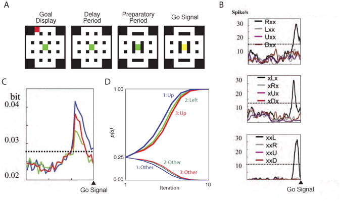
A. Example displays from Mushiake et al. (2006, p. 633), showing the sequential presentation of goal and barrier locations. B. Response profiles of three dorsolateral prefrontal neurons studied by Mushiake et al. (2006, p. 635). The arrowhead on the x-axis indicates the onset of the visual signal cuing the animal to begin navigating the maze. The top panel shows a neuron selective for rightward movement on the first step; the middle panel a neuron selective for leftward movement on the second step; and the lower panel a neuron selective for leftward movement on the third step. C: Data from Mushiake et al., (2006) showing simultaneous emergence, over a population of prefrontal neurons, of information concerning first (blue), second (green) and third (red) actions during planning. D. Results of Simulation 3.3. Numbers indicate the relevant action variable (as though moving from left to right in the architecture shown in Figure 2D). ‘Other’ indicates actions down, right and left on step one and three, and actions up, down and right on step two. Note that Mushiake et al. (2006) also presented data relating to plan execution, which are omitted here.
In order to simulate these results, we implemented a three-stage model. Considering that the action units in our neural network model convey the probability p(a|s), and thus carry the same information as the A variables in our graphical model, for convenience we performed this simulation using the graphical model implementation. The state space included the set of occupiable positions in the maze, with available actions including movement in the four cardinal directions. The transition function dictated that movement into a barrier yielded no change in position, and reward was associated with the single goal location (p(r̂)= 0.7; elsewhere 0.05).
The central result of the simulation is shown in Figure 11D. This shows the evolution of the action posteriors for the first, second and third steps in the plan, as they converge to the correct plan up→left→up. Of course, our model includes conjunctive representations of action and ordinal position, and thus matches this aspect of the empirical data by design. What the figure shows, additionally, is that the decision processes at the three steps follow highly overlapping time-courses, very much in line with the parallel activation observed in the Mushiake et al. (2006) study.
It is revealing to compare these results with those from Simulations 2.1 and 2.2 (see Figures 6E and 6F). The present simulation shows that within our model as in Mushiake's (2006) study, planning at successive steps can be highly parallel in time. Figure 6, in contrast, shows cases where planning is more asynchronous. In Figure 6F, the decision at the first step of a two-step plan emerges first. In Figure 6E the order is reversed, with the decision at the second step evolving faster. As this contrast indicates, although our model can be fit to the findings from Mushiake et al. (2006), the model more generally predicts that the relative timing of decision making across stages of a multi-step plan will vary systematically with the specific set of outcome contingencies involved in the decision task.
3.4 Evidence integration in simple incentive choice
Earlier we compared our graphical model account with evidence integration models of perceptual decision making. We are now in a position to consider this parallel from a neuroscientific point of view. A range of studies have mapped the elements of the evidence-integration framework onto specific neural regions, in the context of specific perceptual tasks. The most extensive research has focused on the dot motion paradigm reviewed earlier and diagrammed in Figure 4. Here, neurophysiological research has focused on localizing two critical functions. The first is the ‘integrator’ itself, the area or areas in which information about visual motion accumulates over time, leading neural activity to approach or retreat from decision thresholds. Activity fitting with this description has been identified in lateral intraparietal area (LIP) as illustrated in Figure 12A, based on work by Gold and Shadlen (2007).
The second focus of neuroscientific work has been to identify the source of input to the integrator, that is, the source of the evidence feeding into the evidence-integration mechanism. Not surprisingly, in the dots task this has been tracked to cortical area MT, which has long been known to encode information concerning visual motion (see Gold & Shadlen, 2001). Unlike neurons in LIP, MT neurons show relatively stable tonic activity during viewing of dot-motion stimuli, consistent with the idea that they are coding for instantaneous information in the display, rather than integrating this information over time (see Figure 12A, inset).
Earlier, we highlighted the fact that the policy variable in our model behaves like an integrator. In this regard, our theory draws a direct analogy between the role of LIP in perceptual decision tasks and the role of DLPFC in goal-directed decision making. The analogy is reinforced in Figure 12B, which shows the activity in the units coding for policy marginals in our neural network model (red in Figure 8), over a set of two-alternative decision problems varying in incentive disparity (see Appendix B for simulation methods).
If the role of DLPFC is analogous to that of LIP in perceptual decision making, then what area is analogous to MT? That is, what area provides the ‘evidence’ that is integrated over time within DLPFC? In formal terms, we earlier identified this evidence with the likelihood p(r̂|π,s). In the setting of simple binary choice, where there is a one-to-one correspondence between actions and outcomes, note that this value is exactly equal to p(r̂|s′). As a consequence, in simple choice, the ‘evidence’ entering into the integration process corresponds to the activation of the units labeled R̂→S′ in our neural network model (purple in Figure 8). In Simulation 3.1, we compared the function of this set of units with that of neurons representing state-value in OFC. The analogue to MT, according to our model, is therefore OFC. The analogy is elaborated in Figure 12B (inset), which shows activity in state-value units for the same choice problems used to generate the policy time-courses above. Like MT, these units show stable tonic activity indicating the ‘strength of evidence’ for one choice over the other.
Predictions
In these simulations, we have focused on cases where signals within the neural network have readily identifiable correlates in the current neuroscientific literature. Other aspects of the neural network model lead to further testable predictions. For example, the units labeled S′→ R̂ and shown in green in Figure 8 represent the probabilities of outcome states.12 The model predicts that such representations should be identifiable within the brain, and (less obviously) that sequence planning should activate neural representations of sequences of future states, with order-specific coding as has been demonstrated for actions (see Simulation 3.3). Some neuroscientific evidence consistent with prospective state coding was discussed earlier. With regard to representation of multiple future states during planning, suggestive evidence is provided by Saito and colleagues (2005), who showed that neurons in prefrontal cortex encode both immediate and final goal locations in parallel during planning in a maze navigation task. Having noted this, it should be acknowledged that other studies have uncovered representations of state that fit less tidily into the present account. Johnson and Redish (2007) observed hippocampal activation apparently coding for projected future positions during path planning. However, in contrast to the activation reported by Saito et al. (2005), these activations were activated serially in time rather than concurrently. In other recent work, Stalnaker and colleagues (2010) reported neurons in dorsal striatum coding for action-outcome conjunctions. Such representations do not figure in our neural network model, and therefore present a challenge to be examined in future work.13
A further prediction stems from the fact that our model posits separate representations of expected reward for each stage in a multi-stage plan. Given the parallels we have drawn to OFC and amygdala, this predicts that similar, step-specific reward representations should be identifiable in one or both of these regions during the planning of sequential actions. To our knowledge, neural activity in these regions has not been studied in the setting of sequence planning (though see Simon & Daw, 2011).
Finally, Simulation 3.2 leads to specific predictions concerning neural action-value representations. In previous work, such representations have generally been assumed to support model-free or habitual action selection (see, e.g., Samejima, et al., 2005). Our model shows how action-value representations might arise during goal-directed decision making. Furthermore, our model suggests a close link between action-value and state-value representations, with the latter providing part of the basis for computing the former during the course of single decision-making episodes (for related proposals, see Hasselmo, 2005). This leads to the novel prediction that disruptions of neural state-value representations, for example in the OFC, should disrupt action-value coding, for example in parietal cortex or striatum.
General Discussion
In the present paper, we have advanced an account of goal-directed decision making. With a nod to David Marr, we have specified the theory at computational, algorithmic and implementational levels. At the computational level, the proposal aligns with contemporary theories in vision, motor control and other domains, which center on inverse inference within a generative model. In the present work, the generative model in question captures the way in which policies, actions, and states work together to generate rewards, and model inversion reveals the policy that best explains the occurrence of reward. The procedures involved in carrying out this inversion link the present account with current theories of perceptual decision making, which center on iterative evidence integration. Like such theories, the present one can be translated into neural terms, providing an account of how populations of neurons spanning relevant brain areas may work together to yield goal-directed decisions. Across the algorithmic and implementational levels, the theory we have presented accounts for a range of behavioral and neurophysiological observations, and gives rise to testable predictions. In this final section, we pan back to consider the relationship between the ideas we have presented and previous work, and enumerate some areas for further development.
Related work in machine learning and theoretical neuroscience
As intimated earlier, although the notion of reward-based decision making as inference has been little explored in psychology or neuroscience, versions of the idea have been in play for several decades within decision theory and machine learning. Initial proposals for how to solve decision problems through probabilistic inference in graphical models, including the idea of encoding reward as the posterior probability of a random utility variable, were put forth by Cooper (1988). Related ideas were presented by Shachter and Peot (1992), including the use of nodes that integrate information from multiple utility nodes. More recently, Attias (2003) and Verma and Rao (2006b) have used graphical models to solve shortest-path problems, leveraging probabilistic representations of rewards, although not in a way that guarantees convergence to reward-maximizing plans. More closely related to the present research is work by Toussaint and Storkey (2006) employing the expectation-maximization algorithm, a technique with interesting but insufficiently explored relations to evidence-integration procedures (see also Dayan & Hinton, 1997; Furmston & Barber, 2009; Hoffman, et al., 2009).
Although close in spirit, our framework does not fully parallel any of this previous work. Perhaps the most important difference is at the level of the research objective: The aim of the present work has been to maximize not computational power but rather explanatory power, by engaging wherever possible with established principles and findings in psychology and neuroscience. Our efforts to relate the present theory to accounts of perceptual decision making and to available functional-neuroanatomic and neurophysiologic data are emblematic of this objective.
Within neuroscience, one recent line of work that has explored reward-based decision making from an inference-centered point of view is by Friston and Daunizeau (2009). This work adopts the generative perspective, proposing that the brain is shaped through learning to minimize its own ‘surprise’ by maximizing the accuracy of its predictions about external inputs. Action selection is then modeled by introducing the additional assumption that the brain is configured to predict the perceptual feedback that would be produced by adaptive actions. The objective of minimizing surprise is then met by selecting actions that assure the predicted inputs. Beyond its shared focus on inference within a generative model, this approach is somewhat different from the one we have taken. In the theory of Friston and colleagues, the role of the central generative model is to predict observations (perceptual inputs), and the role of action is to realize those observations. The generative model at the center of our work is itself the substrate for action selection, accomplished through inverse inference from the fixed initial ‘observation’ of reward. Interestingly, the model of Friston and colleagues (2009) deliberately eschews any explicit representation of reward; reward is encoded implicitly through the distributions that express the agent's predictions. While such an implicit encoding may be computationally feasible (see Furmston & Barber, 2009), it does not square well with the neurophysiological data reviewed earlier (e.g., Padoa-Schioppa & Assad, 2006), which provide strong evidence for explicit neural representations of reward.
Spreading Activation Models of Spatial Navigation
One other area in which some work has been done on the neuro-computational basis of goal-directed decision making is spatial navigation. The predominant approach in such work is represented in studies by Schmajuk and colleagues (Schmajuk & Thieme, 1992; Voicu & Schmajuk, 2002), and subsequent simulations by Hasselmo and colleagues (Hasselmo, 2005; Koene & Hasselmo, 2005). Both sets of models assume a network of simple neuron-like processing elements representing environmental states or locations, which plays the role of the cognitive map. In Schmajuk's models inputs representing incentive value activate rewarded locations, and activation spreads from these locations to adjacent ones until the frontier of activation reaches the agent's current location. This results in an activation map, from which actions can be selected through a hill-climbing procedure (for related work see Bugmann, Taylor, & Denham, 1995; Gaussier, Revel, Banquet, & Babeau, 2002; Girard, Filliat, Meyer, Berthoz, & Guillot, 2005; Martinet, Passot, Fouque, Meyer, & Arleo, 2008; Muller, Stead, & Pach, 1996; Reid & Staddon, 1998). Hasselmo's models (Hasselmo, 2005; Koene & Hasselmo, 2005) follow this same general approach, but allow activation also to spread ‘forward’ from the agent's initial state (see also Smith, et al., 2004). These models also explicitly represent actions and action-outcome relationships, permitting the models, at least in principle, to be applied beyond the domain of spatial navigation.
The framework we have put forth shares a definite family resemblance with such spreading-activation models. In particular, one can relate the propagation of activation within these networks to the message-passing operations within our neural network implementation. A relative strength of our model, once again, is that it offers an explicit formal characterization of the computations involved,14 establishing a link between these computations and inference-based operations in other information-processing domains, as well as to normative and empirical accounts of perceptual decision making. Furthermore, by implementing goal-directed decision making in probabilistic terms, our models also naturally extend to settings involving uncertain outcomes and multiple sources of reward or cost, settings not generally addressed by spreading activation models.
Evidence-integration models of decision making
A key feature of our account is its incorporation of an iterative procedure transparently related to the sequential probability ratio test, an optimal procedure for sequential hypothesis testing. As we have emphasized, this aspect of our model links it closely with current theories of perceptual decision making, in particular those leveraging the drift-diffusion formalism. Our neural-network implementation reinforces this connection, based as it is on a recent effort to translate such decision-making theories into neural terms.
The success of drift-diffusion models in perceptual decision making and other domains has inspired several researchers to apply the same framework to reward-based decisions. In several cases, the proposal has been to import the drift-diffusion model en bloc, simply relabeling the inputs to the process as the utilities of choice objects (Krajbich, Armel, & Rangel, 2010; Rangel, 2008; Rustichini, 2008; Shadlen, 2008). The present work complements and extends such efforts in two ways. First, it furnishes an explicit statistical interpretation for evidence integration in the context of reward-based decision making. In the case of perceptual decision making, such an interpretation is ready to hand: The evidence-integration process is understood as an implementation of the sequential probability ratio test, with perceptual inputs playing the role of the data, representations of stimulus identity playing the role of hypotheses, and a well-characterized likelihood function p(data | hypothesis) linking the two (see Figure 4). In contrast, prior applications of the evidence-integration framework to reward-based decision making have not, to our knowledge, been associated with a corresponding statistical interpretation. The present work bridges this gap. In our framework, the fictive observation r̂ = 1 plays the role of the data; each hypothesis corresponds to the belief that the observation r̂ = 1 is explained by a particular policy; and the likelihood function is p(r̂|π,s).
In addition to providing this formal interpretation for evidence-integration models of reward-based decision, the present work also generalizes the approach. Indeed, the standard drift-diffusion model can be seen as a limiting case of the present framework, which obtains in the setting of two-alternative forced choice with one-to-one, deterministic action-outcome contingencies (see Appendix A). The present account widens the scope of the evidence-integration paradigm to accommodate stochastic action-outcome contingencies and multi-step planning.15
Alongside direct applications of the drift-diffusion model, several models have adapted the evidence-integration framework to reward-based decision in more elaborate and specialized ways. Such work includes the leaky competitive accumulator (LCA) model of Usher and colleagues (Bogacz, Usher, Zhang, & McClelland, 2007; Konstantinos, Usher, & Chater, 2010; Usher, et al., 2008), the decision-by-sampling (DBS) framework of Stewart and colleagues (Stewart, 2009; Stewart, et al., 2006) and decision field theory (DFT), as proposed by Busemeyer and colleagues (Busemeyer & Diederich, 2002; Busemeyer & Townsend, 1993). Our model has features in common with all three of these, given their shared use of sequential sampling, along with integrator-like mechanisms. One important difference is that the LCA, DBS and DFT models all focus heavily on multi-attribute decision making, where choice options are characterized along multiple feature dimensions. Extending the present framework to engage the multi-attribute case is an important area for future development. Elaborating the computational architecture to accommodate multiple feature dimensions is, in itself, quite straightforward, as demonstrated by related work in machine learning using factored state representations (see, e.g., Toussaint & Storkey, 2006). The key question for future work is whether introducing factored representations into the present framework gives rise to patterns seen in human multi-attribute choice (see Busemeyer & Diederich, 2002; Konstantinos, et al., 2010).
Departures from rationality
A central preoccupation in work with the LCA, DBS, DFT and related models has been with putative departures from rationality, as defined by classical expected-value theory. The ability of such models to account for biases and heuristic use in decision making may at first appear to reflect a fundamental difference in approach from the one we have pursued. It is, after all, true that our framing of the goal-directed decision making problem is normative in form, taking the maximization of expected reward (or subjective utility) as its objective. In this respect, the present framework aligns with a wide range of other work that adopts a normative approach to decision making (e.g., Anderson, 1990; Bogacz, et al., 2006; Geisler, 2003; Niv, et al., 2006). A particularly strong resonance is with work taking a normative perspective on action understanding (Bekkering, et al., 2000; Csibra & Gyorgy, 2007; Gergely & Csibra, 2003), some of which has also adopted an explicitly probabilistic approach (Baker, Saxe, & Tenenbaum, 2009; Rao, et al., 2007; Verma & Rao, 2006a).
Having said this, it is also important to note that our account presumes that decision-making is rational only relative to the decision-maker's internal model of the problem (see Simon, 1987). Throughout the present work we have assumed, for simplicity, that this model accurately captures the objective probabilities associated with action-outcome contingencies, and represents reward values in a simple linear fashion (see Equation 8). However, the framework naturally accommodates representations of contingency and reward that depart from this default case. In particular, the distribution p(r̂|s′) could be assumed to have the asymmetric sigmoid form of the utility function posited by prospect theory (Kahneman & Tversky, 1979), and the distribution p(s′|s, a) could be assumed to distort objective outcome probabilities as occurs in prospect theory's weighting function. Under these assumptions, the present model would inherit the ability of prospect theory to account for such phenomena as loss aversion and interactions between outcome probability and valence in determining risk attitude.
This approach of simply ‘plugging in’ functions from prospect theory has precedents in the decision modeling literature (see e.g., Konstantinos, et al., 2010; Usher, et al., 2008), and could arguably be justified in our model — independently of the behavioral phenomena to be explained — based on neurophysiological data identifying neural response profiles resembling those functions (Fox & Poldrack, 2008; Hsu, Krajbich, Zhao, & Camerer, 2009). However, rather than simply stipulating the relevant functional forms, it would perhaps be more satisfying if they could be understood as emerging naturally through learning. The psychology, neuroscience and economics literatures suggest some interesting possibilities in this regard, which may have further relevance to departures from strict rationality, as we discuss next.
Learning
The work we have presented, like most work on goal-directed decision making, has focused on the question of how decisions are made in the presence of an established internal model of the task domain. A truly comprehensive theory would need to include an account of how that internal model arises (see Glascher, et al., 2010; Green, et al., 2010). The theory we have presented is, we believe, quite amenable to such an extension. Indeed, formal methods for learning in graphical models are well-developed (Jordan, 1998), and analogies have already been made between the relevant algorithms and learning processes in humans (Chater, Tenenbaum, & Yuille, 2006; Gopnik & Schulz, 2007).
From a purely formal perspective, the most obvious approach to learning in our graphical model would be to base the CPD at each node on event counts, since these provide maximum-likelihood estimates of the true distributions (see Koller & Friedman, 2009). Thus, for example, if an action a in situation s can lead to two outcomes s′1 and s′2, the transition probabilities could be estimated as the count ratios and . Attias (2003) has demonstrated the feasibility of combining this form of learning with concurrent inference-based decision making.16
However, an appealing alternative approach to learning is suggested by recent work in psychology and economics. As briefly mentioned earlier, in the DBS model of Stewart and colleagues (2009; 2006), continuous quantities such as utilities and outcome probabilities arise out of a tournament-like process. To compute the utility of a particular item, for example, that item is compared against a series of reference items, sampled from memory based on their frequency of occurrence in past experience. The proportion of comparisons in which the index item is judged preferable to the reference item becomes the scalar representation of the index item's utility (for a related proposal in economics, see Kornienko, 2010; Van Praag, 1968).
It seems inviting to consider how this tournament-based approach could be integrated into our framework, for several reasons. First, the approach provides a natural interpretation for our binary representation of reward: p(r̂|s′)could be interpreted as the proportion of ‘victories’ enjoyed by s′ in the relevant tournament. Note that here, because p(r̂|s′) depends on the set of states against which s′ is compared, the value p(r̂|s′) acquires the property of range adaptation (see Kornienko, 2010; Stewart, et al., 2006). This is appealing from a neuroscientific perspective, since recent studies have demonstrated range adaptation in neural representations of reward (Kobayashi & Carvalho, 2010; Padoa-Schioppa, 2009). Range adaptation is also appealing from the point of view of behavioral economics; as Stewart and colleagues (2009; 2006) have detailed, adaptive coding provides an explanation for the emergence of both the utility and weighting functions from prospect theory. Furthermore, because adaptive coding makes the representation of utility (and other quantities) context-dependent, it gives rise to a number of phenomena that present a challenge for standard expected utility (e.g., similarity, compromise and attraction effects; see Busemeyer & Diederich, 2002; Konstantinos, et al., 2010; Kornienko, 2010; Stewart, 2009). Evaluating the potential role for these considerations within the present theory is an important target for future research.
One further germane aspect of learning arises from cognitive research on planning and problem solving. Such work highlights the importance not only of learning about state transitions, but also learning to represent states themselves (Chase & Simon, 1973). The principles underlying such representational or state-space learning (see Gershman & Niv, 2010) are still poorly understood, and incorporating this aspect of learning into models of goal-directed behavior stands as an important long-range challenge.
Capacity limitations, heuristics and problem representation
Cognitive research on planning also highlights another characteristic of human goal-directed decision making that we have not considered thus far: its rather strict capacity limitations. A central take-home message from prior research is that human planners are incapable of reasoning precisely about complex problems, due largely to limitations on working memory capacity, and thus resort to a number of simpler problem-solving heuristics (Newell & Simon, 1972; Novick & Bassok, 2005; Unterrainer & Owen, 2006). One way of understanding such capacity limitations within the present framework would be in terms of a limit on the number of future steps of action that can be concurrently represented. This limit could be a property of the underlying processing architecture, i.e., an inherent limit on the number of segments within the structure posited in Figure 2 (bottom). A structural limit of this flavor has been independently proposed in work on multi-tasking (Koechlin & Hyafil, 2007), and inherent limits on depth of search have also been heavily discussed in work on decision making in economic games (see Camerer, 2003). One reason such a depth limit might make functional sense in the problem settings we have considered relates to the impact of noise. In any model of planning where random variability plays a role, adding a stage to the planning depth will inject more noise into the planning process. Recalling that decision making at each stage of a sequential plan is dependent on other stages, it seems likely that the impact of noise will grow in a non-linear fashion as planning depth increases, making deep search intractable (see Daw, et al., 2005).
Another perspective on capacity limitations that may have relevance within the present account comes from work suggesting that human cognition does not leverage probability distributions in their entirety, but rather only samples from such distributions. Under this approach, capacity limitations in information processing are understood to arise from limitations on the number of samples that can be made during a single decision-making event. This general idea, which leverages machine learning algorithms for approximate inference, has been applied to magnitude estimation (Vul & Pashler, 2008) and sentence processing (Levy, Reali, & Griffiths, 2009).17 The notion of sampling has already entered into the present work, both in connection with random utility and in our neural network implementation. Evaluating the more general relevance of the sampling hypothesis to goal-directed decision making is an inviting area for further theory development.
As noted earlier, the cognitive planning literature not only documents capacity limitations, but goes on to characterize the strategies used by human planners to mitigate or cope with those limitations (Newell & Simon, 1972). Some of the relevant ideas are readily transposed into the present theory. For example, one method of coping with limited or costly processing capacity is to simplify problem representations. This has been proposed, in particular, to explain intransitivities in multi-attribute choice (Kalenscher, Tobler, Huijbers, Daselaar, & Pennartz, 2010; Shah & Oppenheimer, 2008; Tversky, 1969, 1972). Such a strategy would enter into the present theory at the level of the underlying generative model, since this model is in essence a representation of the decision problem. Strategic selection of this model might thus be considered part of an adaptive procedure for goal-directed decision making. Accounting for this model-specification stage presents an important challenge for development of the present theory, as for any theory of goal-directed decision making or planning.
Another planning strategy that helps in overcoming capacity limitations is referred to as hill climbing. Here, a goal is pursued by selecting actions that reduce the discrepancy between the present state and the goal state (Newell & Simon, 1972). Within the present model, this strategy would correspond to imposing a special or auxiliary reward function, which values states in proportion to their similarity to a goal state. Of course, to make good on this proposal, it would be necessary to supplement the present theory with an account of how reward functions might be strategically chosen. Interestingly, this is an issue that comes up in the field of hierarchical reinforcement learning, a field whose relevance to psychology and neuroscience we have recently considered elsewhere (Botvinick, Niv, & Barto, 2009; Ribas-Fernandes, et al., 2011).
Indeed, one further strategy for mitigating the impact of limited capacity on goal-directed decision making, both in machine learning and in human cognition, is through hierarchical representation. Hierarchical action representations simplify the planning problem, allowing plans to reach deeper into the future through efficient coding of action sub-sequences (see Botvinick, Niv, et al., 2009). As discussed in Simulation 2.3, Ostlund and colleagues (2009) reported devaluation behavior which they interpreted as direct evidence for “chunked” action representations in goal-directed behavior. Although, in our earlier discussion, we suggested the relevant data might be explained without chunking, it seems certain that, in the general case, hierarchical action representations do play a role in goal-directed decision making. In recent work, Toussaint, Charlin and Poupart (2008) have provided an initial demonstration of how hierarchical representation can be integrated with inference-based planning. It would be interesting to consider how the relevant computational issues relate to recent findings suggesting that prefrontal cortex houses a topographically organized hierarchy of action representations (Badre, 2008).
Human capacity limitations in planning, as well as the strategies and heuristics used to cope with them, have of course been a central concern in production-system models including ACT-R and SOAR (Anderson, et al., 2004; Laird, Newell, & Rosenbloom, 1987). Such models stand in a complex relationship to models that approach goal-directed decision making from a reinforcement learning perspective, as recently discussed by Dayan (2009). One difference is in the way the underlying problem is typically framed. Production system models, following the tradition in problem-solving research, have tended to focus on tasks defined by an explicit a priori goal. In work inspired by reinforcement learning, including the work we have presented here, specific goal states do not figure at all in the formulation of the computational problem, which focuses instead on the generic goal of reward maximization. Recent versions of SOAR and ACT-R have begun to incorporate representations of reward into their accounts of action selection (see Anderson, et al., 2004; Nason & Laird, 2005). However, in both cases the role of such representations appears to align more with the action values found in model-free reinforcement learning than with the free-standing reward function that is central to model-based or goal-directed action. Of course, this is not to say that production system models could not implement goal-directed choice procedures. Indeed, many ACT-R models contain action-outcome information in declarative memory, and recent work has also used declarative memory for rewards to guide action selection (see Stewart, West, & Lebiere, 2009). The challenge for production system models lies not in any restriction on their representational capacities, but instead in their very flexibility. Such models could, in principle, implement any of a range of procedures for goal-directed decision making; the architectures, in and of themselves, do not furnish a specific theory. Nonetheless, because production system models, and in particular ACT-R, take detailed account of basic cognitive faculties (perhaps most importantly the dynamics of memory), we believe they may offer a useful context in which to compare theories of goal-directed decision making, including the one we have advanced here.
Relations with habitual action selection
In the present work, we have modeled goal-directed decision making in isolation, but as recent work has emphasized, human and animal behavior also rests upon habitual action selection, supported by different computational and neural mechanisms. A final important area for further development of the current account involves the question of how goal-directed decision making mechanisms interface with the habit system (Botvinick & Plaut, 2006; Cooper & Shallice, 2006; Coutureau & Killcross, 2003; Daw, et al., 2005; Killcross & Coutureau, 2003). One way to model the role of habits in the present framework might be as additional inputs to policy variables, biasing policy selection toward habitual configurations. Another potential point of contact between goal-directed and habit mechanisms might also be at the planning horizon: Rather than encoding immediate reward at the final step of a multi-step plan, it might make more sense to represent a cached ‘reward-to-go’ value, a central element in model-free temporal-difference learning algorithms (see Sutton & Barto, 1998). Capping off explicit prospective ‘roll-outs’ with value representations of this kind has become standard in recent machine learning models of forward planning in partially observable domains (see Ross & Pineau, 2008). Whether an application of these ideas within the present framework would align with available behavioral and neural evidence concerning the goal/habit interface will be an interesting question to pursue.
Conclusion
Despite a veritable explosion in computational work addressing habitual action selection, inspired largely by theories linking dopamine with temporal-difference learning, relatively little work has been done to specify the computational principles involved in goal-directed decision making. The present work contributes toward rectifying this imbalance. In addition to adopting the view that goal-directed decision making can be viewed in the terms provided by model-based reinforcement learning, our proposal seeks to account for such decision making in terms that figure equally in other domains of neural information processing, including other types of decision making, motor control, perception, and beyond. By portraying goal-directed decision making as probabilistic inference, the work we have presented fits into to a broad movement within both psychology and neuroscience, which sees inference as providing a lingua franca, applicable across content domains as well as across computational, algorithmic and implementational levels of description (Chater & Oaksford, 2008; Doya, Ishii, Pouget, & Rao, 2006; Jones & Love, 2011).
Given the early stage of computational research on goal-directed decision making, the most important contribution of the present work is simply to chart out one sector in the space of possible computational approaches. By performing this role, we hope the work will, at the very least, provide a useful stepping stone toward further computational and empirical research in this important domain.
Supplementary Material
Acknowledgments
Thanks to James An for contributions to the simulation work, and to David Blei, Peter Dayan, Nathaniel Daw, Andrew Ledvina, Yael Niv, Francisco Pereira, Mike Todd, and participants in the Neural Basis of Goal Directed Behavior seminar at Princeton for useful discussion. The present research was supported by a grant from the McDonnell Foundation to M.B.
Appendix A.
Formal Analysis
The main text introduced an iterative procedure for solving finite horizon Markov decision problems within graphical models of the kind displayed in Figure 2. Here we provide formal proofs of monotonicity and convergence (based on Botvinick & An, 2009), which guarantee that the algorithm will converge to an optimal policy. To recap, the procedure is as follows: (1) Initialize the policy nodes with any set of non-deterministic priors. (2) Treating the initial state and R̂c as observed variables, with r̂c=1, use standard belief propagation or a comparable algorithm to infer the posterior distributions over all policy nodes. (3) Set the prior distributions over the policy nodes to the values (posteriors) obtained in step 2. (4) Go to step 2. The proofs follow:
Monotonicity
We show first that, at each policy node, the probability associated with the optimal policy will rise on every iteration. Define π* as follows:
| (A1) |
where π+ is the current set of probability distributions at all policy nodes at all subsequent steps within the plan (i.e., to the right within the model architecture. Note that we assume here, for simplicity, that there is a unique optimal policy at each step.) The objective is to establish that:
| (A2) |
where n indexes processing iterations. The evidence integration procedure stipulates that
| (A3) |
where π represents any value (i.e., policy) of the decision node being considered. Substituting this into A2 gives
| (A4) |
From this point on the focus is on a single iteration, which permits us to omit the relevant subscripts. Applying Bayes' law to A4 yields
| (A5) |
Canceling, and bringing the denominator up, this becomes
| (A6) |
Rewriting the left hand side, we obtain
| (A7) |
Subtracting and further rearranging:
| (A8) |
| (A9) |
| (A10) |
Note that this last inequality (A10) follows from the definition of π*.
Remark: Of course, the identity of π* depends on π+. In particular, the policy π* will only be part of a globally optimal plan if the set of choices π+ is optimal. Fortunately, this requirement is guaranteed to be satisfied, as long as no upper bound is placed on the number of processing cycles. Recalling that we are considering only finite-horizon problems, note that for policies leading to states with no successors, π+ is empty. Thus π* at the relevant policy nodes is fixed, and is guaranteed to be part of the optimal policy. The proof above shows that π* will continuously rise. Once it reaches a maximum, π* at immediately preceding decisions will perforce fit with the globally optimal policy. The process works backward, in the fashion of backward induction.
Convergence
Continuing with the same notation, we show now that
| (A11) |
Note that, if we apply Bayes' law recursively,
| (A12) |
Thus,
| (A13) |
Therefore, what we wish to prove is
| (A14) |
or, rearranging,
| (A15) |
Note that, given the stipulated relationship between p(π) on each processing iteration and p(π|r̂c) on the previous iteration,
| (A16) |
With this in mind, we can rewrite the left hand side product in A15 as follows:
| (A17) |
Note that, given A16, the numerator in each factor of A17 cancels with the denominator in the subsequent factor, leaving only p(r̂c|π*) in that denominator. The expression can thus be rewritten as
| (A18) |
The objective is then to show that the above equals p1(π*). It proceeds directly from the definition of π* that, for all π other than π*,
| (A19) |
Thus, all but one of the terms in the sum above approach zero, and the remaining term equals p1(π*). Thus,
| (A20) |
Convergence Under Random Utility
We show here that the algorithm will also converge to the optimal policy under random utility. We focus on the single-step model, but the proof can be extended to the multi-step case. As in the main text, we assume that the distribution of the variable R depends jointly on S′ and on a vector-valued random variable Z, whose elements are independent and identically distributed. Z is assumed to be sampled upon each iteration of the evidence-integration procedure described above and in the main text. Define
| (A21) |
where E indicates expectation, and conditioning on the initial state s is implicit. Adopting this definition, the last expression in A18 becomes (replacing r̂c with r̂):
| (A22) |
Given the present definition of π*, to A19 translates to:
| (A23) |
The expected value for the product in A22 is equal to the product of the expected values for the individual factors (iterations) indexed by m. Given A23, the latter product goes to zero as m goes to infinity for every π≠ π*. Thus, the expected value of the left-hand side in A22 must converge to p1(π*). It can be easily shown that the variance of that same expression goes to zero as m goes to infinity, guaranteeing that p(π*) will converge to one.
Relation to Sequential-Sampling Models
The main text asserted a link between the present model and evidence-integration or sequential-sampling models of perceptual decision making, including random walk and drift-diffusion models, which in the case of binary choice are known to implement the sequential probability ratio test (for reviews, see Bogacz, et al., 2006; Gold & Shadlen, 2007). We show here that in the same setting of simple binary choice, the model we have proposed displays precisely the same dynamics. The analog to the decision variable in standard random walk model is the log policy posterior ratio
| (21) |
where πA and πB are the two response options (policy values), and as before n is the iteration, and u is shorthand for u = 1. It is easily shown that in the absence of noise, this value grows linearly with a step size equal to the log likelihood ratio given the evidence r̂=1. The increment in the decision variable on each time step is
| (A22) |
Absorbing the second term into the first, and applying Bayes' law along with the stipulation that pn(π)= pn-1(π|r̂), this becomes
| (A23) |
which reduces to
| (A24) |
This last expression is a constant, confirming that the decision variable grows linearly with a step size equal to the log likelihood ratio.
In our model, ‘drift rate’ variability derives purely from internal sources of noise. In our algorithmic account, the source of noise is understood as deriving from intrinsic variability in the reward function, modeled using the noise variable Z. If the distribution of Z is chosen as in our simulations (see Simulation Methods below), then drift-rate variability assumes a uniform Gaussian form, as in the drift diffusion model.
Appendix B.
Simulation Procedures
Graphical Model
All simulations were run using the Matlab Bayes Net Toolbox (Murphy, 2001), combined with custom Matlab (Mathworks, Natick, MA) code (portions available for download from princeton.edu/∼matthewb).
Simulations addressing single-step decisions employed the architecture from Figure 2C. Multi-step tasks were modeled using the architecture from Figure 2D, extended to include the minimum number of actions required for the task simulated. States, actions and policies were represented by discrete, multinomial variables. Policies were modeled using a set of nodes connected to each action variable, with each node representing the policy for a single state. Each policy-node value corresponded to a unique, deterministic policy for the relevant state. As described earlier, reward was modeled using a binary variable connected to each state variable as described in the main text.
For each task modeled, a scalar reward value R(s′) was assigned to each state s′. The resulting set of reward values was then scaled to fall between zero and one and used to define the CPD for the reward variable, using the linear transformation specified in Equation 8. For simplicity, temporal discounting was not applied, but the framework could accommodate it through appropriate changes to the reward-variable CPD.
Each simulation involved imposing a set of values on one variable or set of variables and computing the posterior distribution over another variable or variables. In all cases, posterior probabilities were computed using the junction tree algorithm (see Jensen, 2001). Iterative inference was conducted as described in the main text and Appendix A. In all simulations, distributions for all policy variables were initialized as uniform.
As shown in Figure 4 (bottom right), Simulation 1.2 included an additional multivariate normal variable Z, with the same dimensionality as S′, and covariance 0.3I. On each iteration of inference, a value of this variable was sampled and treated as observed. The probability p(r̂|s′,z) was then determined as P(logit(ρ)+z), where P is the standard logistic function, z is the value of the element of Z with the same index as s′, and ρ is a parameter p(r̂|s′,0), denoted p(r̂|s′) in the main text.
Neural Network
In translating our generative model into neural network form, we followed the approach outlined by Rao (2005). As noted in the main text, that work proposes how belief propagation might be implemented in biological neural networks, with message components encoded in the proportional firing rates of individual neurons. Following this idea, our neural network models simply implemented standard belief propagation, with a unit for each message component. For a detailed introduction to the operations underlying belief propagation, see Pearl (1988). In what follows, we provide simulation details that cannot be gleaned from this source or from Rao (2005).
The network depicted in Figure 8 was tailored to the two-alternative forced choice task scenario. The messages transmitted within the model were computed as indicated in Table 1. The message m(П;→A) was initialized as 〈0.5, 0.5〉, and updated as:
Table 1. Specification of belief-propagation messages employed in Simulation 3.
| Message | Specification |
|---|---|
| m(S→A,S′) | p(S)*=〈1,0,0〉 |
| m(П→A) | pn(П)= pn−1(П| r̂,s0) |
| m(R̂→S′) | p(r̂|S′) |
| m(S′→A) | m(S′→A)** |
| m(A→П) | p(A| П,s0)m(S′→A) |
| m(A→S′) | α p(A|s0, П)T m(П→A)*** |
| m(S′→ R̂) | α p(S′|s0, A)Tm(A→S′) |
| m(R̂→ R̂c)**** | α p(R̂| S′)Tm(S′→ R̂) |
Here and in subsequent entries, s0 indicates the observed initial state, and the notation p(X) denotes a probability vector with one component for each discrete value of X.
Here and in subsequent entries, p(Y|X) and p(Y|X,z) indicate a matrix with a row for each value of X and a column for each value of Y.
Here and elsewhere, α denotes a normalization factor.
As discussed in the main text (Simulation 3.1), this message derives from the multi-step model.
| (B1) |
where Θ denotes component-wise multiplication. The messages used in the multi-step model can similarly be derived from the general purpose equations prescribed by belief propagation. See Pearl (1988) for details.
Rao (2005) presented an account of how stochasticity in neural firing might enter into a biological implementation of belief propagation. We took a simpler approach, which gives rise to similar network behavior (as confirmed in head-to-head comparison simulations). In our modified approach, rather than treating the marginal probability (p) carried by each message component as an instantaneous firing rate and transmitting its exact value to downstream units, we drew a sample from Binomial(N, p), normalized its value by N (a free parameter, set to 200 in our simulations except where otherwise noted), and transmitted the result. The resulting quantities can be interpreted in two ways. First, they can be interpreted as the proportion of N time-bins within a fixed interval during which an index neuron fired. Alternatively, they can be interpreted as representing the proportion of N neurons, with identical receptive fields, firing within a fixed time-window.
Further details for several specific simulations follow:
Replication of Simulation 1.2 (Figure 8)
Here, a threshold of 0.75 was used along with a value of 75 for the N parameter, and the data presented represent response proportions from a set of 1000 trials.
Simulation 3.2
The approach taken in this simulation was based closely on the procedure followed in Lau and Glimcher (2008). First, one thousand simulation runs were performed for every pairing 〈p(r̂|outcome action 1), p(r̂|outcome action 2)〉 in which each value fell between 0.5 and 0.6, inclusive, and constituted a multiple of 0.01 (threshold parameter = 0.8, N = 200). From each trial, the action chosen and the activation of one S′→A unit at the time of threshold traversal were recorded. The action for which the S′→A unit coded was treated as the ‘preferred’ action in the remaining analysis steps. Following Lau and Glimcher (2008), a logistic regression was conducted to relate the p(r̂|action 1) and p(r̂|action 2) to choice probability (log p(action 1)/p(action 2)). This yielded a regression coefficient of 0.82, i.e.,
| (B2) |
Based on this result, the scale used to represent action value (AV̄)on the x-axis in Figure 10C-D was
| (B3) |
with the quantity 0.5 intended to represent a reference or status quo reward value. Again following Lau and Glimcher (2008), the values plotted on the y axis in Figure 10 represent the residuals ε from two linear regressions:
| (B4) |
Simulation 3.4
The data presented in Figure 12B are based on 50 simulation trials for each reward-value pairing, using a response threshold of 0.8 and N = 200.
Footnotes
As detailed in the General Discussion, the idea that we will pursue also has precedents in machine learning, although it does not yet figure among the standard approaches to solving sequential decision problems.
Representing state as a multinomial variable is obviously a massive simplification. However, the graphical model formalism can accommodate richer representations of state, including factored or distributed representations and representations involving continuously valued features. The same comment applies to the action representations discussed below.
In the present case, where only a single step of action is planned and the initial state is known, there is in fact no need to distinguish between action and policy variables. However, we include policy variables for two reasons. First, they allow the model to accommodate situations where the initial state is uncertain at the time of planning. This is often the case, for example, in behavioral experiments where a participant must prepare to respond to an impending stimulus, without yet knowing the exact identity of the stimulus. Indeed, this is precisely the scenario involved in most experiments that have demonstrated coding for specific tasks in prefrontal cortex (see Neural Implementation). Second, we include policy variables for parallelism with the multistep case, where they are in fact computationally necessary.
From here forward, to avoid clutter, we suppress the noise variable Z.
In the evidence-integration framework one has a fixed likelihood function and stochastic observations. In the present model, one has instead a fixed observation and a stochastic likelihood function. Mathematically, these two cases are notational variants of one another.
Note that the rat's ‘state’ at S2 and S3 might thus be understood as factoring in an internal representation of past actions. However, as Ostlund and colleagues (2009) note, this is not strictly necessary, since visual, tactile, and proprioceptive information might suffice to discriminate among the relevant situations.
It is worth remarking that the computational account we are offering here for the findings of Ostlund et al. (2009) differs from those authors' own interpretation. Ostlund and colleagues considered the observed pattern of behavior to indicate the involvement of “chunked” representations of action sequences. The present simulation illustrates that chunking is not in fact necessary. Having noted this, however, we hasten to add that chunked or hierarchical representations are nonetheless likely to play a role in goal-directed decision making, a point to which we shall return in the General Discussion.
It should be noted that our model intends ‘state’ to encompass not only ambient environmental circumstances, but also internal state, including the state of working memory (implicating relevant DLPFC and parietal areas), affective state (amygdala, insula and other affect-related structures), and homeostatic conditions (hypothalamus).
Although we have focused on OFC and BLA as substrates for the representation of utility, it should be noted that there is evidence that the costs of effort, as studied in Simulation 2.2, may be represented in different structures, in particular the dorsal anterior cingulate cortex (Botvinick, Huffstetler, & McGuire, 2009; Rudebeck, Walton, Smyth, Bannerman, & Rushworth, 2006).
The scheme from Rao (2005) carries with it two particularly speculative assumptions, which it is important to acknowledge. First, it requires multiplicative interactions between pre-synaptic neurons. Although both modeling and empirical work have begun to shed light on how this might be accomplished (Mel, 1992, 1993; Polsky, Mel, & Schiller, 2004), further work is necessary to elucidate the details of these mechanisms. Second, this approach assumes that dendrites are able to approximate a logarithmic transformation (see Rao, 2005 for discussion).
The minor differences between Figure 8B and 6E arise from the fact that an exact algorithm was used in Simulation 2 (see Appendix B). Belief propagation is, technically speaking, an approximate inference algorithm in graphs that contain loops, and so is not guaranteed to yield marginals precisely equivalent to those arising from exact algorithms (see Koller & Friedman, 2009).
Interestingly, these messages represent the probability of states conditional on the current policy distribution, but not on r̂=1. As a result, the predictions represented here do not show the same ‘optimistic’ bias as the marginal state probabilities discussed under Predictions following Simulations 1-2. Another set of messages, present when the model is expanded to encompass more than one step of action, do show the ‘optimism’ effect. Thus, the framework predicts that it should be possible to find multiple representations of outcome probability, some of which are, and some of which are not, optimistic. Some evidence in favor of this kind of multiple coding is reported by Kool et al. (submitted)
One interesting possibility, which was intimated by the Stalnaker and colleagues (2010), is that these neurons are involved in representing the transition function. This is consistent with the finding, from this same study, that many striatal neurons coded in a tonic fashion for the specific response-outcome associations active during the current block of trials.
Hasselmo (2005) discusses parallels between his model and the policy iteration procedure in reinforcement learning. Interestingly, some underlying links to policy iteration have also been considered in planning-as-inference (see, in particular, Toussaint and Storkey, 2006). Further exploring this underlying formal connection would be of interest.
The statistical interpretation offered above for the one-step scenario transfers to the multi-step case: The likelihood in this instance, at each stage t of the plan is p(πt|r̂c,πτ≠t) The optimality property that obtains in the one-step case does not transfer. To our knowledge, optimal decision-making (in the sense involved in the SPRT) has not been studied in the setting of multi-step planning. This strikes us as a fascinating area for future study, into which the present work may provide a portal.
One interesting issue that arises when learning and action selection are interleaved is that action choices can affect what is learned. The learner can thus engage in ‘active learning,’ in which actions are taken to maximize information gain (Castro, et al., 2008; Kruschke, 2008; Steyvers, Tenenbaum, Wagenmakers, & Blum, 2003). Another setting where action can be motivated by the ‘value of information’ is partial observability, where the state of the environment is not entirely available to immediate perception (Behrens, Woolrich, Walton, & Rushworth, 2007; Howard, 1966). The models we presented assumed full state observability. However, Toussaint (2006) and Furmston and Barber (2009) have described how similar principles can be applied to partially observable problems. Evaluating the fit between the resulting account and human behavior in analogous task contexts presents an interesting challenge.
One interesting aspect of sampling-based techniques for approximate inference in graphical models is that they are inherently serial in operation, in some cases involving ‘particles’ that traverse the graphical structure in a wave-like fashion (see Koller & Friedman, 2009). Exploring the application of such procedures in the present modeling context may thus allow contact with evidence that planning in challenging circumstances can take a serial form, often involving serial subgoaling.
References
- Adams C. Variations in the sensitivity of instrumental responding to reinforcer devaluation. Quarterly Journal of Experimental Psychology. 1982;34B:77–98. [Google Scholar]
- Adams CD, Dickinson A. Instrumental responding following reinforcer devaluation. Quarterly Journal of Experimental Psychology: Comparative and Physiological Psychology. 1981;33:109–121. [Google Scholar]
- Anderson JR. The adaptive character of thought. NJ: Erlbaum; 1990. [Google Scholar]
- Anderson JR, Albert MV, Fincham JM. Tracing problem solving in real time: fMRI analysis of the subject-paced tower of Hanoi. Journal of Cognitive Neuroscience. 2005;17:1261–1274. doi: 10.1162/0898929055002427. [DOI] [PubMed] [Google Scholar]
- Anderson JR, Bothell D, Byrne MD, Scott D, Lebiere C, Qin Y. An integrated theory of mind. Psychological Review. 2004;111:1036–1060. doi: 10.1037/0033-295X.111.4.1036. [DOI] [PubMed] [Google Scholar]
- Arana FS, Parkinson JA, Hinton E, Holland AJ, Owen AM, Roberts AC. Dissociable contributions of the human amygdala and orbitofrontal cortex to incentive motivation and goal selection. Journal of Neuroscience. 2003;23:9632–9638. doi: 10.1523/JNEUROSCI.23-29-09632.2003. [DOI] [PMC free article] [PubMed] [Google Scholar]
- Asaad WF, Rainer G, Miller EK. Task-specific neural activity in the primate prefrontal cortex. Journal of Neurophysiology. 2000;84:451–459. doi: 10.1152/jn.2000.84.1.451. [DOI] [PubMed] [Google Scholar]
- Atance CM, O'Neill DK. Episodic future thinking. Trends in Cognitive Sciences. 2001;5:533–539. doi: 10.1016/s1364-6613(00)01804-0. [DOI] [PubMed] [Google Scholar]
- Attias H. Planning by probabilistic inference. Paper presented at the Proceedings of the 9th Int Workshop on Artificial Intelligence and Statistics 2003 [Google Scholar]
- Badre D. Cognitive control, hierarchy, and the rostro–caudal organization of the frontal lobes. Trends in Cognitive Sciences. 2008;12:193–200. doi: 10.1016/j.tics.2008.02.004. [DOI] [PubMed] [Google Scholar]
- Baker CL, Saxe RR, Tenenbaum JB. Action understanding as inverse planning. Cognition. 2009;113:329–349. doi: 10.1016/j.cognition.2009.07.005. [DOI] [PubMed] [Google Scholar]
- Ballard DH, Hinton GE, Sejnowski TJ. Parallel visual computatation. Nature. 1983;306:21–26. doi: 10.1038/306021a0. [DOI] [PubMed] [Google Scholar]
- Balleine BW. Instrumental performance following a shift in primary motivation depends on incentive training. Journal of Experimental Psychology: Animal Behavior Processes. 1992;18:236–250. [PubMed] [Google Scholar]
- Balleine BW. Neural bases of food-seeking: affect, arousal and reward in corticostriatolimbic circuits. Physiology and Behavior. 2005;86:717–730. doi: 10.1016/j.physbeh.2005.08.061. [DOI] [PubMed] [Google Scholar]
- Balleine BW, Dickinson A. The role of cholecystokinin in the motivational control of instrumental action. Behavioral Neuroscience. 1994;108:590–605. doi: 10.1037//0735-7044.108.3.590. [DOI] [PubMed] [Google Scholar]
- Balleine BW, Dickinson A. Goal-directed instrumental action: contingency and incentive learning and their cortical substrates. Neuropharmacology. 1998a;37:407–419. doi: 10.1016/s0028-3908(98)00033-1. [DOI] [PubMed] [Google Scholar]
- Balleine BW, Dickinson A. The interface between affect and cognition Consciousness and Human Identity. Oxford, UK: Oxford University Press; 1998b. pp. 57–85. [Google Scholar]
- Balleine BW, Dickinson A. The role of incentive learning in instrumental outcome revaluation by sensory-specific satiety. Animal Learning and Behavior. 1998c;26:46–59. [Google Scholar]
- Balleine BW, Dickinson A. The role of incentive learning in instrumental outcome revaluation by specific satiety. Animal Learning and Behavior. 1998d;26:46–59. [Google Scholar]
- Balleine BW, Killcross AS, Dickinson A. The effect of lesions of the basolateral amygdala on instrumental conditioning. Journal of Neuroscience. 2003;15:666–675. doi: 10.1523/JNEUROSCI.23-02-00666.2003. [DOI] [PMC free article] [PubMed] [Google Scholar]
- Bargh JA, Green M, Fitzsimons G. The selfish goal. Social Cognition. 2008;26:534–554. doi: 10.1521/soco.2008.26.5.534. [DOI] [PMC free article] [PubMed] [Google Scholar]
- Barlow HB. Pattern recognition and the responses of sensory neurons. Annals of the New York Academy of Sciences. 1969;156:872–881. doi: 10.1111/j.1749-6632.1969.tb14019.x. [DOI] [PubMed] [Google Scholar]
- Barone P, Joseph JP. Prefrontal cortex and spatial sequencing in macaque monkey. Experimental Brain Research. 1989;78:447–464. doi: 10.1007/BF00230234. [DOI] [PubMed] [Google Scholar]
- Barto AG. Adaptive critics and the basal ganglia. In: Houk JC, Davis J, Beiser D, editors. Models of Information Processing in the Basal Ganglia. Cambridge, MA: MIT Press; 1995. pp. 215–232. [Google Scholar]
- Barto AG, Sutton RS. Toward a modern theory of adaptive networks: Expectation and prediction. Psychological Review. 1981;88:135–170. [PubMed] [Google Scholar]
- Baxter MG, Murray AE. The amygdala and reward. Nature Reviews Neuroscience. 2002;3:563–573. doi: 10.1038/nrn875. [DOI] [PubMed] [Google Scholar]
- Baxter MG, Parker A, Lindner CCC, Izquierdo AD, Murray EA. Control of response selection by reinforcer value requires interaction of amygdala and orbital prefrontal cortex. Journal of Neuroscience. 2000;20:4311–4319. doi: 10.1523/JNEUROSCI.20-11-04311.2000. [DOI] [PMC free article] [PubMed] [Google Scholar]
- Beck JM, Pouget A. Exact inferences in a neural implementation of a hidden Markov model. Neural Computation. 2007;19:1344–1361. doi: 10.1162/neco.2007.19.5.1344. [DOI] [PubMed] [Google Scholar]
- Behrens TEJ, Woolrich MW, Walton ME, Rushworth MFS. Learning the value of information in an uncertain world. Nature Neuroscience. 2007;10:1214–1221. doi: 10.1038/nn1954. [DOI] [PubMed] [Google Scholar]
- Bekkering H, Wohlschlager A, Gattis M. Imitation of gestures in children is goal-directed. Quarterly Journal of Experimental Psychology. 2000;53:153–164. doi: 10.1080/713755872. [DOI] [PubMed] [Google Scholar]
- Bertsekas DP, Tsitsiklis JN. Neuro-dynamic programming. Belmont, MA: Athena Scientific; 1996. [Google Scholar]
- Bishop CM. Pattern Recognition and Machine Learning. New York: Springer; 2006. [Google Scholar]
- Blaisdell AP, Sawa K, Leising KJ, Waldmann MR. Causal reasoning in rats. Science. 2006;311:1020–1022. doi: 10.1126/science.1121872. [DOI] [PubMed] [Google Scholar]
- Blodgett HC. The effect of the introduction of reward upon the maze performance of rats. University of California Publications in Psychology. 1929;4:113–134. [Google Scholar]
- Bogacz R, Brown E, Moehlis J, Holmes P, Cohen JD. The physics of optimal decision making: a formal analysis of models of performance in two-alternative forced-choice tasks. Psychological Review. 2006;113:700–765. doi: 10.1037/0033-295X.113.4.700. [DOI] [PubMed] [Google Scholar]
- Bogacz R, Usher M, Zhang J, McClelland JL. Extending a biologically inspired model of choice: Multi-alternatives, nonlinearity and value-based multidimensional choice. Philosophical Transactions of the Royal Society, Series B: Biological Sciences. 2007;362:1655–1670. doi: 10.1098/rstb.2007.2059. [DOI] [PMC free article] [PubMed] [Google Scholar]
- Botvinick M, An J. Goal-directed decision making in prefrontal cortex: A computational framework. Advances in Neural Information Processing Systems. 2009;21 [PMC free article] [PubMed] [Google Scholar]
- Botvinick M, Plaut DC. Such stuff as habits are made on: A reply to Cooper and Shallice (2006) Psychological Review. 2006 under review. [Google Scholar]
- Botvinick MM. Hierarchical models of behavior and prefrontal function. Trends in Cognitive Sciences. 2008;12:201–208. doi: 10.1016/j.tics.2008.02.009. [DOI] [PMC free article] [PubMed] [Google Scholar]
- Botvinick MM, Huffstetler S, McGuire JC. Effort discounting in human nucleus accumbens. Cognitive, Affective and Behavioral Neuroscience. 2009;9:16–27. doi: 10.3758/CABN.9.1.16. [DOI] [PMC free article] [PubMed] [Google Scholar]
- Botvinick MM, Niv Y, Barto AC. Hierarchically organized behavior and its neural foundations: a reinforcement-learning perspective. Cognition. 2009;113:262–280. doi: 10.1016/j.cognition.2008.08.011. [DOI] [PMC free article] [PubMed] [Google Scholar]
- Botvinick MM, Plaut DC. Empirical and computational support for context-dependent representations of serial order. Psychological Review. 2009;116:998–1002. doi: 10.1037/a0017113. [DOI] [PubMed] [Google Scholar]
- Bray S, Shimojo S, O'Doherty JP. Human medial orbitofrontal cortex is recruited during experience of imagined and real rewards. Journal of Neurophysiology. 2010;103:2506–2512. doi: 10.1152/jn.01030.2009. [DOI] [PubMed] [Google Scholar]
- Buckner RL, Carroll DC. Self-projection and the brain. Trends in Cognitive Sciences. 2006;11:49–57. doi: 10.1016/j.tics.2006.11.004. [DOI] [PubMed] [Google Scholar]
- Bugmann G, Taylor JG, Denham MJ. Route finding by neural nets. In: Taylor JG, editor. Neural Networks. Henley-on-Thames: Waller; 1995. pp. 217–230. [Google Scholar]
- Bunge SA. How we use rules to select actions: a review of evidence from cognitive neuroscience. Cognitive, Affective and Behavioral Neuroscience. 2004;4:564–579. doi: 10.3758/cabn.4.4.564. [DOI] [PubMed] [Google Scholar]
- Bunge SA, Wallis JD. The Neuroscience of Rule-Guided Behavior. Oxford, UK: Oxford University Press; 2007. [Google Scholar]
- Bunge SA, Wallis JD, Parker A, Brass M, Crone EA, Hoshi E, et al. Neural circuitry underlying rule use in humans and nonhuman primates. Journal of Neuroscience. 2005;25:10347–10350. doi: 10.1523/JNEUROSCI.2937-05.2005. [DOI] [PMC free article] [PubMed] [Google Scholar]
- Busemeyer J. Decision making under uncertainty: a comparison of simple scalability, fixed-sample and sequential-sampling models. Journal of Experimental Psychology: Learning, Memory and Cognition. 1985;11:538–564. doi: 10.1037//0278-7393.11.3.538. [DOI] [PubMed] [Google Scholar]
- Busemeyer JR, Diederich A. Survey of decision field theory. Mathematical Social Sciences. 2002;43:345–370. [Google Scholar]
- Busemeyer JR, Townsend JT. Decision field theory: a dynamic-cognitive approach to decision making in an uncertain enviroment. Psychological Review. 1993;100:432–459. doi: 10.1037/0033-295x.100.3.432. [DOI] [PubMed] [Google Scholar]
- Camerer C. Behavioral studies of strategic thinking in games. Trends in Cognitive Sciences. 2003;7:225–231. doi: 10.1016/s1364-6613(03)00094-9. [DOI] [PubMed] [Google Scholar]
- Carpenter RHS, Williams MLL. Neural computation of the log likelihood in control of saccadic eye movements. Nature. 1981;377:59–62. doi: 10.1038/377059a0. [DOI] [PubMed] [Google Scholar]
- Castro R, Kalish C, Nowak R, Quian R, Rogers T, Zhu X. Human active learning. Paper presented at the Advances in Neural Information Processing Systems 2008 [Google Scholar]
- Cavada C, Company T, Tejedor J, Cruz-Rizzolo J, Reinoso-Suarez F. The anatomical connections of the macaque monkey orbitofrontal cortex: a review. Cerebral Cortex. 2000;10:220–242. doi: 10.1093/cercor/10.3.220. [DOI] [PubMed] [Google Scholar]
- Chase WG, Simon HA. Perception in chess. Cognitive Psychology. 1973;4:55–81. [Google Scholar]
- Chater N, Manning CD. Probabilistic models of language processing and acquisition. Trends in Cognitive Sciences. 2006;10:335–344. doi: 10.1016/j.tics.2006.05.006. [DOI] [PubMed] [Google Scholar]
- Chater N, Oaksford M. The probabilistic mind: prospects for a Bayesian cognitive science. Oxford: Oxford University Press; 2008. [Google Scholar]
- Chater N, Tenenbaum JB, Yuille A. Probabilistic models of cognition: conceptual foundations. Trends in Cognitive Sciences. 2006;10(7):287–291. doi: 10.1016/j.tics.2006.05.007. [DOI] [PubMed] [Google Scholar]
- Colwill RM, Rescorla RA. Instrumental responding remains sensitive to reinforcer devaluation after extensive training. Journal of Experimental Psychology: Animal Behavior Processes. 1985a;11:520–536. [PubMed] [Google Scholar]
- Colwill RM, Rescorla RA. Postconditioning devaluation of reinforcer affects instrumental responding. Journal of Experimental Psychology: Animal Behavior Processes. 1985b;11:120–132. [PubMed] [Google Scholar]
- Colwill RM, Rescorla RA. Associative structures in instrumental learning. In: Bower GH, editor. The Psychology of Learning and Motivation. Vol. 20. 1986. pp. 55–104. [Google Scholar]
- Colwill RM, Rescorla RA. The role of response-reinforcement associations increases throughout extended instrumental training. Animal Learning and Behavior. 1988;16:105–111. [Google Scholar]
- Cooper GF. A method for using belief networks as influence diagrams; Paper presented at the Fourth Workshop on Uncertainty in Artificial Intelligence, University of Minnesota; Minneapolis. 1988. [Google Scholar]
- Cooper RP, Shallice T. Hierarchical schemas and goals in the control of sequential behavior. Psychological Review. 2006 doi: 10.1037/0033-295X.113.4.887. [DOI] [PubMed] [Google Scholar]
- Corbit LH, Balleine BW. The role of prelimbic cortex in instrumental conditioning. Behavioral Brain Research. 2003;146:145–157. doi: 10.1016/j.bbr.2003.09.023. [DOI] [PubMed] [Google Scholar]
- Corbit LH, Balleine BW. Double dissociation of basolateral and central amygdala lesions on the general and outcome-specific forms of Pavlovian-instrumental transfer. Journal of Neuroscience. 2005;25:962–970. doi: 10.1523/JNEUROSCI.4507-04.2005. [DOI] [PMC free article] [PubMed] [Google Scholar]
- Corbit LH, Ostlund SB, Balleine BW. Sensitivity to instrumental contingency degradation is mediated by the entorhinal cortex and its efferents via the dorsal hippocampus. Journal of Neuroscience. 2002;22:10976–10984. doi: 10.1523/JNEUROSCI.22-24-10976.2002. [DOI] [PMC free article] [PubMed] [Google Scholar]
- Coutureau E, Killcross S. Inactivation of the infralimbic prefrontal cortex reinstates goal-directed responding in overtrained rats. Behavioral Brain Research. 2003;146:167–174. doi: 10.1016/j.bbr.2003.09.025. [DOI] [PubMed] [Google Scholar]
- Csibra G, Gyorgy G. ‘Obsessed with goals’: functions and mechanisms of teleological interpretation of actions in humans. Acta Psychologica. 2007;124:60–78. doi: 10.1016/j.actpsy.2006.09.007. [DOI] [PubMed] [Google Scholar]
- Daw N, Gershman SJ, Seymour B, Dayan P, Dolan RJ. Model-based influences on humans' choices and striatal prediction errors. Neuron. 2011;69:1204–1215. doi: 10.1016/j.neuron.2011.02.027. [DOI] [PMC free article] [PubMed] [Google Scholar]
- Daw ND, Niv Y, Dayan P. Uncertainty-based competition between prefrontal and striatal systems for behavioral control. Nature Neuroscience. 2005;8:1704–1711. doi: 10.1038/nn1560. [DOI] [PubMed] [Google Scholar]
- Dayan P. Goal-directed control and its antipodes. Neural Networks. 2009;22:213–219. doi: 10.1016/j.neunet.2009.03.004. [DOI] [PubMed] [Google Scholar]
- Dayan P, Hinton G, Zemel R. The Helmholtz Machine. Neural Computation. 1995;7:889–904. doi: 10.1162/neco.1995.7.5.889. [DOI] [PubMed] [Google Scholar]
- Dayan P, Hinton GE. Using expectation-maximization for reinforcement learning. Neural Computation. 1997;9:271–278. [Google Scholar]
- Dayan P, Niv Y. Reinforcement learning: the good, the bad and the ugly. Current Opinion in Neurobiology. 2008;18:185–196. doi: 10.1016/j.conb.2008.08.003. [DOI] [PubMed] [Google Scholar]
- De Araujo IET, Kringelbach ML, Rolls ET, McGlone F. Human cortical responses to water in the mouth, and effects of thirst. Journal of Neurophysiology. 2003;90:1965–1876. doi: 10.1152/jn.00297.2003. [DOI] [PubMed] [Google Scholar]
- Deneve S. Bayesian spiking neurons I: Inference. Neural Computation. 2008;20:91–117. doi: 10.1162/neco.2008.20.1.91. [DOI] [PubMed] [Google Scholar]
- Diba K, Buzsaki G. Forward and reverse hippocampal place-cell sequences during ripples. Nature Neuroscience. 2007;10:1241–1242. doi: 10.1038/nn1961. [DOI] [PMC free article] [PubMed] [Google Scholar]
- Dickinson A. Actions and habits: the development of behavioral autonomy. Philosophical Transactions of the Royal Society (London), Series B. 1985;308:67–78. [Google Scholar]
- Dickinson A, Balleine BW. Actions and responses: the dual psychology of behavior. In: Eilan N, McCarthy R, Brewer B, editors. Spatial Representation. Oxford, England: Blackwell; 1993. pp. 276–293. [Google Scholar]
- Dickinson A, Dawson G. Incentive learning and the motivational control of instrumental performance. Quarterly Journal of Experimental Psychology. 1989;41B:99–112. [Google Scholar]
- Dickinson A, Mulatero CW. Reinforcer specificity of the suppression of instrumental performance on a non-contingent schedule. Behavioral Processes. 1989;19:167–180. doi: 10.1016/0376-6357(89)90039-9. [DOI] [PubMed] [Google Scholar]
- Dorris MC, Glimcher PW. Activity in posterior parietal cortex is correlated with the relative subjective desirability of action. Neuron. 2004;44:365–378. doi: 10.1016/j.neuron.2004.09.009. [DOI] [PubMed] [Google Scholar]
- Dosenbach N, Visscher K, Palmer E, Miezin F, Wenger K, Kang H, et al. A Core System for the Implementation of Task Sets. Neuron. 2006;50:799–812. doi: 10.1016/j.neuron.2006.04.031. [DOI] [PMC free article] [PubMed] [Google Scholar]
- Doya K. What are the computations of the cerebellum, the basal ganglia and the cerebral cortex? Neural Networks. 1999;12:961–974. doi: 10.1016/s0893-6080(99)00046-5. [DOI] [PubMed] [Google Scholar]
- Doya K, Ishii S, Pouget A, Rao RPN, editors. The Bayesian Brain: Probabilistic Approaches to Neural Coding. Cambridge, MA: MIT Press; 2006. [Google Scholar]
- Duncan J, Emslie H, Williams P, Johnson R, Freer C. Intelligence and the frontal lobe: the organization of goal directed behavior. Cognitive Psychology. 1996;30:257–303. doi: 10.1006/cogp.1996.0008. [DOI] [PubMed] [Google Scholar]
- Fox CF, Poldrack RA. Prospect theory and the brain. In: Glimcher PW, Fehr E, Poldrack R, editors. Neuroeconomics: Decision Making and the Brain. 145-174. New York: Elsevier; 2008. [Google Scholar]
- Frank MJ, Claus ED. Anatomy of a decision: Striato-orbitofrontal interactions in reinforcement learning, decision making, and reversal. Psychological Review. 2006;113:300–326. doi: 10.1037/0033-295X.113.2.300. [DOI] [PubMed] [Google Scholar]
- Friston KJ. A theory of cortical responses. Philosophical Transactions of the Royal Society of London B Biological Sciences. 2005;350:815–836. doi: 10.1098/rstb.2005.1622. [DOI] [PMC free article] [PubMed] [Google Scholar]
- Friston KJ, Daunizeau J. Reinforcement learning or active inference. PloS One. 2009;4:1–13. doi: 10.1371/journal.pone.0006421. [DOI] [PMC free article] [PubMed] [Google Scholar]
- Furmston T, Barber D. Solving deterministic policy (PO)MDPs using expectation-maximization and antifreeze. Paper presented at the Workshop on Learning and Data Mining for Robotics 2009 [Google Scholar]
- Fuster JM. The prefrontal cortex: Anatomy, physiology, and neuropsychology of the frontal lobe. Philadelphia, PA: Lippincott-Raven; 1997. [Google Scholar]
- Gaussier P, Revel A, Banquet JP, Babeau V. From view cells to place cells to cognitive map learning: processing stages of the hippocampal system. Biological Cybernetics. 2002;86:15–28. doi: 10.1007/s004220100269. [DOI] [PubMed] [Google Scholar]
- Geisler WS. Ideal observer analysis. In: Chalupa LM, editor. The Visual Neurosciences. Cambridge: MIT Press; 2003. pp. 825–838. [Google Scholar]
- Gergely G, Csibra G. Teleological reasoning in infancy: the naive theory of rational action. Trends in Cognitive Sciences. 2003;7:287–292. doi: 10.1016/s1364-6613(03)00128-1. [DOI] [PubMed] [Google Scholar]
- Gershman SJ, Niv Y. Learning latent structure: carving nature at its joints. Current opinion in neurobiology. 2010;20:251–256. doi: 10.1016/j.conb.2010.02.008. [DOI] [PMC free article] [PubMed] [Google Scholar]
- Girard B, Filliat D, Meyer JA, Berthoz A, Guillot A. Integration of navigation and action selection functionalities in a computational model of cortico-basal ganglia-thalamo-cortical loops. Adaptive Behavior. 2005;13:115–130. [Google Scholar]
- Glascher J, Daw N, Dayan P, O'Doherty JP. States versus rewards: Dissociable neural prediction error signals underlying model-based and model-free reinforcement learning. Neuron. 2010;66:585–595. doi: 10.1016/j.neuron.2010.04.016. [DOI] [PMC free article] [PubMed] [Google Scholar]
- Glimcher PW. Choice: Toward a standard back-pocket model. In: Glimcher PW, Camerer CF, Fehr E, Poldrack RA, editors. Neuroeconomics: decision making and the brain. Oxford; Academic Press; 2009. pp. 503–521. [Google Scholar]
- Glymour C. The Mind's Arrows: Bayes Nets and Graphical Causal Models in Psychology. Cambridge: MIT Press; 2001. [Google Scholar]
- Goel V, Grafman J. Are the frontal lobes implicated in “planning” functions? Interpreting data from the Tower of Hanoi. Neuropsychologia. 1995;33:623–642. doi: 10.1016/0028-3932(95)90866-p. [DOI] [PubMed] [Google Scholar]
- Gold JI, Shadlen MN. Neural computations that underlie decisions about sensory stimuli. Trends in Cognitive Sciences. 2001;5:10–16. doi: 10.1016/s1364-6613(00)01567-9. [DOI] [PubMed] [Google Scholar]
- Gold JI, Shadlen MN. The neural basis of decision making. Annual Review of Neuroscience. 2007;30:535–574. doi: 10.1146/annurev.neuro.29.051605.113038. [DOI] [PubMed] [Google Scholar]
- Gopnik A, Glymour C, Sobel D, Schulz T, Kushnir T, Danks D. A theory of causal learning in children: causal maps and Bayes nets. Psychological Review. 2004;111:1–31. doi: 10.1037/0033-295X.111.1.3. [DOI] [PubMed] [Google Scholar]
- Gopnik A, Schulz L, editors. Causal Learning: Psychology, Philosophy, and Computation. Oxford, UK: Oxford University Press; 2007. [Google Scholar]
- Gottfried JA, O'Doherty J, Dolan RJ. Encoding predictive reward value in human amygdala and orbitofrontal cortex. Science. 2003;301:1104–1107. doi: 10.1126/science.1087919. [DOI] [PubMed] [Google Scholar]
- Green CS, Benson C, Kersten D, Schrater P. Alterations in choice behavior by manipulations of a world model. Proceedings of the National Academy of Sciences. 2010;37:16401–16406. doi: 10.1073/pnas.1001709107. [DOI] [PMC free article] [PubMed] [Google Scholar]
- Griffiths TL, Steyvers M, Tenenbaum JB. Topics in semantic representation. Psychological Review. 2007;114:211–244. doi: 10.1037/0033-295X.114.2.211. [DOI] [PubMed] [Google Scholar]
- Gul F, Pesendorfer W. Random expected utility. Econometrica. 2006;74:121–146. [Google Scholar]
- Haber SN, Kim KS, Mailly P, Calzavara R. Reward-related cortical inputs define a large striatal region in primates that interface with associative cortical connections. Journal of Neuroscience. 2006;26:8368–8376. doi: 10.1523/JNEUROSCI.0271-06.2006. [DOI] [PMC free article] [PubMed] [Google Scholar]
- Hamilton AFdC, Grafton ST. Goal representations in human anterior intraparietal sulcus. Journal of Neuroscience. 2006;26:1133–1137. doi: 10.1523/JNEUROSCI.4551-05.2006. [DOI] [PMC free article] [PubMed] [Google Scholar]
- Hamilton AFdC, Grafton ST. Action outcomes are represented in human inferior frontoparietal cortex. Cerebral Cortex. 2008;18:1160–1168. doi: 10.1093/cercor/bhm150. [DOI] [PubMed] [Google Scholar]
- Hassabis D, Kumaran d, Vann SD, Maguire EA. Patients with hippocampal amnesia cannot imagine new experiences. PNAS. 2007;104:1726–1731. doi: 10.1073/pnas.0610561104. [DOI] [PMC free article] [PubMed] [Google Scholar]
- Hasselmo ME. A model of prefrontal cortical mechanisms for goal-directed behavior. Journal of Cognitive Neuroscience. 2005;17:1115–1129. doi: 10.1162/0898929054475190. [DOI] [PMC free article] [PubMed] [Google Scholar]
- Helmholtz H. In: Handbuch der physiologicshen optik. Southall JPC, translator. Vol. 3. New York: Dover; 1860/1962. [Google Scholar]
- Hemmer P, Steyvers M. A Bayesian account of reconstructive memory. Topics in Cognitive Science. 2009;1:189–202. doi: 10.1111/j.1756-8765.2008.01010.x. [DOI] [PubMed] [Google Scholar]
- Hoffman M, de Freitas N, Doucet A, Peters J. An expectation maximization algorithm for continuous Markov decision processes with arbitrary rewards. Paper presented at the AI-STATS 2009 [Google Scholar]
- Holland PC, Gallagher M. Amygdala-frontal interactions and reward expectancy. Current Opinion in Neurobiology. 2004;14:148–155. doi: 10.1016/j.conb.2004.03.007. [DOI] [PubMed] [Google Scholar]
- Hori Y, Minamimoto T, Kimura M. Neuronal encoding of reward value and direction of actions in the primate putamen. Journal of Neurophysiology. 2009;102:3530–3543. doi: 10.1152/jn.00104.2009. [DOI] [PubMed] [Google Scholar]
- Houk JC, Adams CM, Barto AG. A model of how the basal ganglia generate and use neural signals that predict reinforcement. In: Houk JC, Davis DG, editors. Models of Information Processing in the Basal Ganglia. Cambridge: MIT Press; 1995. pp. 249–270. [Google Scholar]
- Howard RA. Information value theory. IEEE Transactions on Systems science and cybernetics. 1966;2:22–26. [Google Scholar]
- Hsu M, Krajbich I, Zhao C, Camerer C. Neural response to reward anticipation under risk is nonlinear in probabilities. Journal of Neuroscience. 2009;29:2231–2237. doi: 10.1523/JNEUROSCI.5296-08.2009. [DOI] [PMC free article] [PubMed] [Google Scholar]
- Hull CL. Principles of Behavior. New York: Appleton-Century; 1943. [Google Scholar]
- Inoue M, Mikami A. Prefrontal activity during serial probe reproduction task: encoding, mnemonic and retrieval processes. Journal of Neurophysiology. 2006;95:1008–1041. doi: 10.1152/jn.00552.2005. [DOI] [PubMed] [Google Scholar]
- Izquierdo AD, Suda RK, Murray EA. Bilateral orbital prefrontal cortex lesions in rhesus monkeys disrupt choices guided by both reward value and reward contingency. Journal of Neuroscience. 2004;24:7540–7548. doi: 10.1523/JNEUROSCI.1921-04.2004. [DOI] [PMC free article] [PubMed] [Google Scholar]
- Jensen FV. Bayesian Networks and Decision Graphs. New York: Springer Verlag; 2001. [Google Scholar]
- Joel D, Niv Y, Ruppin E. Actor-critic models of the basal ganglia: New anatomical and computational perspectives. Neural Networks. 2002;15:535–547. doi: 10.1016/s0893-6080(02)00047-3. [DOI] [PubMed] [Google Scholar]
- Johnson A, Redish DA. Neural ensembles in CA3 transiently encode paths forward of the animal at a decision point. Journal of Neuroscience. 2007;27:12176–12189. doi: 10.1523/JNEUROSCI.3761-07.2007. [DOI] [PMC free article] [PubMed] [Google Scholar]
- Johnson A, van der Meer MAA, Redish DA. Integrating hippocampus and striatum in decision-making. Current Opinion in Neurobiology. 2008;17:692–697. doi: 10.1016/j.conb.2008.01.003. [DOI] [PMC free article] [PubMed] [Google Scholar]
- Jones M, Love BC. Bayesian Fundamentalism or Enlightenment? On the explanatory status and theoretical contributions of Bayesian models of cognition. Behavioral and Brain Sciences. 2011 doi: 10.1017/S0140525X10003134. in press. [DOI] [PubMed] [Google Scholar]
- Jordan MI. Learning in Graphical Models. Cambridge, MA: MIT Press; 1998. [Google Scholar]
- Jordan MI, Rumelhart DE. Forward models: supervised learning with a distal teacher. Cognitive Science. 1992;16:307–354. [Google Scholar]
- Kahneman D, Tversky A. Prospect theory: an analysis of decision under risk. Econometrica. 1979;47:263–291. [Google Scholar]
- Kalenscher T, Tobler PN, Huijbers W, Daselaar SM, Pennartz CMA. Neural signatures of intransitive preferences. Frontiers in Human Neuroscience. 2010;4:1–14. doi: 10.3389/fnhum.2010.00049. [DOI] [PMC free article] [PubMed] [Google Scholar]
- Kersten D, Mamassian P, Yuille A. Object perception as Bayesian inference. Annual Review of Psychology. 2004;55:271–304. doi: 10.1146/annurev.psych.55.090902.142005. [DOI] [PubMed] [Google Scholar]
- Kesner RP. Subregional analysis of mnemonic functions of the prefrontal cortex in the rat. Psychobiology. 2000;28:219–228. [Google Scholar]
- Killcross S, Coutureau E. Coordination of actions and habits in the medial frontal cortex of rats. Cerebral Cortex. 2003;13:400–408. doi: 10.1093/cercor/13.4.400. [DOI] [PubMed] [Google Scholar]
- Kilner JM, Friston KJ, Frith CD. The mirror-neuron system: a Bayesian perspective. Neuroreport. 2007;18:619–623. doi: 10.1097/WNR.0b013e3281139ed0. [DOI] [PubMed] [Google Scholar]
- Kim H, Sul JH, Huh N, Lee D, Jung MW. Role of striatum in updating values of chosen actions. Journal of Neuroscience. 2009;29:14701–14712. doi: 10.1523/JNEUROSCI.2728-09.2009. [DOI] [PMC free article] [PubMed] [Google Scholar]
- Klossek UMH, Russell J, Dickinson A. The control of instrumental action following outcome devaluation in young children aged between 1 and 4 years. Journal of Experimental Psychology: General. 2008;137:39–51. doi: 10.1037/0096-3445.137.1.39. [DOI] [PubMed] [Google Scholar]
- Knill DC, Pouget A. The bayesian brain: the role of uncertainty in neural coding and computation. Trends in Neurosciences. 2004;27:712–719. doi: 10.1016/j.tins.2004.10.007. [DOI] [PubMed] [Google Scholar]
- Knill DC, Richards W, editors. Perception as Bayesian Inference. Cambridge: Cambridge University Press; 1996. [Google Scholar]
- Kobayashi S, Carvalho OPd. Adaptation of reward sensitivity in orbitofrontal neurons. Journal of Neuroscience. 2010;13:534–544. doi: 10.1523/JNEUROSCI.4009-09.2010. [DOI] [PMC free article] [PubMed] [Google Scholar]
- Koechlin E, Hyafil A. Anterior prefrontal function and the limits of human decision-making. Science. 2007;318:594–598. doi: 10.1126/science.1142995. [DOI] [PubMed] [Google Scholar]
- Koene RA, Hasselmo ME. An integrate-and-fire model of prefrontal cortex neuronal activity during performance of goal-directed decision making. Cerebral Cortex. 2005;15:1964–1981. doi: 10.1093/cercor/bhi072. [DOI] [PubMed] [Google Scholar]
- Koller D, Friedman N. Probabilistic graphical models: principles and techniques. Cambridge: MIT Press; 2009. [Google Scholar]
- Konstantinos T, Usher M, Chater N. Preference reversals in multiattribute choice. Psychological Review. 2010;117:1275–1291. doi: 10.1037/a0020580. [DOI] [PubMed] [Google Scholar]
- Kool W, Getz S, Botvinick M. Multiple representations of outcome probability: Evidence from the Illusion of Control. doi: 10.1162/jocn_a_00369. submitted. [DOI] [PubMed] [Google Scholar]
- Kording KP, Wolpert DM. Bayesian decision theory in sensorimotor control. Trends in Cognitive Sciences. 2006;10:319–326. doi: 10.1016/j.tics.2006.05.003. [DOI] [PubMed] [Google Scholar]
- Kornienko T. A cognitive basis for context-dependent utility: an adaptive magnitude evaluation approach. University of Edinburgh; 2010. [Google Scholar]
- Krajbich I, Armel C, Rangel A. Visual fixations and comparison of value in simple choice. Nature Neuroscience. 2010;13:1292–1298. doi: 10.1038/nn.2635. [DOI] [PubMed] [Google Scholar]
- Kringelbach ML. The human orbitofrontal cortex: linking reward to hedonic experience. Nature Reviews Neuroscience. 2005;6:691–702. doi: 10.1038/nrn1747. [DOI] [PubMed] [Google Scholar]
- Kruschke JK. Bayesian approaches to associative learning: from passive to active learning. Learning and Behavior. 2008;36:210–226. doi: 10.3758/lb.36.3.210. [DOI] [PubMed] [Google Scholar]
- LaBar KS, Gitelman DR, Parrish TB, Kim YH, Nobre AC, Mesulam MM. Hunger selectively modulates corticolimbic activation to food stimuli in humans. Behavioral Neuroscience. 2001;115:493–500. doi: 10.1037/0735-7044.115.2.493. [DOI] [PubMed] [Google Scholar]
- Laird JE, Newell A, Rosenbloom PS. SOAR: an architecture for general intelligence. Artificial Intelligence. 1987;33 [Google Scholar]
- Langer EJ. The illusion of control. Journal of Personality and Social Psychology. 1975;32:311–328. [Google Scholar]
- Lau B, Glimcher PW. Value representations in the primate striatum during matching behavior. Neuron. 2008;58:451–463. doi: 10.1016/j.neuron.2008.02.021. [DOI] [PMC free article] [PubMed] [Google Scholar]
- Lauwereyns J, Watanabe K, Coe B, Hikosaka O. A neural correlate of response bias in monkey caudate nucleus. Nature. 2002:413–417. doi: 10.1038/nature00892. [DOI] [PubMed] [Google Scholar]
- Lee T, Mumford D. Hierarchical Bayesian inference in the visual cortex. Journal of the Optical Society of America. 2003 doi: 10.1364/josaa.20.001434. [DOI] [PubMed] [Google Scholar]
- Lengfelder A, Gollwitzer PM. Reflective and reflexive action control in patients with frontal brain lesions. Neuropsychology. 2001;15:80–100. doi: 10.1037//0894-4105.15.1.80. [DOI] [PubMed] [Google Scholar]
- Levy R, Reali F, Griffiths TL. Modeling the effects of memory on human online sentence processing with particle filters. Proceedings of NIPS 2009 [Google Scholar]
- Litvak S, Ullman S. Cortical circuitry implementing graphical models. Neural Computation. 2009;21:1–47. doi: 10.1162/neco.2009.05-08-783. [DOI] [PubMed] [Google Scholar]
- Liu YS, Holmes P, Cohen JD. A neural network model of the Eriksen task: reduction, analysis and data fitting. Neural Computation. 2008;2008:345–373. doi: 10.1162/neco.2007.08-06-313. [DOI] [PMC free article] [PubMed] [Google Scholar]
- Ma WJ, Beck JM, Latham PE, Pouget A. Bayesian inference with probabilistic population codes. Nature Neuroscience. 2006;9:1432–1438. doi: 10.1038/nn1790. [DOI] [PubMed] [Google Scholar]
- Manski CF. The structure of random utility models. Theory and Decision. 1977;8:229–254. [Google Scholar]
- Marr D. Vision: A Computational Investigation into the Human Representation and Processing of Visual Information. New York: Freeman; 1982. [Google Scholar]
- Martinet LE, Passot JB, Fouque B, Meyer JA, Arleo A. Map-based spatial navigation: a cortical column model for action planning. Lecture Notes in Artificial Intelligence. 2008;5248:39–55. [Google Scholar]
- Matsumoto K. The role of the medial prefrontal cortex in achieving goals. Current Opinion in Neurobiology. 2004;14:178–185. doi: 10.1016/j.conb.2004.03.005. [DOI] [PubMed] [Google Scholar]
- Matsumoto K, Suzuki W, Tanaka K. Neural correlates of goal-based motor selection in the prefrontal cortex. Science. 2003;301:229–232. doi: 10.1126/science.1084204. [DOI] [PubMed] [Google Scholar]
- McDougall W. Outline of Psychology. New York: Scribner; 1923. [Google Scholar]
- Mel BW. NMDA-based pattern discrimination in a modeled cortical neuron. Neural Computation. 1992;4:502–517. [Google Scholar]
- Mel BW. Synaptic integration in an excitable dendritic tree. Journal of Neurophysiology. 1993;70:1086–1101. doi: 10.1152/jn.1993.70.3.1086. [DOI] [PubMed] [Google Scholar]
- Miller EK, Cohen JD. An integrative theory of prefrontal cortex function. Annual Review of Neuroscience. 2001;24:167–202. doi: 10.1146/annurev.neuro.24.1.167. [DOI] [PubMed] [Google Scholar]
- Monchi O, Petrides M, Strafella AP, Worsley KJ, Doyon J. Functional Role of the Basal Ganglia in the Planning and Execution of Actions. Annals of Neurology. 2006;59:257–264. doi: 10.1002/ana.20742. [DOI] [PubMed] [Google Scholar]
- Montague P, Berns G. Neural economics and the biological substrates of valuation. Neuron. 2002;36:265–284. doi: 10.1016/s0896-6273(02)00974-1. [DOI] [PubMed] [Google Scholar]
- Montague PR, Dayan P, Sejnowski TJ. A framework for mesencephalic dopamine based on predictive hebbian learning. Journal of Neuroscience. 1996;16:1936–1947. doi: 10.1523/JNEUROSCI.16-05-01936.1996. [DOI] [PMC free article] [PubMed] [Google Scholar]
- Muller RU, Stead M, Pach J. The hippocampus as a cognitive graph. Journal of General Physiology. 1996;107:663–694. doi: 10.1085/jgp.107.6.663. [DOI] [PMC free article] [PubMed] [Google Scholar]
- Mumford D. On the computational architecture of the neocortex. II: The role of cortico-cortical loops. Biological Cybernetics. 1992;66:241–251. doi: 10.1007/BF00198477. [DOI] [PubMed] [Google Scholar]
- Mumford D. Neuronal architectures for pattern-theoretic problems. In: Koch C, Davis J, editors. Large-Scale Theories of the Cortex. Cambridge, MA: 1994. pp. 125–152. [Google Scholar]
- Murphy K. The Bayes net toolbox for Matlab. Computing Science and Statistics. 2001;33 from http://www.ai.mit.edu/~murphyk/Software/BNT/bnt.html. [Google Scholar]
- Mushiake H, Saito N, Sakamoto K, Itoyama Y, Tanji J. Activity in lateral prefrontal cortex reflects multiple steps of future events in action plans. Neuron. 2006;50:631–641. doi: 10.1016/j.neuron.2006.03.045. [DOI] [PubMed] [Google Scholar]
- Nason S, Laird JE. Soar-RL: integrating reinforcement learning with Soar. Cognitive Systems Research. 2005;6:51–59. [Google Scholar]
- Newell A, Simon HA. Human Problem Solving. Englewood Cliffs, NJ: Prentice-Hall; 1972. [Google Scholar]
- Newsome WT, Britten KH, Movshon JA. Neuronal correlates of a perceptual decision. Nature. 1989;341:52–54. doi: 10.1038/341052a0. [DOI] [PubMed] [Google Scholar]
- Ninokura Y, Mushiake H, Tanji J. Integration of temporal order and object information in the monkey lateral prefrontal cortex. Journal of Neurophysiology. 2004;91(1):555–560. doi: 10.1152/jn.00694.2003. [DOI] [PubMed] [Google Scholar]
- Niv Y, Joel D, Dayan P. A normative perspective on motivation. Trends in Cognitive Sciences. 2006;10:375–381. doi: 10.1016/j.tics.2006.06.010. [DOI] [PubMed] [Google Scholar]
- Novick LR, Bassok M. Problem solving. In: Holyoak KJ, Morrison RG, editors. The Cambridge Handbook of Thinking and Reasoning. Cambridge, UK: Cambridge University Press; 2005. pp. 321–349. [Google Scholar]
- O'Keefe J, Nadel L. The hippocampus as a cognitive map. Oxford: Clarendon; 1978. [Google Scholar]
- Ostlund SB, Balleine BW. Lesions of medial prefrontal cortex disrupt the acquisition but not the expression of goal-directed learning. Journal of Neuroscience. 2005;25:7763–7770. doi: 10.1523/JNEUROSCI.1921-05.2005. [DOI] [PMC free article] [PubMed] [Google Scholar]
- Ostlund SB, Balleine BW. Orbitofrontal cortex mediates outcome encoding in pavlovian but not instrumental conditioning. Journal of Neuroscience. 2007;27:4819–4825. doi: 10.1523/JNEUROSCI.5443-06.2007. [DOI] [PMC free article] [PubMed] [Google Scholar]
- Ostlund SB, Winterbauer NE, Balleine BW. Evidence of action sequence chunking in goal-directed instrumental conditioning and its dependence on the dorsomedial prefrontal cortex. Journal of Neuroscience. 2009;29:8280–8287. doi: 10.1523/JNEUROSCI.1176-09.2009. [DOI] [PMC free article] [PubMed] [Google Scholar]
- Padoa-Schioppa C. Range-adapting representation of economic value in the orbitofrontal cortex. Journal of Neuroscience. 2009;4:14004–14014. doi: 10.1523/JNEUROSCI.3751-09.2009. [DOI] [PMC free article] [PubMed] [Google Scholar]
- Padoa-Schioppa C. Neurobiology of economic choice: a good-based model. Annual Review of Neuroscience. 2010;34:331–357. doi: 10.1146/annurev-neuro-061010-113648. [DOI] [PMC free article] [PubMed] [Google Scholar]
- Padoa-Schioppa C, Assad JA. Neurons in the orbitofrontal cortex encode economic value. Nature. 2006;441:223–226. doi: 10.1038/nature04676. [DOI] [PMC free article] [PubMed] [Google Scholar]
- Padoa-Schioppa C, Jandolo L, Visaberghi E. Multi-stage mental process for economic choice in capuchins. Cognition. 2006;99:B1–B13. doi: 10.1016/j.cognition.2005.04.008. [DOI] [PubMed] [Google Scholar]
- Pasquereau B, Nadjar A, Arkadir D, Bezard E, Goillandeau M, Bioulac B, et al. Shaping of motor responses by incentive values through the basal ganglia. Journal of Neuroscience. 2007;27:1176–1183. doi: 10.1523/JNEUROSCI.3745-06.2007. [DOI] [PMC free article] [PubMed] [Google Scholar]
- Pearl J. Probabilistic Reasoning in Intelligent Systems: Networks of Plausible Inference. San Mateo, CA: Morgan Kaufman Publishers; 1988. [Google Scholar]
- Pickens CL, Saddoris MP, Gallagher M, Holland PC. Orbitofrontal lesions impair use of cue-outcome associations in a devaluation task. Behavioral Neuroscience. 2005;119:371–322. doi: 10.1037/0735-7044.119.1.317. [DOI] [PMC free article] [PubMed] [Google Scholar]
- Plassman H, O'Doherty J, Rangel A. Orbitofrontal cortex encodes willingness to pay in everyday economic transactions. Journal of Neuroscience. 2007;27:9984–9988. doi: 10.1523/JNEUROSCI.2131-07.2007. [DOI] [PMC free article] [PubMed] [Google Scholar]
- Platt M, Dayan P, Dehaene S, McCabe K, Menzel R, Phelps E, et al. Neural correlates of decision making. In: Engel C, Singer W, editors. Strungmann Forum Report: Better Than Conscious. Cambridge: MIT Press; 2008. pp. 125–154. [Google Scholar]
- Platt M, Glimcher PW. Neural correlates of decision variables in parietal cortex. Nature. 1999;400:233–238. doi: 10.1038/22268. [DOI] [PubMed] [Google Scholar]
- Polsky A, Mel BW, Schiller J. Computational subunits in thin dendrites of pyramidal cells. Nature Neuroscience. 2004;7:621–627. doi: 10.1038/nn1253. [DOI] [PubMed] [Google Scholar]
- Pouget A, Dayan P, Zemel RS. Inference and computation with population codes. Annual Review of Neuroscience. 2003;26:381–410. doi: 10.1146/annurev.neuro.26.041002.131112. [DOI] [PubMed] [Google Scholar]
- Presson PK, Benassi VA. Illusion of control: a meta-analytic review. Journal of Social Behavior and Personality. 1996;11:493–510. [Google Scholar]
- Puterman ML. Markov Decision Processes. Hoboken, NJ: John Wiley and Sons; 2005. [Google Scholar]
- Rangel A. The computation and comparison of value in goal-directed choice. In: Glimcher PW, Camerer C, Fehr E, Poldrack R, editors. Neuroeconomics: Decision-making and the Brain. 425-439. London: Academic Press; 2008. [Google Scholar]
- Rangel A, Camerer C, Montague PR. A framework for studying the neurobiology of value-based decision making. Nature Reviews Neuroscience. 2008;9:545–556. doi: 10.1038/nrn2357. [DOI] [PMC free article] [PubMed] [Google Scholar]
- Rangel A, Hare T. Neural computations associated with goal-directed choice. Current opinion in neurobiology. 2010;20:262–270. doi: 10.1016/j.conb.2010.03.001. [DOI] [PubMed] [Google Scholar]
- Rao RPN. Hierarchical Bayesian inference in networks of spiking neurons. In: Saul LK, Weiss Y, Bottou L, editors. Advances in Neural Information Processing Systems. Vol. 17. Cambridge: MIT Press; 2005. pp. 1113–1120. [Google Scholar]
- Rao RPN. Neural models of Bayesian belief propagation. In: Doya K, Ishii S, Pouget A, Rao RPN, editors. The Bayesian Brain: Probabilistic Approaches to Neural Coding. Cambridge: MIT Press; 2006. pp. 239–258. [Google Scholar]
- Rao RPN, Ballard DH. Predictive coding in the visual cortex: a functional interpretation of some extra-classical receptive field effects. Nature Neuroscience. 1999;2:79–87. doi: 10.1038/4580. [DOI] [PubMed] [Google Scholar]
- Rao RPN, Shon AP, Meltzoff AN. A Bayesian model of imitation in infants and robots. In: Nehaniv CL, Dautenhan K, editors. Imitation and social learning in robots, humans and animals. New York: Cambridge University Press; 2007. pp. 217–247. [Google Scholar]
- Ratcliff R. A theory of memory retrieval. Psychological Review. 1978;85:59–108. [Google Scholar]
- Ratcliff R, McKoon G. The diffusion decision model: Theory and data for two-choice decision tasks. Neural Computation. 2008;20:873–922. doi: 10.1162/neco.2008.12-06-420. [DOI] [PMC free article] [PubMed] [Google Scholar]
- Ratcliff R, Rouder JN. Modeling response times for two-choice decisions. Psychological Science. 1998;9:347–356. [Google Scholar]
- Reid AK, Staddon JER. A dynamic route finder for the cognitive map. psychological Review. 1998;105:585–601. [Google Scholar]
- Ribas-Fernandes JJF, Solway A, Diuk C, Barto AG, NIv Y, Botvinick M. A neural signature of hierarchical reinforcement learning. Neuron. 2011;71:370–379. doi: 10.1016/j.neuron.2011.05.042. [DOI] [PMC free article] [PubMed] [Google Scholar]
- Roberts AC. Primate orbitofrontal cortex and adaptive behaviour. Trends in Cognitive Sciences. 2006;10:83–90. doi: 10.1016/j.tics.2005.12.002. [DOI] [PubMed] [Google Scholar]
- Rolls ET. The orbitofrontal cortex. Philosophical Transactions of the Royal Society of London B Biological Sciences. 1996;351:1433–1443. doi: 10.1098/rstb.1996.0128. [DOI] [PubMed] [Google Scholar]
- Rolls ET. The functions of the orbitofrontal cortex. Brain and Cognition. 2004;55:11–29. doi: 10.1016/S0278-2626(03)00277-X. [DOI] [PubMed] [Google Scholar]
- Rolls ET. Brain mechanisms underlying flavour and appetite. Philosophical Transactions of the Royal Society of London B Biological Sciences. 2006;361:1123–1136. doi: 10.1098/rstb.2006.1852. [DOI] [PMC free article] [PubMed] [Google Scholar]
- Ross S, Pineau J. Online planning algorithms for POMDPs. Journal of Artificial Intelligence Research. 2008;32:663–704. [PMC free article] [PubMed] [Google Scholar]
- Rudebeck PH, Walton ME, Smyth AN, Bannerman DM, Rushworth MFS. Separate neural pathways process different decision costs. Nature Neuroscience. 2006;9:1161–1168. doi: 10.1038/nn1756. [DOI] [PubMed] [Google Scholar]
- Rushworth MFS, Walton ME, Kennerley SW, Bannerman DM. Action sets and decisions in the medial frontal cortex. Trends in Cognitive Sciences. 2004;8:410–417. doi: 10.1016/j.tics.2004.07.009. [DOI] [PubMed] [Google Scholar]
- Russell S, Norvig P. Artificial Intelligence: A Modern Approach. New York: Prentice Hall; 2002. [Google Scholar]
- Rustichini A. Neuroeconomics: formal models of decision making and cognitive neuroscience. In: Glimcher PW, Camerer CF, Fehr E, Poldrack RA, editors. Neuroeconomics: decision making and the brain. Oxford; Academic Press; 2008. pp. 33–46. [Google Scholar]
- Rustichini A, Dickhaut J, Ghirardato P, Smith K, Pardo JV. A brain imaging study of the choice procedure. Games and economic behavior. 2005;52:257–282. [Google Scholar]
- Saito N, Mushiake H, Sakamoto K, Itoyama Y, Tanji J. Representation of immediate and final behavioral goals in the monkey prefrontal cortex during an instructed delay period. Cerebral Cortex. 2005;15:1535–1546. doi: 10.1093/cercor/bhi032. [DOI] [PubMed] [Google Scholar]
- Sakai K. Task set and prefrontal cortex. Annual Review of Neuroscience. 2008;31:219–245. doi: 10.1146/annurev.neuro.31.060407.125642. [DOI] [PubMed] [Google Scholar]
- Sakai K, Passingham RE. Prefrontal interactions reflect future task operations. Nature Neuroscience. 2003;6:75–81. doi: 10.1038/nn987. [DOI] [PubMed] [Google Scholar]
- Salamone JD, Correa M, Farrar A, Mingote SM. Effort-related functions of nucleus accumbens dopamine and associated forebrain circuits. Psychopharmacology. 2007;191:461–482. doi: 10.1007/s00213-006-0668-9. [DOI] [PubMed] [Google Scholar]
- Samejima K, Doya K. Multiple representations of belief states and action values in corticobasal ganglia loops. Annals of the New York Academy of Sciences. 2007;1104:213–228. doi: 10.1196/annals.1390.024. [DOI] [PubMed] [Google Scholar]
- Samejima K, Ueda Y, Doya K, Kimura M. Representation of action-specific reward values in the striatum. Science. 2005;25:1337–1340. doi: 10.1126/science.1115270. [DOI] [PubMed] [Google Scholar]
- Schacter DL, Addis DR, Buckner RL. Remembering the past to imagine the future: the prospective brain. Nature Reviews Neuroscience. 2007;8:657–661. doi: 10.1038/nrn2213. [DOI] [PubMed] [Google Scholar]
- Schmajuk NA, Thieme AD. Purposive behavior and cognitive mapping. A neural network model. Biological Cybernetics. 1992;67:165–174. doi: 10.1007/BF00201023. [DOI] [PubMed] [Google Scholar]
- Schoenbaum G, Setlow B. Integrating orbitofrontal cortex into prefrontal theory: common processing themes across species and subdivisions. Learning and Memory. 2001;8:134–147. doi: 10.1101/lm.39901. [DOI] [PubMed] [Google Scholar]
- Schoenbaum G, Setlow B, Saddoris MP, Gallagher M. Encoding predicted outcome and acquired value in orbitofrontal cortex during cue sampling depends upon input from basolateral amygdala. Neuron. 2003;39:866–867. doi: 10.1016/s0896-6273(03)00474-4. [DOI] [PubMed] [Google Scholar]
- Schultz W, Dayan P, Montague PR. A neural substrate of prediction and reward. Science. 1997;275:1593–1599. doi: 10.1126/science.275.5306.1593. [DOI] [PubMed] [Google Scholar]
- Schultz W, Tremblay KL, Hollerman JR. Reward processing in primate orbitofrontal cortex and basal ganglia. Cerebral Cortex. 2000;10:272–283. doi: 10.1093/cercor/10.3.272. [DOI] [PubMed] [Google Scholar]
- Schutz-Bosbach S, Prinz W. Prospective coding in event representation. Cognitive Processing. 2007;8:93–102. doi: 10.1007/s10339-007-0167-x. [DOI] [PubMed] [Google Scholar]
- Shachter RD, Peot MA. Decision making using probabilistic inference methods; Paper presented at the Uncertainty in artificial intelligence: Proceedings of the Eighth Conference; 1992; Stanford University; 1992. [Google Scholar]
- Shadlen M. Neurobiology of Decision Making: An Intentional Framework. In: Engel C, Singer W, editors. Better Than Conscious? Decision Making, the Human Mind, and Implications For Institutions. Cambridge: MIT Press; 2008. pp. 71–102. [Google Scholar]
- Shadlen MN, Newsome WT. The variable discharge of cortical neurons: Implications for connectivity, computation, and information coding. Journal of Neuroscience. 1998;18:3870–3896. doi: 10.1523/JNEUROSCI.18-10-03870.1998. [DOI] [PMC free article] [PubMed] [Google Scholar]
- Shah AK, Oppenheimer DM. Heuristics made easy: an effort-reduction framework. Psychological Bulletin. 2008;134:207–222. doi: 10.1037/0033-2909.134.2.207. [DOI] [PubMed] [Google Scholar]
- Shallice T. Specific impairments of planning Philosophical Transactions: Biological Sciences. 1982;298:199–209. doi: 10.1098/rstb.1982.0082. [DOI] [PubMed] [Google Scholar]
- Shallice T, Burgess PW. Deficits in strategy application following frontal lobe damage in man. Brain. 1991;114:727–741. doi: 10.1093/brain/114.2.727. [DOI] [PubMed] [Google Scholar]
- Simon DA, Daw ND. Neural correlates of forward planning in a spatial decision task in humans. Journal of Neuroscience. 2011;31:5526–5539. doi: 10.1523/JNEUROSCI.4647-10.2011. [DOI] [PMC free article] [PubMed] [Google Scholar]
- Simon HA. Bounded rationality. In: Eatwell J, Milgate M, Newman P, editors. The New Palgrave Dictionary of Economics. London: Macmillan; 1987. pp. 266–268. [Google Scholar]
- Sloman S. Causal Models. Oxford, UK: Oxford University Press; 2005. [Google Scholar]
- Smith A, Li M, Becker S, Kapur S. A model of antipsychotic action in conditioned avoidance: a computational approach. Neuropsychpharmacology. 2004;29:1040–1049. doi: 10.1038/sj.npp.1300414. [DOI] [PubMed] [Google Scholar]
- Solway A, Prabhakar J, Botvinick M. Probing the dynamics of two-step decision making in preparation. [Google Scholar]
- Spence KW. Behavior Theory and Conditioning. New Haven: Yale University Press; 1956. [Google Scholar]
- Stalnaker TA, Calhoon GG, Ogawa M, Roesch MR, Schoenbaum G. Neural correlates of stimulus-response and response-outcome associations in dorsolateral versus dorsomedial striatum. Frontiers in Integrative Neuroscience. 2010;4 doi: 10.3389/fnint.2010.00012. [DOI] [PMC free article] [PubMed] [Google Scholar]
- Stewart N. Decision by sampling: The role of the decision environment in risky choice. Quarterly Journal of Experimental Psychology. 2009;62:1041–1062. doi: 10.1080/17470210902747112. [DOI] [PubMed] [Google Scholar]
- Stewart N, Chater N, Brown GDA. Decision by sampling. Cognitive Psychology. 2006;53:1–26. doi: 10.1016/j.cogpsych.2005.10.003. [DOI] [PubMed] [Google Scholar]
- Stewart TC, West R, Lebiere C. In: Howes A, Peebles D, Cooper R, editors. Applying cognitive architectures to decision making: How cognitive theory and the equivalence measure triumphed in the Technion Prediction Tournament; 9th international conference on cognitive modeling—ICCM; 2009; Manchester, UK: 2009. pp. 561–566. [Google Scholar]
- Steyvers M, Tenenbaum JB, Wagenmakers EJ, Blum B. Inferring causal networks from observations and interventions. Cognitive Science. 2003;27:453–489. [Google Scholar]
- Sugrue LP, Corrado GS, Newsome WT. Matching behavior and the representation of value in the parietal cortex. Science. 2004;304:1782–1787. doi: 10.1126/science.1094765. [DOI] [PubMed] [Google Scholar]
- Sutton RS, Barto AG. Time-derivative models of pavlovian reinforcement. In: Gabriel M, Moore J, editors. Learning and Computational Neuroscience: Foundations of Adaptive Networks. Cambridge: MIT Press; 1990. pp. 497–537. [Google Scholar]
- Sutton RS, Barto AG. Reinforcement Learning: An Introduction. Cambridge, MA: MIT Press; 1998. [Google Scholar]
- Tanaka Y, Balleine BW, O'Doherty J. Calculating consequences: brain systems that encode the causal effects of actions. Journal of Neuroscience. 2008;28:6750–6755. doi: 10.1523/JNEUROSCI.1808-08.2008. [DOI] [PMC free article] [PubMed] [Google Scholar]
- Tanji J, Hoshi E. The role of lateral prefrontal cortex in executive behavioral control. Physiological Reviews. 2008;88:37–57. doi: 10.1152/physrev.00014.2007. [DOI] [PubMed] [Google Scholar]
- Tanji J, Shima K, Mushiake H. Concept-based behavioral planning and the lateral prefrontal cortex. Trends in Cognitive Sciences. 2007;11:528–534. doi: 10.1016/j.tics.2007.09.007. [DOI] [PubMed] [Google Scholar]
- Tatman JA, Shachter RD. Dynamic programming and influence diagrams. IEEE Transactions on Systems, Man and Cybernetics. 1990;20:365–379. [Google Scholar]
- Tenenbaum JB, Griffiths TL, Niyogi S. Intuitive theories as grammars for causal inference. In: Gopnik A, Schulz L, editors. Causal Learning: Psychology, Philosophy and Computation. Oxford, UK: Oxford University Press; 2007. [Google Scholar]
- Tolman EC. Purposive Behavior in Animals and Men. New York: Century; 1932. [Google Scholar]
- Tolman EC. Cognitive maps in rats and men. Psychological Review. 1948;55:189–208. doi: 10.1037/h0061626. [DOI] [PubMed] [Google Scholar]
- Tolman EC. The nature and functioning of wants. Psychological Review. 1949;56:357–369. doi: 10.1037/h0063540. [DOI] [PubMed] [Google Scholar]
- Tolman EC, Honzik CH. Insight in rats. University of California Publications in Psychology. 1930;4:215–232. [Google Scholar]
- Toussaint M, Charlin L, Poupart P. Hierarchical POMDP controller optimization by likelihood maximization. Paper presented at the Uncertainty and Artificial Intelligence (UAI) 2008 [Google Scholar]
- Toussaint M, Storkey A. Probabilistic inference for solving discrete and continuous state markov decision processes; Paper presented at the Proceedings of the 23rd International Conference on Machine Learning; Pittsburgh, PA. 2006. [Google Scholar]
- Tremblay L, Schultz W. Relative reward preference in primate orbitofrontal cortex. Nature. 1999;398:704–708. doi: 10.1038/19525. [DOI] [PubMed] [Google Scholar]
- Tversky A. Intransitivity of preferences. Psychological Review. 1969;76:31–48. [Google Scholar]
- Tversky A. Elimination by aspects: a theory of choice. Psychological Review. 1972;79:281–299. [Google Scholar]
- Unterrainer JM, Owen AM. Planning and problem solving: From neuropsychology to functional neuroimaging. Journal of Physiology-Paris. 2006;99:308–317. doi: 10.1016/j.jphysparis.2006.03.014. [DOI] [PubMed] [Google Scholar]
- Usher M, Elhalal A, McClelland JL. The neurodynamics of choice, value-based decisions, and preference reversal. In: Chater N, Oaksford M, editors. The Probabilistic Mind. New York: Oxford University Press; 2008. pp. 278–300. [Google Scholar]
- Uylings HBM, Goenewegen HJ, Kolb B. Do rats have a prefrontal cortex? Behavioral Brain Research. 2003;146:3–17. doi: 10.1016/j.bbr.2003.09.028. [DOI] [PubMed] [Google Scholar]
- Valentin VV, Dickinson A, O'Doherty JP. Determining the neural substrates of goal-directed behavior in the human brain. Journal of Neuroscience. 2007;27:4019–4026. doi: 10.1523/JNEUROSCI.0564-07.2007. [DOI] [PMC free article] [PubMed] [Google Scholar]
- Van Praag BMS. Individual Welfare Functions and Consumer Behavior: a Theory of Rational Irrationality. Amsterdam: North-Holland; 1968. [Google Scholar]
- Verma D, Rao RPN. Goal-based imitation as probabilistic inference over graphical models. Paper presented at the Advances in Neural Information Processing Systems 2006a [Google Scholar]
- Verma D, Rao RPN. Planning and acting in uncertain environments using probabilistic inference. Paper presented at the IEEE/RSJ International Conference on Intelligent Robots and Systems 2006b [Google Scholar]
- Voicu H, Schmajuk NA. Latent learning, shortcuts and detours: a computational model. Behavioural Processes. 2002;59:67–86. doi: 10.1016/s0376-6357(02)00060-8. [DOI] [PubMed] [Google Scholar]
- Vul E, Pashler H. Measuring the crowd within: Probabilistic representations within individuals. Psychological Science. 2008;19:645–647. doi: 10.1111/j.1467-9280.2008.02136.x. [DOI] [PubMed] [Google Scholar]
- Wagenmakers EJ, Steyvers M, Raaijmakers JGW, Shiffrin RM, Van Rijn H, Zeelenberg R. A model for evidence accumulation in the lexical decision task. Cognitive Psychology. 2004;48:332–367. doi: 10.1016/j.cogpsych.2003.08.001. [DOI] [PubMed] [Google Scholar]
- Wald A, Wolfowitz J. Optimum character of the sequential probability ratio test. Annals of Mathematical Statistics. 1948;19:326–339. [Google Scholar]
- Wallis JD. Orbitofrontal Cortex and its contribution to decision-making. Annual Review of Neuroscience. 2007;30:31–56. doi: 10.1146/annurev.neuro.30.051606.094334. [DOI] [PubMed] [Google Scholar]
- Wallis JD, Anderson KC, Miller EK. Single neurons in prefrontal cortex encode abstract rules. Nature. 2001;411:953–956. doi: 10.1038/35082081. [DOI] [PubMed] [Google Scholar]
- Wallis JD, Miller EK. From rule to response: Neuronal processes in the premotor and prefrontal cortex. Journal of Neurophysiology. 2003;90:1790–1806. doi: 10.1152/jn.00086.2003. [DOI] [PubMed] [Google Scholar]
- Walton ME, Kennerley SW, Bannerman DM, Phillips PEM, Rushworth MF. Weighing up the benefits of work: behavioral and neural analyses of effort-related decision making. Neural Networks. 2006;19:1302–1314. doi: 10.1016/j.neunet.2006.03.005. [DOI] [PMC free article] [PubMed] [Google Scholar]
- Weiss Y, Pearl J. Belief Propagation. Communications of the ACM. 2010;53:94. [Google Scholar]
- White IM, Wise SP. Rule-dependent neuronal activity in the prefrontal cortex. Experimental Brain Research. 1999;126:315–335. doi: 10.1007/s002210050740. [DOI] [PubMed] [Google Scholar]
- Wickens J, Kotter R, Houk JC. Cellular models of reinforcement. In: Davis JL, Beiser DG, editors. Models of Information Processing in the Basal Ganglia. Cambridge: MIT Press; 1995. pp. 187–214. [Google Scholar]
- Williams BA. The effect of response contingency and reinforcement identity on response suppression by alternative reinforcement. Learning and Motivation. 1989;20:204–224. [Google Scholar]
- Wolpert D, Ghahramani Z, Jordan MI. An internal model for sensorimotor integration. Science. 1995:1880–1882. doi: 10.1126/science.7569931. [DOI] [PubMed] [Google Scholar]
- Wolpert DM, Doya K, Kawato M. A unifying computational framework for motor control and social interaction. Philosophical Transactions of the Royal Society of London B Biological Sciences. 2003;358:593–602. doi: 10.1098/rstb.2002.1238. [DOI] [PMC free article] [PubMed] [Google Scholar]
- Wood W, Neal DT. A new look at habits and the habit-goal interface. Psychological Review. 2007;114:843–863. doi: 10.1037/0033-295X.114.4.843. [DOI] [PubMed] [Google Scholar]
- Xu F, Tenenbaum JB. Word learning as Bayesian inference. Psychological Review. 2007;114:245–272. doi: 10.1037/0033-295X.114.2.245. [DOI] [PubMed] [Google Scholar]
- Yin HH, Knowlton BJ. The role of the basal ganglia in habit formation. Nature Reviews Neuroscience. 2006;7:464–476. doi: 10.1038/nrn1919. [DOI] [PubMed] [Google Scholar]
- Yin HH, Knowlton BJ, Balleine BW. Blockade of NMDA receptors in the dorsomedial striatum prevents action-outcome learning in instrumental conditioning. European Journal of Neuroscience. 2005;22:502–512. doi: 10.1111/j.1460-9568.2005.04219.x. [DOI] [PubMed] [Google Scholar]
- Yin HH, Ostlund SB, Knowlton BJ, Balleine BW. The role of dorsomedial striatum in instrumental conditioning. European Journal of Neuroscience. 2005:513–523. 513–523. doi: 10.1111/j.1460-9568.2005.04218.x. [DOI] [PubMed] [Google Scholar]
- Yu AJ, Dayan P, Cohen JD. Dynamics of attentional selection under conflict: toward a rational Bayesian account. Journal of Experimental Psychology: Human Perception and Performance. 2009;35:700–717. doi: 10.1037/a0013553. [DOI] [PMC free article] [PubMed] [Google Scholar]
- Yuille A, Kersten D. Vision as Bayesian inference: analysis by synthesis? Trends in Cognitive Sciences. 2006;10:301–308. doi: 10.1016/j.tics.2006.05.002. [DOI] [PubMed] [Google Scholar]
Associated Data
This section collects any data citations, data availability statements, or supplementary materials included in this article.