

Abstract
The traditional way to study the properties of visual neurons is to measure their responses to visually presented stimuli. A second way to understand visual neurons is to characterize their responses in terms of activity elsewhere in the brain. Understanding the relationships between responses in distinct locations in the visual system is essential to clarify this network of cortical signaling pathways. Here, we describe and validate connective field modeling, a model-based analysis for estimating the dependence between signals in distinct cortical regions using functional magnetic resonance imaging (fMRI). Just as the receptive field of a visual neuron predicts its response as a function of stimulus position, the connective field of a neuron predicts its response as a function of activity in another part of the brain. Connective field modeling opens up a wide range of research opportunities to study information processing in the visual system and other topographically organized cortices.
Keywords: Visual cortex, fMRI, Functional connectivity, Connective field, Population receptive field
INTRODUCTION
The interpretation of visual neuroscience measurements made in different parts of the brain is unified by the receptive field concept. A measurement at any point in the visual pathway is usually summarized by referring to the stimulus properties (location, contrast, color, motion) that are most effective at driving a neural response. Stimulus-referred receptive fields provide a common framework for understanding the sequence of visual signal processing. The classic receptive field construct summarizes the entire set of signal processing steps from the stimulus to the point of measurement. This sequence of signal processing can be made explicit by modeling how the activity of one set of neurons predicts the responses in a distinct set of neurons. Characterizing the responses of a cortical neuron in terms of the activity of neurons in other parts of cortex can provide insights into the computational architecture of visual cortex. Such measurements are exceptionally difficult to achieve with single-unit recordings. The relatively large field of view in functional magnetic resonance imaging (fMRI) offers an opportunity to measure responses in multiple brain regions simultaneously, and thus to derive neural-referred properties of the cortical responses. These cortical response properties provide important information about how neuronal signals are transformed along the visual processing pathways. For example, stimulus-referred measurements in cortex show that visual space is sampled according to a compressive function (i.e., the V1 cortical magnification factor corresponds to a logarithmic compression of cortical space with eccentricity). Neural-referred measurements show that this compression is established at the earliest stages of vision; later visual field maps sample early maps uniformly and inherit the early compressive representation (Harvey and Dumoulin 2011; Kumano and Uka 2010; Motter 2009).
A limitation in developing models of how fMRI responses in two parts of cortex relate to each other is that the problem is under-constrained. For example, there are many voxels in visual area V1, and there are many ways in which these responses could be combined to predict the response in a voxel in V2. Hence, any estimate requires imposing some kind of prior constraint on the set of possible solutions. Heinzle and colleagues (Heinzle, Kahnt, Haynes 2011), for example, used a support vector machine approach to reduce the dimensionality of the solution of V1 signals and predict responses in extrastriate cortex. Here, we take a different approach based on the idea that in retinotopic cortex connections are generally spatially localized. We build on a model-based population receptive field (pRF) analysis that was developed to estimate the stimulus-referred visual receptive field of a voxel (Dumoulin and Wandell 2008). In the pRF analysis, the receptive field is modeled and fit to the fMRI signals elicited by visual field mapping stimuli. This is done by generating fMRI signal predictions from a combination of the receptive field model and the experimental stimuli. In the present analysis, fMRI signal predictions are generated from fMRI signals originating from the regions of cortex covered by a model of the inter-areal connective field (Angelucci et al., 2002; Lehky and Sejnowski 1988; Sholl 1953). Conceptually, this means that the localized activity in one cortical region acts as a stimulus for voxels in another region. We model the connective field as a two-dimensional, circular symmetric Gaussian that is folded to follow the cortical surface (Figure 1). The assumption of a Gaussian connective field model is motivated by findings that the receptive fields of two extrastriate areas in the macaque, V4 and MT, can be described as two-dimensional, circularly symmetric, Gaussian sampling from the V1 map (Kumano and Uka 2010; Motter 2009). The Gaussian width parameter provides crucial information about the connective field, namely its size. Because the inter-areal connective field size is a measure of spatial integration, the analysis can be used to trace the extent of spatial integration as information moves from the primary visual cortex to higher visual areas.
Figure 1.

Connective field models follow the curvature of the cortex. A two-dimensional, Gaussian connective field model (top-left) if defined as a function of Dijkstra’s shortest path distance between pairs of vertices in a three-dimensional mesh representation of the original, folded cortical surface (top-right). The advantage of this approach is that the measurement of cortical distance avoids the distortions introduced if the Gaussian were projected onto a flattened, two-dimensional cortical surface representation. Panels 1, 2 and 3 (bottom) further illustrate the connective field model projection when the surface mesh is unfolded (smoothed).
METHODS
Participants
Cortical responses were measured using 7 Tesla fMRI in subjects S1 and S2 with 1.6, 2.0 as well as 2.5 mm isotropic voxel sizes. S1 also participated in a 3 Tesla fMRI experiment with a 2.5 mm isotropic resolution. During all experimental sessions, the participants viewed high-contrast drifting bar stimuli interposed with mean luminance periods. Both subjects had normal visual acuity. All experiments were performed with the informed written consent of the subjects and approved by the UMCU Medical Ethics Board.
Stimulus presentation
The visual stimuli were generated in the Matlab programming environment using the Psychtoolbox extensions (Brainard 1997; Pelli 1997). Stimuli were displayed in one of two configurations. In both configurations, the participants viewed the display through an angled mirror. The first display configuration consisted of an LCD projecting the stimuli on a translucent display at the back of the magnet bore with a maximum stimulus radius of 5.5 degrees of visual angle. This configuration was used during the 7T experiments. The second display configuration consisted of an LCD with a maximum stimulus radius of 6.25 degrees of visual angle. This configuration was used during the 3T experiment.
Stimulus description
In both the 7T and 3T experiments, we measured responses to drifting bar apertures at various orientations that exposed a high-contrast checkerboard pattern (Dumoulin and Wandell 2008; Harvey and Dumoulin 2011; Zuiderbaan, Harvey, Dumoulin 2012). Parallel to the bar orientation, alternating rows of checks moved on opposite directions. This motion reversed at random intervals of at least 4s. The bar width subtended 1/4th of the maximum stimulus radius. The bar moved across the stimulus window in 20 equally spaced steps. Four bar orientations and two different motion directions for each bar were used, giving a total of 8 different bar configurations within a given scan (up, down, left, right, and the four diagonals). After each horizontal and vertical pass, a 30s zero contrast, mean luminance stimulus was presented.
Magnetic Resonance Imaging
Magnetic resonance images were acquired with 3T and 7T Philips MRI scanners equipped with sixteen-channel SENSE head coils. Foam padding was used to minimize head motion. Functional T2* weighted echo-planar images were acquired at both field-strengths. For the 3T runs, images were acquired at an isotropic resolution of 2.5 mm, 24 slices. The TR was 1500ms, the TE was 30ms, and the flip-angle was 70°. For the 7T runs, images were acquired at isotropic resolutions of 1.6 mm, 2.0 mm, and 2.5 mm. The TR was 1500ms, the TE was 25ms, and the flip-angle was 80°. The functional runs each were 248 time frames (372s). The first eight time-frames (12s) were discarded. At 7T, eight functional runs were performed using 1.6 mm isotropic voxels, 5 functional runs were performed using 2.0 mm isotropic voxels, and 5 functional runs were performed using 2.5 mm isotropic voxels. At 3T, 9 functional runs were performed. In addition to the functional runs, high-resolution T1-weighted whole-brain anatomical MR images were acquired at 3T for both subjects.
Preprocessing of MR images
The T1-weighted anatomical MRI data sets were re-sampled to a 1 mm isotropic resolution. Gray and white matter were automatically segmented from the whole-brain anatomical data set using FSL (Smith et al., 2004) and subsequently hand-edited to minimize segmentation errors (Teo, Sapiro, Wandell 1997). The cortical surface was reconstructed at the white/gray matter border and rendered as a smoothed 3D surface (Wandell, Chial, Backus 2000). Motion correction within and between scans was applied (Nestares and Heeger 2000). Finally, functional images were aligned with the whole-brain anatomical segmentation.
Population receptive field analysis
Population receptive field (pRF) parameters were estimated according to procedures described by Dumoulin and Wandell (Dumoulin and Wandell 2008). Briefly, fMRI time-series predictions were generated by varying the parameters (x, y and σ) of a circular symmetric Gaussian pRF model across a wide range of plausible values. The optimal pRF parameters were found by minimizing the residual sum of squares (RSS) using a coarse-to-fine search. First, the fMRI data were re-sampled to an 1 mm isotropic resolution within the identified gray matter. The fMRI data were then smoothed along the cortical surface using a diffusion smoothing process that approximated a 5 mm full-width at half-maximum Gaussian kernel, after which the pRF parameters were estimated for a sub-sample of the voxels and interpolated for the remaining voxels. Subsequently, an optimization algorithm (Fletcher and Powell 1963) was applied for every voxel whose initial estimates exceeded 10% of the variance explained, so that the pRF model predictions were fitted to fMRI time courses without any spatial smoothing. As in previous work, eccentricity, polar angle, and pRF size maps were derived from the best pRF fits that exceeded 15% of the variance explained (Baseler et al., 2011; Haak, Cornelissen, Morland 2012; Winawer et al., 2010).
Connective field modeling
As in the population receptive field analysis, the connective field parameters were estimated from the time-series data using a linear spatiotemporal model of the fMRI response:
| (1) |
where p(t) is the predicted fMRI signal, β is a scaling factor that accounts for the unknown units of the fMRI signal, and ε accounts for measurement noise. In the present analysis, p(t) is calculated using a parametrized model of the underlying neuronal population and the spatial distribution of its inputs laid out across the cortical surface. The model is estimated by finding the parameters that best predict the observed fMRI time course y(t).
The current implementation of the analysis uses a circular symmetric Gaussian connective field model. The two-dimensional circular symmetric Gaussian connective field of voxel v, g(v), is defined by two parameters: v0 and σ:
| (2) |
where d(v,v0) is the shortest three-dimensional distance along the cortical manifold between voxel v and the connective field center v0, and σ is the Gaussian spread (mm) across the cortical surface. The distance d(v,v0) was computed using Dijkstra’s algorithm (Dijkstra 1959) on a triangular mesh representation of the gray/white matter border. The calculation of g(v) is done for each gray-matter voxel v directly adjacent to the white-matter in a predefined region-of-interest; V1 for example. Distances were calculated separately for each hemisphere: hence, a connective field model solution for any given voxel comprised voxels either in the ipsilateral hemisphere or the contralateral hemisphere, but not both.
The neuronal population inputs, a(v,t), are defined as the percent BOLD signal change (Δ%) time course for voxels v. Low-frequency signals were removed from these time-courses using a discrete cosine transform (DCT) high-pass filter. The time-series prediction is then obtained by calculating the overlap between the connective field and the neuronal population inputs (note that there is no need to do a convolution with the hemodynamic response function):
| (3) |
Finally, the optimal connective field parameters were found by minimizing the residual sum of squares (RSS) between the prediction, p(t), and the observed time-series, y(t). To do this, we generated various different fMRI time-series predictions by varying the connective field parameters v0, and σ, across all existing voxel positions on the V1 surface (both hemispheres) and 50 sigma values ranging from 0 to 25 mm. Neither spatial smoothing nor interpolation was performed; all connective field models were fitted to the observed time-series. Best models were retained if the explained variance in the fMRI time-series exceeded 15%.
Computing the V1 sampling extent
We obtained the V1 sampling extent by first finding the linear relationship between the pRF laterality index (λ), which indicates the extent to which a pRF overlaps with the ipsilateral visual field (0 represents no overlap, 0.5 represents 50% overlap), and the connective field size (σ):
| (4) |
where m is the slope of the line and b is the intercept. We then computed the V1 sampling extent (r) for each voxel v using the following formula:
| (5) |
Statistical analyzes
We derived the percent variance explained to specify how well the pRF and connective field models fit the fMRI time series. These r2 values were calculated from the total sum of squares of the observed time series and the residual sum of squares of the predicted versus observed time series. Given that the time series consisted of 240 samples, the 15% variance explained threshold that was applied to all further analyzes corresponds to p < 0.001, corrected for testing ~100.000 different models per voxel (Bandettini et al., 1993). Furthermore, the correlation coefficients that were derived to quantify the agreement between the polar angle maps were circular-circular correlation coefficients to appropriately assess the association between these two angular variables (Behrens 2009; Jammalamadaka and Sengupta 2001). Finally, all ranges reported in text represent 95% confidence intervals for the bootstrapped weighted means (N = 1000) using student’s t-distribution. Where appropriate, Bonferroni correction was applied to the confidence intervals – as reported in both the text and in the figures.
RESULTS
We first employed the conventional model-based pRF method (Dumoulin and Wandell 2008) to derive estimates of the population receptive field for each voxel in visual cortex. These pRF estimates were used to delineate visual maps V1, V2, V3, and hV4 (Amano, Wandell, Dumoulin 2009; Brewer et al., 2005; Dougherty et al., 2003; Dumoulin and Wandell 2008; Harvey and Dumoulin 2011; Wandell, Dumoulin, Brewer 2007; Wandell and Winawer 2011; Winawer et al., 2010; Zuiderbaan, Harvey, Dumoulin 2012). We then employed the new analysis (Figure 2) to derive several inter-areal connective field models for each voxel within the delineated visual areas. For the sake of brevity, we refer to these models in a compact manner; a connective field model m for voxel v can be specified by S ➤ R (“S projects on R”), if m has been defined on cortical surface S, and v falls in cortical region R (note that if S represents the visual field, the same notation can also be used to describe conventional population receptive fields). In this notation, we derived the following connective field models: V1 ➤ {V2, V3, hV4}. Across the two subjects and the three resolution sets, the best-fitting models explained on average 76%, 66%, and 46% of the time-series variance in V2, V3, and hV4, respectively.
Figure 2.

Estimating the V1 ➤ V2 connective field for a V2 voxel. Assuming a linear relationship between the blood-oxygenation levels and the fMRI signals, the observed blood-oxygenation level-dependent (BOLD) time course, y(t), can be described in terms of the predicted BOLD signal, p(t). The prediction, p(t), is calculated using a parametrized model of the connective field. The parameters of the connective field model are its center location, v0, in voxel coordinates, and the Gaussian spread, σ, laid out across the folded cortical surface in millimeters cortex. The definition of this circular symmetric Gaussian model is achieved by its projection on a three-dimensional mesh representation of the boundary between the gray and white matter of the brain. The predicted BOLD time course, p(t), for a V2 voxel is then obtained by calculating the overlap between the connective field, g(v0,σ), and the fMRI signals in V1, a(v,t). Finally, the optimal connective field model parameters are found by minimizing the residual sum of squares (RSS) between the prediction, p(t), and the observed time series, y(t).
Figure 3 further shows two examples of the connective field model fit to the fMRI time-series. A comparison of the connective field model prediction with the conventional pRF model prediction suggests that the connective field model captures more of the time-series variance than the pRF model. Indeed, across subjects and voxel sizes, we found an average difference (connective field - pRF) of ~23%, ~14% and ~10% in variance explained for visual areas V2, V3 and hV4 respectively. This improvement is particularly evident during the mean luminance periods when there was no stimulus. During the mean luminance periods, the conventional pRF predicts a uniform signal: in contrast, the connective field model can capture some of the time-varying signals. Note, however, that the standard pRF prediction could be improved by adding extra model parameters. For example, one could add a second Gaussian spread parameter to model the pRF’s suppressive surround and explain more of the negative trenches around the peaks (Zuiderbaan, Harvey, Dumoulin 2012). In addition, some of the time-series variance during the mean luminance periods could be non-neuronal physiological noise (although the time series were averaged across runs).
Figure 3.

Examples of the connective field model fit to the BOLD time-series at voxels in V2 and V4. The BOLD time-series are indicated by the dotted lines. The conventional pRF model predictions are indicated by the solid blue lines. The connective field model predictions are indicated by the solid red lines. The connective field models are shown on an inflated portion of the left occipital lobe (medial view) on the right. (a) The V1 ➤ V2 connective field model fits the BOLD time-series very well, explaining 72.2% of the variance. For this particular V2 voxel the best-fitting connective field radius is 3.1 mm. (b) The best-fitting V1 ➤ V4 connective field model yields a radius of 10.2 mm. The BOLD time series variance explained by this model is 66.7%. Also note that the pRF model captures the peaks quite well (when the stimulus passes through the receptive field) but that it misses some of the ripples that occur when the stimulus is not directly on the receptive field. The connective field model, by contrast, does capture some of these fluctuations, which is one of the differences between the connective field model and the pRF model: the pRF model will never make accurate predictions when there is no stimulus.
Connective field modeling links a voxel in one brain region to many voxels in another region. The voxels in the two regions should respond to overlapping regions of visual space (i.e., they should have similar pRFs). This is because voxels that have similar patterns of stimulus-evoked responses will also have similar time-series. Hence, once the connective fields are known it should be possible to derive the visual field map in one area from the visual field map in another area. Qualitatively, figure 4 shows that this is indeed the case. Panels a and b depict the eccentricity and polar angle maps for visual areas V1-hV4 derived with conventional pRF mapping. In the same figure, panels d and e show the result of deriving the V2-hV4 maps from V1 using the connective field models. To quantify the agreement between the conventional (pRF based) and derived (connective field based) visual field maps in these areas, we computed the correlation between the visual field positions of the V2-hV4 voxels’ standard pRFs, and the pRF locations of the V1 voxels corresponding to the V2-hV4 voxels’ connective field centers. The visual field map estimates of the pRF and connective field methods are highly correlated. For S1, we found significant (p < 0.0001) correlations of r = 0.96, r = 0.93, and r = 0.83 for the eccentricity maps in V2, V3, and hV4, respectively. The corresponding values for the eccentricity maps in S2 were: r = 0.89, r = 0.81, and r = 0.68. Similar values were also found for the polar angle maps using a circular correlation coefficient: r = 0.93, r = 0.89, and r = 0.82 for S1, and r = 0.92, r = 0.91, and r = 0.73 for S2. The high correlation between the two methods indicates that the connective field method is capable of tracing with high accuracy the receptive field coupling between visual areas.
Figure 4.

Stimulus- and neural-referred maps on the posterior medial surface of the occipital lobe of the left cerebral hemisphere at 7 Tesla. (a, b) Stimulus-referred eccentricity and polar angle maps revealed using conventional pRF modeling. The pRF eccentricity and pRF polar angle were used to delineate visual areas V1-hV4. Insets indicate the color maps that define the visual field locations. (c) The stimulus-referred pRF size estimates, as indicated by the colors shown in the color bar. The pRF size increases with eccentricity for all visual areas shown. (d, e) Neural-referred eccentricity and polar angle maps derived from the best-fitting V1 ➤ {V2, V3, hV4} connective field models in visual areas V2-hV4. The insets indicate the color maps that define the cortical locations, which are the V1 maps shown panels a and b. (f) The neural-referred connective field size, as indicated by the colors shown in the color bar.
There are several lines of evidence suggesting that the eccentricity-dependent receptive field scaling from V1 to higher visual areas corresponds to a constant sized sampling from the retinotopic map laid out across the cortical V1 surface (Harvey and Dumoulin 2011; Kumano and Uka 2010; Motter 2009; Pelli 2008; Pelli and Tillman 2008; Schwarzkopf, Song, Rees 2011). This leads to the prediction that within extra-striate cortical regions, the size of the V1 ➤ {V2, V3, hV4} connective field stays constant with eccentricity (unlike the size of the conventional stimulus-referred receptive field). However, figure 5a shows that the V1 ➤ {V2, V3, hV4} sizes increases significantly as a function of pRF eccentricity (depicted data are combined across subjects and scan resolutions). What could explain this dependency? Figure 5b shows that the connective field size of a voxel does not only depend on the voxel’s position in the eccentricity map, but also on the extent to which its pRF overlaps with the ipsilateral visual hemifield (pRF laterality). This feature is expected on the basis that beyond V1, neurons close to the vertical meridian receive part of their inputs from the opposite cerebral hemisphere (Gattass, Gross, Sandell 1981; Gattass, Sousa, Gross 1988; Salin and Bullier 1995; Tootell et al., 1998). For the current implementation of the analysis we chose not to draw connective fields across the two V1 hemifield maps in each of the two cerebral hemispheres because this would require seaming the two V1 surfaces together. As such the present analysis is expected to underestimate the true connective field size of voxels close to the vertical meridian by an amount proportional to the amount by which their pRFs overlap with the ipsilateral visual field. To assess the effect of eccentricity on connective field size without the influence of laterality effects, we plotted the connective field size as a function of pRF eccentricity after adjusting the connective field size for pRF laterality (figure 5c; see methods). Both qualitatively and numerically, this plot agrees very well with figure 5 in a recent report by Harvey and Dumoulin (Harvey and Dumoulin 2011). These authors derived the V1 sampling extent theoretically, using the conventional pRF estimate and an estimate of the cortical magnification factor, and also found a constant V1 sampling extent across eccentricity. Thus, in agreement with several past studies, the results are consistent with the idea that cortical magnification in extrastriate cortical areas (V2-hV4) is inherited from V1, and that there is no further magnification in the pooling of signals from V1.
Figure 5.

The relationship between eccentricity and V1-referred connective field size in visual areas V2-hV4, grouped from both participants and all voxel sizes. (a) The connective field size increases up the visual processing hierarchy and is dependent on eccentricity. (b) The connective field size decreases as a function of the pRF laterality index, which indicates the extent to which a pRF overlaps with the ipsilateral visual field (0 represents no overlap, 0.5 represents 50% overlap). (c) Adjusting the graph in a for pRF laterality yields the V1 sampling extent, which appears roughly constant across eccentricities. Colored lines represent a linear fit to the bins (dots). The bins were bootstrapped and linear fits repeated to give the 95% confidence intervals (dashed gray lines).
From figure 5 it is also clear that the connective field size increases systematically between different visual field maps. This feature is expected on the basis that visual information converges up the visual processing hierarchy. If the connective field size corresponds to the radius of sampling from V1, then the sampling area is ~30 mm2 for V2, ~90 mm2 for V3, and ~300 mm2 for hV4. These values correspond to approximately 1/100, 1/25 and 1/8 of the total V1 hemispheric surface area (Andrews, Halpern, Purves 1997).
Finally, there are two important instrument-related factors that could influence the spatial specificity of the connective field estimate. The first reflects the fact that coarser fMRI resolutions result in a poorer ability to estimate small changes in the connective field position and size. The second captures the feature that data from lower magnetic fields normally have a lower spatial specificity due to the increased intra-vascular contribution of draining veins (Logothetis 2008; Ogawa et al., 1998). Therefore, we asked whether the connective field method is robust to changing these two parameters. Table 1 summarizes the effect of changing the resolution and field-strength on the correlation between the visual field maps derived using conventional pRF modeling and the connective field method. It is clear that increasing the voxel size from ~4 mm3 to ~16 mm3 and then decreasing the magnetic field strength from 7 to 3 Tesla does not systematically influence the accuracy by which the connective field method accurately links voxels with overlapping receptive fields. Figure 6 further summarizes the effect of changing these two instrument-related features on the estimates of the V1 sampling extent. This figure indicates that the connective field size estimate is also robust to increasing the voxel size and decreasing the magnetic field-strength. These results show that the connective field method yields similar quantitative estimates from 3T and 7T data using a wide range of fMRI resolutions.
Table 1.
Correlation between the visual field maps derived using pRF and connective field modeling.
| 7T / 1.63 mm3 |
7T / 2.03 mm3 |
7T / 2.53 mm3 |
3T / 2.53 mm3 |
|||||
|---|---|---|---|---|---|---|---|---|
|
| ||||||||
| r | ϑ | r | ϑ | r | ϑ | r | ϑ | |
| V2 | 0.96 | 0.93 | 0.95 | 0.96 | 0.92 | 0.96 | 0.95 | 0.98 |
| V3 | 0.93 | 0.89 | 0.92 | 0.93 | 0.87 | 0.96 | 0.90 | 0.92 |
| hV4 | 0.83 | 0.82 | 0.82 | 0.86 | 0.78 | 0.84 | 0.85 | 0.64 |
The correlation coefficients compare the eccentricity (r) and polar-angle (ϑ) maps in V2-hV4 for subject S1 derived using conventional pRF modeling to those derived using the connective field method. The correlation coefficients were computed for all voxels in the regions of interest for which the best-fitting connective field models explained more than 15% of the time-series variance. Columns indicate different combinations of magnetic field-strength and the voxel size. All correlation coefficients were highly significant (p < 0.0001).
Figure 6.
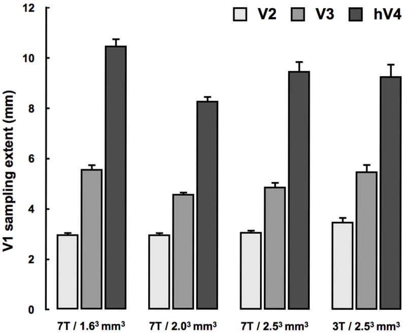
Estimates of the V1 sampling extent for three different voxel sizes and two different field-strengths for visual areas V2-hV4 in subject S1. Increasing the voxel size from 1.63 mm3 to 2.53 mm3 and then decreasing the magnetic field-strength from 7T to 3T reveals that the connective field modeling method is robust to changing these instrumental parameters; there is noise but no bias. Error-bars indicate the 95% bootstrapped confidence intervals.
DISCUSSION
Just as the receptive field of a visual neuron describes its response as a function of visual field position, the connective field of a neuron predicts its response as a function of activity in another part of the brain. Here, we have shown how fMRI can be used to estimate the connective field of a population of neurons. The analysis is based on a model of neuronal responses, accurately traces the fine-grained topographic connectivity between visual areas, and provides a quantitative estimate of the connective field size. The method is non-invasive and robust to changes in fMRI resolution as well as field-strength.
Connective field modeling represents a fundamental departure from the existing approaches to estimating fMRI connectivity in the human brain. One reason is that it emphasizes the spatial profile of the functional connectivity between brain areas: connective field modeling harnesses the core strengths of fMRI – a large field of view and high spatial resolution – to make inferences about the spatial coupling among brain areas. While some of the existing methods such as seed-voxel correlation mapping (Biswal et al., 1995) and independent component analysis (Arfanakis et al., 2000) are capable of producing spatial connectivity maps, these methods have not yet provided the level of spatial detail associated with connective field modeling. Another important aspect that is unique to connective field modeling is that it informs about the direction of information flow in terms of converging versus divergent connections. For example, if the connective field size for V1 ➤ V2 is larger than for V2 ➤ V1, this would indicate that visual information converges from V1 to V2. To the best of our knowledge, existing methods for fMRI connectivity analysis only deal with the question of directionality by framing cortical information processing in terms of temporal causation (Buchel and Friston 1997; Friston et al., 1995; Friston et al., 1997; Friston, Harrison, Penny 2003; Goebel et al., 2003; Harrison, Penny, Friston 2003), which is not a trivial thing to do with fMRI due to its poor temporal resolution.
The connective field modeling method depends on some but not all of the unwanted factors that also influence the conventional pRF estimate (Dumoulin and Wandell 2008; Smith et al., 2004). Common factors include eye and head movements, brain pulsations, and BOLD spread. These factors create a bias towards larger connective field size estimates, and add noise but no bias towards the connective field location estimates (Levin et al., 2010). Also like the pRF estimate, the connective field estimate is a statistical summary of the neuronal properties within the sampled voxel. Therefore, the connective field model parameters depend on the size and intrinsic properties of the sampled neuronal population. Different neuronal populations, for example in different cortical layers, will likely have different connective fields (Ress et al., 2007). Finally, pRF fits extending outside the maximum stimulus radius get noisy because they are based on less information than the fits that lie entirely within the stimulus area. The same is true of connective fields. If connective fields extended beyond the stimulated area of V1, then part of the connective field would be determined by the activity of the unstimulated part of V1. This unstimulated part will have lower amplitude responses than the stimulated area, so estimates here will be noisier; connective field model solutions will generally not be great for voxels near the edge of the stimulus representation.
In the present implementation of the analysis, we used a single circular symmetric, two-dimensional Gaussian connective field model. This model provides a compact description of the connective field using only two parameters. Other models, however, may also be used. The single isotropic Gaussian connective field model could be readily replaced with sums and differences of Gaussians, an anisotropic Gaussian, or any other type of mathematical function to describe the connective field. Such models may be suitable to examine connective fields in other topographically organized cortices. In addition, determining what connective field forms best explain the fMRI time-series in the different visual areas could be a very fruitful approach for understanding the different types of computation across the visual pathways.
While different stimuli may alter the connective field estimate, an important feature of connective field modeling is that the analysis itself is stimulus-independent. Consequently, the connective field models also capture some of the spontaneous signal fluctuations during periods when there is no stimulus. Using connective field modeling, therefore, it should also be possible to extract the intrinsic properties of sensory information processing based on resting-state fMRI. This idea is supported by Heinzle and colleagues’ work, who showed that “non-invasive imaging techniques such as fMRI are applicable to study detailed spatial interactions between topographically organized cortical regions in humans even in the absence of inputs driving the system under investigation” (Heinzle, Kahnt, Haynes 2011). It should be noted, however, that if connective field modeling were applied to resting-state rather than task-evoked responses, it would be important to adopt a physiological noise removal strategy, such as for example, global signal regression (Birn et al., 2006), retroicor (Glover, Li, Ress 2000), or drifter (Sarkka et al., 2012).
In conclusion, we have described and validated connective field modeling, a new model-based fMRI data-analysis that can be used to make inferences about how the spatial coupling among retinotopically organized brain regions is influenced by changes in experimental context, development, ageing, and disease. An important methodological difference between this and previous work is the use of a two-dimensional circular symmetric Gaussian connective field model. This is a valuable improvement because it is more interpretable biologically, and it allows for calculations on straightforward parameters such as the connective field size, a measure of spatial integration. Because the method is stimulus-agnostic, it should also be possible to employ the method to non-visual topographically organized brain regions as well as resting-state responses.
Acknowledgments
KVH and FWC were supported by a grant from Stichting Nederlands Oogheelkundig Onderzoek (SNOO) and European Union Grants #043157 (Syntex) and #043261 (Percept). KVH was also supported by the Groningen Research School for Behavioral and Cognitive Neurosciences (BCN) and The Netherlands Society for Biophysics and Biomedical Engineering (VVB-BMT). FWC and SOD were supported by The Netherlands Organization for Scientific Research (NWO grant #433-09-251). The software is freely available and will be distributed as part of the VISTA software package (http://white.stanford.edu/software/).
Footnotes
Publisher's Disclaimer: This is a PDF file of an unedited manuscript that has been accepted for publication. As a service to our customers we are providing this early version of the manuscript. The manuscript will undergo copyediting, typesetting, and review of the resulting proof before it is published in its final citable form. Please note that during the production process errors may be discovered which could affect the content, and all legal disclaimers that apply to the journal pertain.
References
- Amano K, Wandell BA, Dumoulin SO. Visual field maps, population receptive field sizes, and visual field coverage in the human MT+ complex. Journal of Neurophysiology. 2009;102(5):2704–2718. doi: 10.1152/jn.00102.2009. [DOI] [PMC free article] [PubMed] [Google Scholar]
- Andrews TJ, Halpern SD, Purves D. Correlated size variations in human visual cortex, lateral geniculate nucleus, and optic tract. The Journal of Neuroscience : The Official Journal of the Society for Neuroscience. 1997;17(8):2859–2868. doi: 10.1523/JNEUROSCI.17-08-02859.1997. [DOI] [PMC free article] [PubMed] [Google Scholar]
- Angelucci A, Levitt JB, Walton EJ, Hupe JM, Bullier J, Lund JS. Circuits for local and global signal integration in primary visual cortex. The Journal of Neuroscience : The Official Journal of the Society for Neuroscience. 2002;22(19):8633–8646. doi: 10.1523/JNEUROSCI.22-19-08633.2002. [DOI] [PMC free article] [PubMed] [Google Scholar]
- Arfanakis K, Cordes D, Haughton VM, Moritz CH, Quigley MA, Meyerand ME. Combining independent component analysis and correlation analysis to probe interregional connectivity in fMRI task activation datasets. Magnetic Resonance Imaging. 2000;18(8):921–930. doi: 10.1016/s0730-725x(00)00190-9. [DOI] [PubMed] [Google Scholar]
- Bandettini PA, Jesmanowicz A, Wong EC, Hyde JS. Processing strategies for time-course data sets in functional MRI of the human brain. Magnetic Resonance in Medicine : Official Journal of the Society of Magnetic Resonance in Medicine / Society of Magnetic Resonance in Medicine. 1993;30(2):161–173. doi: 10.1002/mrm.1910300204. [DOI] [PubMed] [Google Scholar]
- Baseler HA, Gouws A, Haak KV, Racey C, Crossland MD, Tufail A, Rubin GS, Cornelissen FW, Morland AB. Large-scale remapping of visual cortex is absent in adult humans with macular degeneration. Nature Neuroscience. 2011;14(5):649–655. doi: 10.1038/nn.2793. [DOI] [PubMed] [Google Scholar]
- Behrens P. CircStat: A MATLAB toolbox for circular statistics. Journal of Statistical Software. 2009;31(10):1–21. [Google Scholar]
- Birn RM, Diamond JB, Smith MA, Bandettini PA. Separating respiratory-variation-related fluctuations from neuronal-activity-related fluctuations in fMRI. NeuroImage. 2006;31(4):1536–1548. doi: 10.1016/j.neuroimage.2006.02.048. [DOI] [PubMed] [Google Scholar]
- Biswal B, Yetkin FZ, Haughton VM, Hyde JS. Functional connectivity in the motor cortex of resting human brain using echo-planar MRI. Magnetic Resonance in Medicine : Official Journal of the Society of Magnetic Resonance in Medicine / Society of Magnetic Resonance in Medicine. 1995;34(4):537–541. doi: 10.1002/mrm.1910340409. [DOI] [PubMed] [Google Scholar]
- Brainard DH. The psychophysics toolbox. Spatial Vision. 1997;10(4):433–436. [PubMed] [Google Scholar]
- Brewer AA, Liu J, Wade AR, Wandell BA. Visual field maps and stimulus selectivity in human ventral occipital cortex. Nature Neuroscience. 2005;8(8):1102–1109. doi: 10.1038/nn1507. [DOI] [PubMed] [Google Scholar]
- Buchel C, Friston KJ. Modulation of connectivity in visual pathways by attention: Cortical interactions evaluated with structural equation modelling and fMRI. Cerebral Cortex (New York, N Y : 1991) 1997;7(8):768–778. doi: 10.1093/cercor/7.8.768. [DOI] [PubMed] [Google Scholar]
- Dijkstra EW. A note on two problems in connexion with graphs. Numerische Mathematik. 1959;1(1):269–271. [Google Scholar]
- Dougherty RF, Koch VM, Brewer AA, Fischer B, Modersitzki J, Wandell BA. Visual field representations and locations of visual areas V1/2/3 in human visual cortex. Journal of Vision. 2003;3(10):586–598. doi: 10.1167/3.10.1. [DOI] [PubMed] [Google Scholar]
- Dumoulin SO, Wandell BA. Population receptive field estimates in human visual cortex. NeuroImage. 2008;39(2):647–660. doi: 10.1016/j.neuroimage.2007.09.034. [DOI] [PMC free article] [PubMed] [Google Scholar]
- Fletcher R, Powell MJD. A rapidly convergent descent method for minimization. The Computer Journal. 1963;6(2):163–168. [Google Scholar]
- Friston KJ, Harrison L, Penny W. Dynamic causal modelling. NeuroImage. 2003;19(4):1273–1302. doi: 10.1016/s1053-8119(03)00202-7. [DOI] [PubMed] [Google Scholar]
- Friston KJ, Ungerleider LG, Jezzard P, Turner R. Characterizing modulatory interactions between V1 and V2 in human cortex with fMRI. Human Brain Mapping. 1995;2:211–224. [Google Scholar]
- Friston KJ, Buechel C, Fink GR, Morris J, Rolls E, Dolan RJ. Psychophysiological and modulatory interactions in neuroimaging. NeuroImage. 1997;6(3):218–229. doi: 10.1006/nimg.1997.0291. [DOI] [PubMed] [Google Scholar]
- Gattass R, Sousa AP, Gross CG. Visuotopic organization and extent of V3 and V4 of the macaque. The Journal of Neuroscience : The Official Journal of the Society for Neuroscience. 1988;8(6):1831–1845. doi: 10.1523/JNEUROSCI.08-06-01831.1988. [DOI] [PMC free article] [PubMed] [Google Scholar]
- Gattass R, Gross CG, Sandell JH. Visual topography of V2 in the macaque. The Journal of Comparative Neurology. 1981;201(4):519–539. doi: 10.1002/cne.902010405. [DOI] [PubMed] [Google Scholar]
- Glover GH, Li TQ, Ress D. Image-based method for retrospective correction of physiological motion effects in fMRI: RETROICOR. Magnetic Resonance in Medicine : Official Journal of the Society of Magnetic Resonance in Medicine / Society of Magnetic Resonance in Medicine. 2000;44(1):162–167. doi: 10.1002/1522-2594(200007)44:1<162::aid-mrm23>3.0.co;2-e. [DOI] [PubMed] [Google Scholar]
- Goebel R, Roebroeck A, Kim DS, Formisano E. Investigating directed cortical interactions in time-resolved fMRI data using vector autoregressive modeling and granger causality mapping. Magnetic Resonance Imaging. 2003;21(10):1251–1261. doi: 10.1016/j.mri.2003.08.026. [DOI] [PubMed] [Google Scholar]
- Haak KV, Cornelissen FW, Morland AB. Population receptive field dynamics in human visual cortex. PloS One. 2012;7(5):e37686. doi: 10.1371/journal.pone.0037686. [DOI] [PMC free article] [PubMed] [Google Scholar]
- Harrison L, Penny WD, Friston K. Multivariate autoregressive modeling of fMRI time series. NeuroImage. 2003;19(4):1477–1491. doi: 10.1016/s1053-8119(03)00160-5. [DOI] [PubMed] [Google Scholar]
- Harvey BM, Dumoulin SO. The relationship between cortical magnification factor and population receptive field size in human visual cortex: Constancies in cortical architecture. The Journal of Neuroscience : The Official Journal of the Society for Neuroscience. 2011;31(38):13604–13612. doi: 10.1523/JNEUROSCI.2572-11.2011. [DOI] [PMC free article] [PubMed] [Google Scholar]
- Heinzle J, Kahnt T, Haynes JD. Topographically specific functional connectivity between visual field maps in the human brain. NeuroImage. 2011;56(3):1426–1436. doi: 10.1016/j.neuroimage.2011.02.077. [DOI] [PubMed] [Google Scholar]
- Jammalamadaka SR, Sengupta A. Topics in circular statistics. World Scientific 2001 [Google Scholar]
- Kumano H, Uka T. The spatial profile of macaque MT neurons is consistent with gaussian sampling of logarithmically coordinated visual representation. Journal of Neurophysiology. 2010;104(1):61–75. doi: 10.1152/jn.00040.2010. [DOI] [PubMed] [Google Scholar]
- Lehky SR, Sejnowski TJ. Network model of shape-from-shading: Neural function arises from both receptive and projective fields. Nature. 1988;333(6172):452–454. doi: 10.1038/333452a0. [DOI] [PubMed] [Google Scholar]
- Levin N, Dumoulin SO, Winawer J, Dougherty RF, Wandell BA. Cortical maps and white matter tracts following long period of visual deprivation and retinal image restoration. Neuron. 2010;65(1):21–31. doi: 10.1016/j.neuron.2009.12.006. [DOI] [PMC free article] [PubMed] [Google Scholar]
- Logothetis NK. What we can do and what we cannot do with fMRI. Nature. 2008;453(7197):869–878. doi: 10.1038/nature06976. [DOI] [PubMed] [Google Scholar]
- Motter BC. Central V4 receptive fields are scaled by the V1 cortical magnification and correspond to a constant-sized sampling of the V1 surface. The Journal of Neuroscience : The Official Journal of the Society for Neuroscience. 2009;29(18):5749–5757. doi: 10.1523/JNEUROSCI.4496-08.2009. [DOI] [PMC free article] [PubMed] [Google Scholar]
- Nestares O, Heeger DJ. Robust multiresolution alignment of MRI brain volumes. Magnetic Resonance in Medicine : Official Journal of the Society of Magnetic Resonance in Medicine / Society of Magnetic Resonance in Medicine. 2000;43(5):705–715. doi: 10.1002/(sici)1522-2594(200005)43:5<705::aid-mrm13>3.0.co;2-r. [DOI] [PubMed] [Google Scholar]
- Ogawa S, Menon RS, Kim SG, Ugurbil K. On the characteristics of functional magnetic resonance imaging of the brain. Annual Review of Biophysics and Biomolecular Structure. 1998;27:447–474. doi: 10.1146/annurev.biophys.27.1.447. [DOI] [PubMed] [Google Scholar]
- Pelli DG. Crowding: A cortical constraint on object recognition. Current Opinion in Neurobiology. 2008;18(4):445–451. doi: 10.1016/j.conb.2008.09.008. [DOI] [PMC free article] [PubMed] [Google Scholar]
- Pelli DG. The VideoToolbox software for visual psychophysics: Transforming numbers into movies. Spatial Vision. 1997;10(4):437–442. [PubMed] [Google Scholar]
- Pelli DG, Tillman KA. The uncrowded window of object recognition. Nature Neuroscience. 2008;11(10):1129–1135. doi: 10.1038/nn.2187. [DOI] [PMC free article] [PubMed] [Google Scholar]
- Ress D, Glover GH, Liu J, Wandell B. Laminar profiles of functional activity in the human brain. NeuroImage. 2007;34(1):74–84. doi: 10.1016/j.neuroimage.2006.08.020. [DOI] [PubMed] [Google Scholar]
- Salin PA, Bullier J. Corticocortical connections in the visual system: Structure and function. Physiological Reviews. 1995;75(1):107–154. doi: 10.1152/physrev.1995.75.1.107. [DOI] [PubMed] [Google Scholar]
- Sarkka S, Solin A, Nummenmaa A, Vehtari A, Auranen T, Vanni S, Lin FH. Dynamic retrospective filtering of physiological noise in BOLD fMRI: DRIFTER. NeuroImage. 2012;60(2):1517–1527. doi: 10.1016/j.neuroimage.2012.01.067. [DOI] [PMC free article] [PubMed] [Google Scholar]
- Schwarzkopf DS, Song C, Rees G. The surface area of human V1 predicts the subjective experience of object size. Nature Neuroscience. 2011;14(1):28–30. doi: 10.1038/nn.2706. [DOI] [PMC free article] [PubMed] [Google Scholar]
- Sholl DA. Dendritic organization in the neurons of the visual and motor cortices of the cat. Journal of Anatomy. 1953;87(4):387–406. [PMC free article] [PubMed] [Google Scholar]
- Smith SM, Jenkinson M, Woolrich MW, Beckmann CF, Behrens TE, Johansen-Berg H, Bannister PR, De Luca M, Drobnjak I, Flitney DE, et al. Advances in functional and structural MR image analysis and implementation as FSL. NeuroImage. 2004;23(Suppl 1):S208–19. doi: 10.1016/j.neuroimage.2004.07.051. [DOI] [PubMed] [Google Scholar]
- Teo PC, Sapiro G, Wandell BA. Creating connected representations of cortical gray matter for functional MRI visualization. IEEE Transactions on Medical Imaging. 1997;16(6):852–863. doi: 10.1109/42.650881. [DOI] [PubMed] [Google Scholar]
- Tootell RB, Mendola JD, Hadjikhani NK, Liu AK, Dale AM. The representation of the ipsilateral visual field in human cerebral cortex. Proceedings of the National Academy of Sciences of the United States of America. 1998;95(3):818–824. doi: 10.1073/pnas.95.3.818. [DOI] [PMC free article] [PubMed] [Google Scholar]
- Wandell BA, Winawer J. Imaging retinotopic maps in the human brain. Vision Research. 2011;51(7):718–737. doi: 10.1016/j.visres.2010.08.004. [DOI] [PMC free article] [PubMed] [Google Scholar]
- Wandell BA, Dumoulin SO, Brewer AA. Visual field maps in human cortex. Neuron. 2007;56(2):366–383. doi: 10.1016/j.neuron.2007.10.012. [DOI] [PubMed] [Google Scholar]
- Wandell BA, Chial S, Backus BT. Visualization and measurement of the cortical surface. Journal of Cognitive Neuroscience. 2000;12(5):739–752. doi: 10.1162/089892900562561. [DOI] [PubMed] [Google Scholar]
- Winawer J, Horiguchi H, Sayres RA, Amano K, Wandell BA. Mapping hV4 and ventral occipital cortex: The venous eclipse. Journal of Vision. 2010;10(5):1. doi: 10.1167/10.5.1. [DOI] [PMC free article] [PubMed] [Google Scholar]
- Zuiderbaan W, Harvey BM, Dumoulin SO. Modeling center-surround configurations in population receptive fields using fMRI. Journal of Vision. 2012;12(3) doi: 10.1167/12.3.10. Print 2012. [DOI] [PubMed] [Google Scholar]