Test for interactions between a genetic marker set and environment in generalized linear models

Abstract

We consider in this paper testing for interactions between a genetic marker set and an environmental variable. A common practice in studying gene–environment (GE) interactions is to analyze one single-nucleotide polymorphism (SNP) at a time. It is of significant interest to analyze SNPs in a biologically defined set simultaneously, e.g. gene or pathway. In this paper, we first show that if the main effects of multiple SNPs in a set are associated with a disease/trait, the classical single SNP–GE interaction analysis can be biased. We derive the asymptotic bias and study the conditions under which the classical single SNP–GE interaction analysis is unbiased. We further show that, the simple minimum p-value-based SNP-set GE analysis, can be biased and have an inflated Type 1 error rate. To overcome these difficulties, we propose a computationally efficient and powerful gene–environment set association test (GESAT) in generalized linear models. Our method tests for SNP-set by environment interactions using a variance component test, and estimates the main SNP effects under the null hypothesis using ridge regression. We evaluate the performance of GESAT using simulation studies, and apply GESAT to data from the Harvard lung cancer genetic study to investigate GE interactions between the SNPs in the 15q24–25.1 region and smoking on lung cancer risk.

1. Introduction

Complex diseases are often caused by the interplay of genes and environment. For example, exposure to an environmental factor increases disease risk only for patients with specific genetic profiles; patients with certain genetic profiles have increased disease risk only if they are exposed to an environment. Identification of gene–environment (GE) interactions has important implications for understanding underlying disease etiology and developing disease prevention and intervention strategies. Genome-wide association studies (GWAS), wherein a large number of single-nucleotide polymorphisms (SNPs) are genotyped, provide a rich opportunity to study GE interactions besides identifying genetic loci that are associated with diseases/traits. We consider in this paper testing for the interaction effects between multiple SNPs in an SNP-set and an environmental variable on outcomes.

The work in this paper is motivated by a problem to identify GE interaction effects on lung cancer risk. The 15q24–25.1 region contains several biologically interesting genes for lung cancer and nicotine addiction. The published GWAS studies identified several variants in this region that are associated with both lung cancer risk and smoking behavior (see Hung and others, 2008; Furberg and others, 2010, for example). The Harvard lung cancer case–control study consists of 1941 subjects (980 lung cancer cases and 961 controls). Smoking variables and genotypes of 26 SNPs in the 15q24–25.1 region are available. A question of major interest is to study whether the increased lung cancer risk associated with the multiple variants in this region is modified by smoking status. In other words, we are interested in examining the interaction effects between the 15q24–25.1 region, which consists of multiple SNPs and smoking on lung cancer risk.

In a typical GWAS, GE interactions are investigated by testing the interaction of each SNP and an environmental variable separately, and then adjusted for multiple testing across the genome. Several recent efforts have been made to improve the power of the classical single-marker GE interaction test (Hsu and others, 2012) using an empirical Bayes method (Mukherjee and Chatterjee, 2008) and two-stage analysis (Murcray and others, 2011). Despite these efforts, the single-marker test has several limitations. First, multiple comparison adjustment for a large number of markers across the genome could result in power loss. Secondly, the typed SNPs, i.e. SNPs on a GWAS chip, are often correlated due to linkage disequilibrium (LD). Furthermore, multiple tests for GE interactions in these single-marker-based GE interaction models are even more dependent, as interaction terms in these models share the same environmental variable. Dependence among multiple tests can result in incorrect Type 1 error rates and causes bias in standard multiple comparison adjustments, such as the Bonferroni method, and this bias is often difficult to correct. Third, the single-marker GE test does not interrogate the joint effects of multiple SNPs that have similar biological functions. Moreover, as we will show, when there are multiple SNPs whose main effects are associated with a disease/trait, the single-marker GE test misspecifies the null model and may result in inflated Type 1 error in testing for GE interactions.

There has been interest in multiple marker analysis by grouping SNPs into biological meaningful SNP-sets, e.g. SNPs in a gene, haplotype block, or pathway, to improve analysis power and results interpretability. See Wu and others (2010) for detailed discussions of forming SNP-sets. The existing SNP-set analysis has focused on testing for the main effects of an SNP-set (Tzeng and Zhang, 2007; Wu and others, 2010). Limited work has been done on testing for the interactions between a marker set and an environmental variable. Tzeng and others (2011) developed a test for the interactions between a marker set and an environmental variable for continuous traits by regressing the similarity matrix of a continuous outcome on the similarity matrix of SNPs in a set. However, this approach is difficult to extend to non-Gaussian traits, such as a binary trait, because of the complex constraints of the similarity matrix of binary traits.

This paper has two objectives. First, we investigate the asymptotic bias of the single-marker GE interaction test, and show that when multiple SNPs within an SNP-set are associated with a disease/trait in their main effects, the single-marker GE interaction test is generally biased. As a consequence, we show that the simple SNP-set GE interaction analysis using the minimum of the single-marker GE interaction p-values (min test), can be biased and may be subjected to inflated Type 1 error rates. Secondly, to overcome these difficulties, we propose a powerful and computationally efficient test called gene–environment set association test (GESAT), for assessing the interaction effects of a set of markers and an environmental variable for continuous and discrete outcomes. Specifically, we assume the coefficients of the GE interaction terms to be random effects, and develop a variance component score test within the induced generalized linear mixed model (GLMM) framework. As some SNPs in a set are likely to be highly correlated due to high LD, we use ridge regression to estimate the SNP main effects under the null model.

The remainder of the paper is organized as follows. In Section 2, we introduce the SNP-set GE interaction model. In Section 3, we investigate the asymptotic bias of the single-marker GE interaction test. In Section 4, we describe the GESAT testing procedure. In Section 5, we evaluate the finite sample performance of GESAT using simulations. In Section 6, we apply GESAT to the Harvard lung cancer data to study the interaction effects of the 15q24–25.1 region and smoking on lung cancer risk. We conclude with discussions in Section 7.

2. Marker set and environmental interaction generalized linear models

Suppose that the data consist of n independent and identically distributed random vectors for i=1,…,n, where Y _i is the phenotype of the ith sample, and , X_i=(X_i1,…,X_iq)^T is a vector of q non-genetic covariates, and E_i is a scalar environmental variable, and G_i=(G_i1,…,G_ip)^T is a vector of p genetic markers, which form a SNP-set. Without loss of generality, we consider a scalar environmental variable E. Define S_i=(E_iG_i1,…,E_iG_ip)^T to be a vector of GE interaction terms for the ith individual. Suppose conditional on , Y _i follows a distribution in the exponential family (McCullagh and Nelder, 1989) where f(⋅) is the density of , and a(⋅), b(⋅), and c(⋅) are some known functions, and θ_i and ϕ are the canonical parameter and the dispersion parameter, respectively. Denote by . We consider the following marker-set and environment interaction GLM (McCullagh and Nelder, 1989)

(2.1)

where g(⋅) is a monotone link function. For simplicity, we assume g(⋅) is a canonical link function. Define an n×1 environmental variable vector E=(E₁,…,E_n)^T, an n×q covariate matrix X=[X₁…X_n]^T, an n×p genotype matrix G=[G₁…G_n]^T and an n×p GE interaction matrix S=[S₁…S_n]^T. In matrix notation, model (2.1) can be written as

(2.2)

where μ=(μ₁,…,μ_n)^T, , and . We are interested in testing if there is a marker set and environment interaction, i.e. H₀:β=0.

3. Asymptotic bias analysis of the single-marker gene–environment test

A common approach for studying GE interactions is to analyze one SNP at a time. In this section, we study the asymptotic bias of the maximum-likelihood estimator (MLE) of the GE interaction coefficient in the classical single-marker GE interaction model, when multiple SNPs are associated with the outcome. We show that the single-maker-based GE interaction test is generally biased and may result in an inflated Type 1 error rate.

3.1. Analytic asymptotic bias of the single-marker gene–environment test

For simplicity, in our asymptotic bias analysis, we assume no covariates are present. Suppose the data are generated from the following multi-maker GE interaction model

(3.1)

The single-marker GE interaction test assumes the following misspecified model using only the jth genetic marker (j=1,…,p)

(3.2)

Simple calculations show the score equation for estimating under (3.2) is

(3.3)

where μ(⋅)=g⁻¹(⋅). The asymptotic limit of the score equation (3.3) is given by

(3.4)

where and , and the expectation is taken under the true model (3.1). The MLEs calculated under the misspecified single-marker GE interaction model (3.2), , solve the misspecified score equation (3.3). It is easy to show that the asymptotic limits of the MLEs, , can be obtained by solving equation (3.4).

The closed-form expressions of are generally not available, and are generally not equal to the true values (α₁,α₂,α_3j,β_j). Indeed, under the null hypothesis of no interaction between the marker set G and environment E in the true multi-marker model, i.e. H₀:β=0 in model (3.1), one can show that is generally not 0. This means if the true outcome model is a multi-marker model, the single-marker GE interaction test is generally biased and does not have a correct Type 1 error rate.

Consequently to test the null hypothesis of no SNP-set by environmental interactions, i.e. H₀:β=0 under the multi-marker GE interaction model (3.1), the min test will generally be invalid and has an incorrect Type 1 error rate. Specifically, to test H₀:β=0, the min test calculates the p-value for testing in the single-marker GE model (3.2) for each marker j, and adjusts the minimum of these p-values accounting for multiple testing. As each p-value is generally biased, the minimum of them is biased as well.

In some special cases, we can derive closed-form expressions of the asymptotic limits . Specifically, when g(⋅) is an identity link function and G and E are all binary, we can calculate the explicit expressions of these asymptotic limits. Define . In Section A.1 (supplementary material available at Biostatistics online), we show that the asymptotic limits of the MLEs under the misspecified single-marker GE interaction model (3.2), which are the solutions of Equation (3.4) are

(3.5)

The asymptotic bias of is given by . In general, will not be the same as β_j, and so will be asymptotically biased.

It is of significant interest to identify situations where the GE interaction coefficient using the single-marker GE interaction model (3.2) is unbiased when the true model is the multi-marker GE interaction model (3.1). One trivial case is when α_3k=β_k=0 for all k≠j. For the identity link function, from Equations (3.5), it is straightforward to show that under the null hypothesis H₀:β=0 in the multi-marker GE interaction model (3.1), if (i) (G_j,E) is independent of {G_k}_k≠j or (ii) G_j is independent of (E,{G_k}_k≠j) or (iii) is independent of E, we have that . This means, under (i)–(iii), the single-marker GE interaction coefficient estimator is asymptotically unbiased under the null. VanderWeele and others (2012) obtained similar findings in GE interaction models in the presence of unmeasured confounders using the causal inference method. We note, however, that even if the single-marker GE interaction coefficient estimator is asymptotically unbiased under the null, standard inference can still be wrong as the conventional standard error estimate can be biased (Section A.2, supplementary material available at Biostatistics online).

3.2. Numerical examples of asymptotic bias analysis

Consider linear regression with two SNPs (p=2). Suppose the true model is

and the misspecified single-marker GE model using G₁ is

Suppose the two SNPs, G₁ and G₂, are independent. Let MAF₁ and MAF₂ be their minor allele frequencies (MAFs). Assuming a dominant model, we have G₁∼Binom{1,1−(1−MAF₁)²} and G₂∼Binom{1,1−(1−MAF₂)²}. Suppose a binary environmental variable E is related to the genotypes G₁ and G₂ through the logistic model

(3.6)

Then the asymptotic limit of can be calculated using Equations (3.5) and (3.6).

Besides the trivial case where α₃₂=β₂=0, we first note that there are three distinct scenarios where has no asymptotic bias for all values of α₃₂ and β₂ since we assume G₁ and G₂ are independent: (i) G₁ independent of E (i.e. ρ₁=ρ₃=0), (ii) G₂ independent of E (i.e. ρ₂=ρ₃=0), and (iii) G₁,G₂,E independent (i.e. ρ₁=ρ₂=ρ₃=0).

We conducted numerical studies to investigate the asymptotic bias of in a number of different scenarios. We assumed MAF₁=0.2,MAF₂=0.3,α₁=0,α₂=0.4. Besides computing the theoretical asymptotic bias using Equation (3.5), we also simulated data with sample size n=1000 and calculated the empirical bias obtained by averaging over 5000 simulations.

We first considered the case where the null hypothesis holds, i.e. β₁=β₂=0. In the top panel of Table 1, we set α₃₁=α₃₂=ρ₁=ρ₂=ρ₃ and varied these values from 0 to 1 in steps of 0.10. This corresponds to the case where the environmental factor is positively associated with the SNPs, and increase in environmental factor and/or SNPs corresponds to an increase in the mean of the outcome. In this scenario, the bias is always positive, that is . In bottom panel of Table 1, we set α₃₁=α₃₂=−ρ₁=−ρ₂=−ρ₃ and varied these values from 0 to 1 in steps of 0.10. This corresponds to the case where the environmental factor is negatively associated with the SNPs, and an increase in environmental factor and/or SNPs corresponds to an increase in the mean of the outcome. In this scenario, the bias is always negative, that is, . These results make sense intuitively, as the misspecified single-marker GE model omits G₂. Thus when E and G₂ are positively associated, we expect to have the same sign as α₃₂, the regression coefficient of G₂ in the true model. When E and G₂ are negatively associated, we expect the sign of to be opposite that of α₃₂. As expected, since is biased asymptotically, the Wald test based on has an inflated Type 1 error rate (last column of Table 1).

Table 1.

Asymptotic and empirical biases of under the null hypothesis of no interaction between a marker set and environment, and inflated Type 1 error rates at α=0.05 level when (G₁,G₂) and E are not independent

α31=α32=ρ1=ρ2=ρ3	Empirical	Theoretical	Empirical Type 1 error
0.00	0.003	0.000	0.047
0.10	0.002	0.002	0.052
0.20	0.010	0.010	0.051
0.30	0.022	0.022	0.053
0.40	0.037	0.039	0.059
0.50	0.058	0.059	0.065
0.60	0.083	0.082	0.079
0.70	0.106	0.107	0.098
0.80	0.126	0.132	0.113
0.90	0.156	0.155	0.139
1.00	0.173	0.176	0.146
α31=α32=−ρ1=−ρ2=−ρ3	Empirical	Theoretical	Empirical Type 1 error
0.00	−0.001	0.000	0.045
0.10	−0.006	−0.002	0.049
0.20	−0.012	−0.010	0.051
0.30	−0.024	−0.022	0.050
0.40	−0.035	−0.039	0.062
0.50	−0.057	−0.059	0.066
0.60	−0.081	−0.082	0.081
0.70	−0.104	−0.107	0.107
0.80	−0.134	−0.132	0.122
0.90	−0.157	−0.155	0.133
1.00	−0.178	−0.176	0.161

We next considered the case of the alternative hypothesis, i.e. β₁=β₂≠0. In the left panel of Figure 1, we set α₃₁=α₃₂=β₁=β₂=ρ₁=ρ₂=ρ₃. In the right panel of Figure 1, we set α₃₁=α₃₂=β₁=β₂=−ρ₁=−ρ₂=−ρ₃. We varied β₁ from 0 to 1 in steps of 0.05. The bias is always positive in the first case while the bias is always negative in the second case , for the same reason given above.

Figure 1.

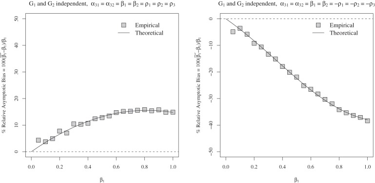
Asymptotic and empirical biases of the interaction coefficient under the single-marker GE interaction model (3.2) when (G₁,G₂) and E are not independent. The horizontal axis gives true β₁ under the true multi-marker GE interaction model (3.1), and the vertical axis gives the percentage of the relative bias in estimating β₁. % Relative asymptotic bias is computed as . Left panel: α₃₁= α₃₂=β₁=β₂=ρ₁=ρ₂=ρ₃. Right panel: α₃₁=α₃₂=β₁=β₂=−ρ₁=−ρ₂=−ρ₃. Square gives the empirical % relative bias by averaging over 5000 simulations for sample size n=1000. Solid line gives the theoretical % relative asymptotic bias computed using the closed-form expressions for in (3.5).

In our data example, the 26 SNPs in the 15q24–25.1 region may be associated with both lung cancer risk (phenotype) and smoking (environmental factor) since genes in this region have been implicated in both lung cancer risk and nicotine dependence. Thus, if more than one SNP in this region are associated with smoking and have main effects, using a single-marker test to assess SNP-smoking interaction may be inadequate. In the remainder of this paper, we develop GESAT, a SNP-set—environment interaction statistical framework—which allows us to adjust for the main effects of all SNPs while simultaneously testing for the interactions between the SNPs in the region and smoking on lung cancer risk.

4. Gene–environment set association test

4.1. Derivation of the test statistic

We consider in this section testing H₀:β=0 under the multi-marker GE interaction model (2.1). A classical approach treats β_j’s as fixed effects and proceeds with a p degrees of freedom (DF) test. This approach can suffer from power loss when p is moderate/large, and numerical difficulties when some genetic markers in the set are in high LD.

To overcome this problem, we derive a test statistic for testing H₀ by assuming β_j’s follow an arbitrary distribution with mean zero and common variance τ² and that the β_j’s are independent. The GE interaction GLM (2.1) then becomes a GLMM (Breslow and Clayton, 1993). The null hypothesis H₀:β=0 is then equivalent to H₀:τ²=0. We hence can perform a variance component test using a score test under the induced GLMM. This approach allows one to borrow information among the β_j’s. The variance component score test has two advantages: first, it is locally most powerful under some regularity conditions (Lin, 1997); secondly, it requires only fitting the model under the null hypothesis and is computationally attractive.

Following Lin, 1997, the score statistic for the variance component τ is

(4.1)

where and is estimated under the null main effects model,

(4.2)

If the dimension of α is small, one can use regular maximum likelihood to estimate α. However, because the number of SNPs p in a set is likely to be large and some SNPs might be in high LD with each other, the regular MLE might not be stable or difficult to calculate. We propose using ridge regression to estimate α under the null model (4.2), where we impose a L₂ penalty on the coefficients of the main SNP effects α₃. The penalized log-likelihood under the null model (4.2) is where , f(⋅) is the density of Y _i under the null model (4.2) and λ is a tuning parameter.

Given λ, simple calculations show that estimation of α under the null model (4.2) proceeds by solving the estimating equation where I₂ is (q+1+p)×(q+1+p) block diagonal matrix with the top (q+1)×(q+1) block diagonal matrix being 0 and the bottom p×p block diagonal matrix being an identity matrix I_p×p.

4.2. Evaluation of the null distribution of the test statistic

Under main effect models, Zhang and Lin (2003) and Wu and others (2010) showed that the null distribution of the variance component score test follows a mixture of χ² distribution asymptotically. However, our score test statistic Q in Equation (4.1) is different from their test statistic, since we use ridge regression to estimate α under the null model. In this section, we derive the null distribution of the test statistic Q, and show that it follows a mixture of χ² distribution with different mixing coefficients that depend on the tuning parameter λ.

Suppose the estimated tuning parameter . Define where Δ=diag{g′(μ_i)}, and let α₀ and Δ₀ be the true value of α and Δ under H₀. In Section B.1 (supplementary material available at Biostatistics online), we show that under H₀, we have

(4.3)

where , , , and , which is the GLM working vector. Define

then the null distribution of Q is approximately equals to , where d_v is the vth eigenvalue of the matrix Σ^1/2Δ₀AΔ₀Σ^1/2, and s are iid χ² random variables with 1 DF. The p-value of the test statistic Q can then be obtained using the characteristic function inversion method (Davies, 1980). In Section B.2 (supplementary material available at Biostatistics online), we describe how the tuning parameter λ is selected using generalized cross validation (O’Sullivan and others, 1986).

5. Simulation studies

We conducted simulations to evaluate the finite sample performance of GESAT. We simulated 166 HapMap SNPs in the 15q24–25.1 region using the LD structure of the CEU population in the HapMap project. To mimic the Harvard lung cancer data, only the 26 typed variants on Illumina 610-Quad array in this region are used for analysis. These 26 typed SNPs form the SNP-set used for analysis in simulations and the data example in Section 6. We restricted the analysis to common variants (MAF ≥0.05), giving p=25−26. Based on LD structure in the region, we selected a group of 5 candidate untyped SNPs from which the causal SNPs are chosen (Section C.2, supplementary material available at Biostatistics online). We considered the SNP-set and environment interaction model in Equation (2.1), where G contains the 26 typed SNPs in the 15q24–25.1 region. To test for the null hypothesis of no marker-set and environment interactions, we computed the min test as a benchmark, correcting the smallest p-value for multiple comparisons using the effective number of DF (Gao and others, 2008) and the Bonferroni method (Section C.1, supplementary material available at Biostatistics online).

5.1. Comparing GESAT and min test when G and E are independent

We first considered the case when G and E are independent. We report both empirical Type 1 error and power results. We generated a binary outcome assuming a logistic regression model

where , X₁ mimics age and is normally distributed with mean 62.4 and standard deviation 11.5, and X₂ mimics sex and takes on 1 and 2 with probability 0.52 and 0.48, respectively. For each dataset, SNP1 and SNP2 are randomly selected from the group of 5 candidate causal SNPs described above, independent of E. For the environmental variable E, we considered three cases: (i) a Bernoulli random variable taking 1 with probability 0.87 (mimicking the Harvard lung cancer data), (ii) a Bernoulli random variable taking 1 with probability 0.5, and (iii) a standard normal random variable. Each dataset had a sample size of n=2000 (1000 cases and 1000 controls). We generated 100 000 datasets and 500 datasets, respectively, to evaluate the empirical size and empirical power at α=0.05 level. We calculated GESAT and min test using X₁,X₂, E, and the 26 typed SNPs.

To evaluate the Type 1 error, we set β₁=β₂=0. For all the three configurations of E, the empirical Type 1 error is evaluated for two distinct scenarios: (a) α_SNP1=α_SNP2=0 and (b) α_SNP1=α_SNP2=0.4. The empirical size at the nominal Type 1 error of 0.05 is shown in Table 2, indicating that both GESAT and min test have protected Type 1 error rates. We note that the empirical Type 1 error rates of the min test can be slightly conservative.

Table 2.

Empirical Type 1 error rates for both GESAT and min test calculated using 10⁵ simulations at 0.05 level when G and E are independent

αSNP1,αSNP2	Environmental variable	GESAT	min Test
0	Bernoulli w. prob 0.87	5.05e−02	3.09e−02
0	Bernoulli w. prob 0.5	5.12e−02	3.58e−02
0	Standard Normal	5.18e−02	3.53e−02
0.4	Bernoulli w. prob 0.87	5.22e−02	3.23e−02
0.4	Bernoulli w. prob 0.5	5.15e−02	3.83e−02
0.4	Standard Normal	5.11e−02	3.58e−02

We conducted additional Type 1 error simulations (Section C.3, supplementary material available at Biostatistics online) for both the 15q24–25.1 region and the ASAH1 gene (which has stronger LD) for various sample sizes, distributions of environmental variables, MAFs of the causal variants, number of causal variants, and different Type 1 error levels. Similar results are obtained.

To calculate power, we varied β₁=β₂ from 0 to 0.6 in a step of 0.05. Likewise, for all three configurations of E, we calculated the power for two scenarios: (a) α_SNP1=α_SNP2=0 (left panel of Figure 2) and (b) α_SNP1=α_SNP2=0.4 (right panel of Figure 2). Our results show that GESAT performs well and generally outperforms min test. For unbalanced designs when a binary environmental exposure has a low frequency in one category (top panel in Figure 2), GESAT is most advantageous over min test (Figure 2), and min test is the most conservative (Table 2). Such unbalanced designs can occur due to case–control sampling and the strong association of an environmental factor with disease. For example in the Harvard lung cancer genetic study data example in Section 6, most cases and controls are ever smokers (87%), as the controls are frequency matched to cases with respect to age, sex, smoking status as part of the study design.

Figure 2.

Empirical power curves at α=0.05 level of significance for GESAT (dashed line) and min test (solid line) assuming G and E are independent. Top panel: Environmental factor is Bernoulli with probability 0.87; Middle panel: Environmental factor is Bernoulli with probability 0.5; Bottom panel: Environmental factor is standard normal. Left panel: SNPs have no main effect (α_SNP1=α_SNP2=0); Right panel: SNPs have main effects (α_SNP1=α_SNP2=0.4).

We conducted several additional simulation studies. We studied the power using imputed SNPs when there is a single genotyped causal locus for the ASAH1 gene (Section C.4, supplementary material available at Biostatistics online). This is a scenario optimized for the min test as there is only a single causal SNP. When the effect size is modest, GESAT performs better than the min test, but when the effect size is strong, the min test performs better than GESAT. We also report simulations by fitting the null model using regular regression instead of ridge regression (Section C.5, supplementary material available at Biostatistics online). The results show a non-trivial number of simulations failed to converge using the regular regression method. Also, we performed simulations by comparing GESAT with the similarity regression approach of Tzeng and others (2011) (Section C.7, supplementary material available at Biostatistics online) for continuous outcomes. The two methods yield similar results, while GESAT is much faster.

5.2. Comparing GESAT and min test when G and E are not independent

We compare in this section GESAT and min test when the environmental variable E and the genotypes G are not independent. Similar to before, we generated a binary outcome assuming

where . The non-genetic covariates (X₁,X₂), the causal genetic markers (SNP1 and SNP2) and the 26 typed SNPs used for SNP-set and environmental interaction test are obtained as before. However, now we generated the binary environmental factor E to depend on the causal SNPs as

Thus ρ₁ and ρ₂ control the association between the causal genetic markers (SNP1 and SNP2) and E. We calculated GESAT and min test using X₁,X₂, E, and the 26 typed SNPs. Since the typed SNPs are in LD with the causal genetic markers (SNP1 and SNP2), ρ₁ and ρ₂ also control the association between E and the typed SNPs used for fitting model (2.1). We examined two distinct scenarios: (a) ρ₁=ρ₂ and (b) ρ₁=−ρ₂. In all cases, we set β₁=β₂ and had sample size n=2000 (1000 cases, 1000 controls). To investigate the Type 1 error rate, we set β₁=β₂=0. To study power of GESAT, we varied β₁=β₂ from 0 to 0.6 in a step of 0.05. We varied ρ₁ to investigate how the Type 1 error rate and power depend on the association between G and E. Empirical Type 1 error and power are evaluated using 5000 and 500 simulations, respectively.

The empirical Type 1 error rate at 0.05 level for the two scenarios (a) ρ₁=ρ₂ and (b) ρ₁=−ρ₂ are plotted in the top panel of Figure 3. For (a) ρ₁=ρ₂ (left figure), we varied ρ₁ from 0 to 1 in a step of 0.05, while for (b) ρ₁=−ρ₂ (right figure), we varied ρ₁ from 0 to 2 in a step of 0.05. Note that the left and right figures in the top panel of Figure 3 have the same scale and range on the vertical axis, but not the same scale and range on the horizontal axis. In both scenarios, Type 1 error rate of min test increases with increasing ρ₁. At low values of ρ₁, the min test is conservative, while at high values of ρ₁, the Type 1 error rate is inflated. Thus as expected, when G and E are dependent, min test can have an incorrect Type 1 error rate. In comparison, GESAT maintains the nominal Type 1 error rate even when G and E are dependent.

Figure 3.

Type 1 error of GESAT is robust to the dependence of G and E but min test can give inflated Type 1 error rate—Empirical Type 1 error rates at 0.05 level for GESAT (dashed line) and min test (solid line) when G and E are dependent, are given in the top panel. In the left panel, ρ₁=ρ₂. In the right panel, ρ₁=−ρ₂. Power of GESAT is robust to association between G and E—Dashed, dotted, dashed-and-dotted lines give power of GESAT at 0.05 level when ρ₁=0,0.5,1, respectively, in the bottom panel. The models for generating the data are given in Section 5.2. The parameters ρ₁,ρ₂ control the association between G and E.

The power of GESAT for the two scenarios are plotted in the bottom panel of Figure 3. We do not report power of min test as the min test can have inflated Type 1 error rates when G and E are dependent. For each setting/figure, we used three different values of ρ₁=0,0.5,1 and varied β₁=β₂ from 0 to 0.6 in a step of 0.05. Our simulations suggest that the power of GESAT seems fairly robust to the dependence between G and E. More detailed discussions of the results can be found in Section C.6 (supplementary material available at Biostatistics online). Additional simulation results using different values of ρ₁,ρ₂ provide similar results (Section C.6, supplementary material available at Biostatistics online).

6. Application to the Harvard lung cancer genetic data

The 15q24–25.1 region was previously found to be associated with lung cancer and nicotine dependence (Hung and others, 2008; Furberg and others, 2010). This region contains many genes, including the nicotinic receptor subunit gene cluster. Initially it was unclear whether the effect of the genetic variant(s) in this region on lung cancer was restricted to smokers (Hung and others, 2008). However, subsequent studies confirmed that the lung cancer associated variant(s) identified in GWAS in this region only had an effect on lung cancer among smokers (Truong and others, 2010), suggesting a potential GE interaction.

Our study consists of Caucasian subjects drawn from a lung cancer case–control study at Massachusetts General Hospital (VanderWeele and others, 2012). There are 26 typed SNPs in the 15q24–25.1 region (Section D, supplementary material available at Biostatistics online for more details). Lung cancer case/control status, age, sex, and smoking status of the subjects are also available. We applied both GESAT and min test to study whether there is a GE interaction in this region, using smoking status (ever smokers vs. never smokers) as an environmental factor. The data analysis used 1941 samples, including 980 cases with 92 never smokers and 961 controls with 159 never smokers.

We applied GESAT to test the interaction between the SNP-set in the 15q24–25.1 region and smoking, adjusting for age, sex, smoking status, and four principal components under model (2.1), and test for H₀:β=0. Here G consists of p=26 typed SNPs in this region. GESAT gave a p-value of 0.0434, which indicates a significant interaction between the 15q24–25.1 region and smoking. For comparison, we also report results using the min test (Table S12, supplementary material available at Biostatistics online), adjusting for age, sex, smoking status, four principal components, and the main SNP effect. The min test had a p-value of 0.0103×16=0.165, which is not significant. See Section D (supplementary material available at Biostatistics online) for more details. We note also that the regular logistic regression model including the 26 SNP main effects and 26 SNP-smoking interaction terms (in addition to covariates) did not converge, thus a conventional multi-marker p DF test could not be conducted. Our results show the presence of a GE interaction in the region, i.e. the effect of variant(s) in 15q24–25.1 region on lung cancer risk is modified by smoking status.

7. Discussions

In this paper, we first studied the asymptotic bias of the traditional single genetic marker-based GE interaction test. We showed that when multiple genetic markers are associated with an outcome in their main effects, the classical single genetic marker-based GE interaction test is generally biased. As a consequence, the simple min test is generally biased. Besides power loss due to large DF, as illustrated in our data example, the traditional p DF test for testing GE interactions faces numerical difficulties due to high LD among some markers.

We proposed GESAT, a variance component score test for testing for the interactions between a genetic marker set and an environmental variable, and showed it is powerful in a wide range of settings. Unlike the existing main effect genetic marker set tests, given a possibly large number of correlated genetic markers in a set whose main effects need to be estimated under the null model, we fit the null model using ridge regression. We demonstrated via simulation studies and a real data application that our approach is robust and performs well with attractive power. GESAT is also computationally efficient, has meaningful biological interpretation and allows easy adjustment of covariates.

We used all the SNPs in a SNP-set in our test for GE interactions. Variable selection methods can be developed, which might improve the test power, e.g. by extending the cocktail method for testing for GE interaction for single SNP analysis (Hsu and others, 2012).

We considered in this paper interactions between SNPs in a genetic marker set and an environmental variable. The same approach can be applied to investigating various other biological problems. For example, we can test for the interactions between gene expressions in a pathway or network and an environmental variable by simply replacing G by gene expressions in a gene-set. We can also test for the interactions between a genetic marker set and treatment by simply replacing E by treatment. The latter application is particularly useful for research in personalized medicine. The same approach can be used to test for gene–gene interactions by replacing E by a SNP in another gene or a gene expression. Furthermore, the proposed method can also be used to test for the effects of two sets of genetic markers adjusting for each other. For example, if the genetic markers G in gene 1 is known to be associated with disease risk, we can then set S to be the genetic markers in gene 2 to test for the second gene effect by simply applying GESAT.

8. Software

Software is available on request from the author (xinyilin@mail.harvard.edu).

Supplementary material

Supplementary material is available at http://biostatistics.oxfordjournals.org.

Funding

This work was supported by the National Institutes of Health (K99 HL113164 to S.L., R37 CA076404 to S.L. and X.L., P01 CA134294 to S.L. and X.L., R01 CA092824 to D.C.C, R01 CA074386 to D.C.C., P50 CA090578 to D.C.C., P42 ES016454 to X.L. and D.C.C., P30 ES00002 to X.L. and D.C.C.).

References

- Breslow N. E., Clayton D. G. Approximate inference in generalized linear mixed models. Journal of the American Statistical Association. 1993;88:9–25. [Google Scholar]
- Davies R. The distribution of a linear combination of chi-square random variables. Applied Statistics. 1980;29:323–333. [Google Scholar]
- Furberg H., Kim Y. J., Dackor J., Boerwinkle E., Franceschini N., Ardissino D., Bernardinelli L., Mannucci P. M., Mauri F., Merlini P. A. and others. Genome-wide meta-analyses identify multiple loci associated with smoking behavior. Nature Genetics. 2010;42:441–447. doi: 10.1038/ng.571. [DOI] [PMC free article] [PubMed] [Google Scholar]
- Gao X., Starmer J., Martin E. R. A multiple testing correction method for genetic association studies using correlated single nucleotide polymorphisms. Genetic Epidemiology. 2008;32:361–369. doi: 10.1002/gepi.20310. [DOI] [PubMed] [Google Scholar]
- Hsu L., Jiao S., Dai J. Y., Hutter C., Peters U., Kooperberg C. Powerful cocktail methods for detecting genome-wide gene–environment interaction. Genetic Epidemiology. 2012;36:183–194. doi: 10.1002/gepi.21610. [DOI] [PMC free article] [PubMed] [Google Scholar]
- Hung R. J., McKay J. D., Gaborieau V., Boffetta P., Hashibe M., Zaridze D., Mukeria A., Szeszenia-Dabrowska N., Lissowska J., Rudnai P. and others. A susceptibility locus for lung cancer maps to nicotinic acetylcholine receptor subunit genes on 15q25. Nature. 2008;452:633–637. doi: 10.1038/nature06885. [DOI] [PubMed] [Google Scholar]
- Lin X. Variance component testing in generalised linear models with random effects. Biometrika. 1997;84:309–326. [Google Scholar]
- McCullagh P., Nelder J. A. Generalized linear models. London: Chapman & Hall/CRC; 1989. [Google Scholar]
- Mukherjee B., Chatterjee N. Exploiting gene–environment independence for analysis of case–control studies: an empirical bayes-type shrinkage estimator to trade-off between bias and efficiency. Biometrics. 2008;64:685–694. doi: 10.1111/j.1541-0420.2007.00953.x. [DOI] [PubMed] [Google Scholar]
- Murcray C. E., Lewinger J. P., Conti D. V., Thomas D. C., Gauderman W. J. Sample size requirements to detect gene–environment interactions in genome-wide association studies. Genetic Epidemiology. 2011;35:201–210. doi: 10.1002/gepi.20569. [DOI] [PMC free article] [PubMed] [Google Scholar]
- O’Sullivan F., Yandell B. S., Raynor W. J., Jr Automatic smoothing of regression functions in generalized linear models. Journal of the American Statistical Association. 1986;81:96–103. [Google Scholar]
- Truong T., Hung R. J., Amos C. I., Wu X., Bickeboller H., Rosenberger A., Sauter W., Illig T., Wichmann H. E., Risch A. and others. Replication of lung cancer susceptibility loci at chromosomes 15q25, 5p15, and 6p21: a pooled analysis from the International Lung Cancer Consortium. Journal of the National Cancer Institute. 2010;102:959–971. doi: 10.1093/jnci/djq178. [DOI] [PMC free article] [PubMed] [Google Scholar]
- Tzeng J. Y., Zhang D. Haplotype-based association analysis via variance-components score test. The American Journal of Human Genetics. 2007;81:927–938. doi: 10.1086/521558. [DOI] [PMC free article] [PubMed] [Google Scholar]
- Tzeng J. Y., Zhang D., Pongpanich M., Smith C., McCarthy M. I., Sale M. M., Worrall B. B., Hsu F. C., Thomas D. C., Sullivan P. F. Studying gene and gene–environment effects of uncommon and common variants on continuous traits: a marker-set approach using gene-trait similarity regression. The American Journal of Human Genetics. 2011;89:277–288. doi: 10.1016/j.ajhg.2011.07.007. [DOI] [PMC free article] [PubMed] [Google Scholar]
- VanderWeele T. J., Asomaning K., Tchetgen E. J. T., Han Y., Spitz M. R., Shete S., Wu X., Gaborieau V., Wang Y., McLaughlin J. a and others. Genetic variants on 15q25. 1, smoking, and lung cancer: an assessment of mediation and interaction. American Journal of Epidemiology. 2012;175:1013–1020. doi: 10.1093/aje/kwr467. [DOI] [PMC free article] [PubMed] [Google Scholar]
- VanderWeele T. J., Mukherjee B., Chen J. b Sensitivity analysis for interactions under unmeasured confounding. Statistics in Medicine. 2012;31:2552–2564. doi: 10.1002/sim.4354. [DOI] [PMC free article] [PubMed] [Google Scholar]
- Wu M. C., Kraft P., Epstein M. P., Taylor D. M., Chanock S. J., Hunter D. J., Lin X. Powerful SNP-set analysis for case–control genome-wide association studies. The American Journal of Human Genetics. 2010;86:929–942. doi: 10.1016/j.ajhg.2010.05.002. [DOI] [PMC free article] [PubMed] [Google Scholar]
- Zhang D., Lin X. Hypothesis testing in semiparametric additive mixed models. Biostatistics. 2003;4:57–74. doi: 10.1093/biostatistics/4.1.57. [DOI] [PubMed] [Google Scholar]
Associated Data
This section collects any data citations, data availability statements, or supplementary materials included in this article.