Sample size determination for clinical trials with co-primary outcomes: exponential event times

Abstract

Clinical trials with event-time outcomes as co-primary contrasts are common in many areas such as infectious disease, oncology, and cardiovascular disease. We discuss methods for calculating the sample size for randomized superiority clinical trials with two correlated time-to-event outcomes as co-primary contrasts when the time-to-event outcomes are exponentially distributed. The approach is simple and easily applied in practice.

1. INTRODUCTION

The determination of sample size and the evaluation of power are critical elements in the design of a clinical trial. If a sample size is too small, then important effects may not be detected, whereas a sample size that is too large is wasteful of resources and unethically puts more participants at risk than necessary. Most commonly, a single outcome is selected as the primary endpoint and is used as the basis for the trial design including sample size determination, as well as for interim monitoring and final analyses. However, many recent clinical trials, especially pharmaceutical clinical trials, have utilized more than one primary endpoints [1–5]. For example, trials of infectious diseases often have endpoints for clinical response as well as a microbiological response. The rationale for this is that use of a single endpoint may not provide a comprehensive picture of the intervention's effects. When utilizing multiple primary endpoints, clinical trials are designed with the aim being to detect either T1, effects on all endpoints (referred as `multiple co-primary endpoints'), or T2, effects on at least one endpoint with a prespecified ordering or nonordering of endpoints [1–5].

Use of multiple endpoints creates challenges in the evaluation of power and the calculation of sample size during trial design. Specifically controlling type I and type II errors when the multiple primary endpoints are potentially correlated is nontrivial. When designing the trial to detect effects for all of the endpoints, no adjustment is needed to control type I error. The hypothesis associated with each endpoint should be evaluated at the same significance level as is required for all the endpoints. However, type II error will increase as the number of endpoints being evaluated increases. In contrast, when designing the trial to detect an effect for at least one of the endpoints, then an adjustment is needed to control type I error.

This paper describes an approach to the evaluation of power and the calculation of sample size in randomized superiority trials with two correlated time-to-event outcomes as co-primary contrasts. Sugimoto, Hamasaki, and Sozu [6] and Sugimoto et al. [7] discuss an approach to sizing clinical trials with two correlated time-to-event outcomes based on the weighted log-rank statistics. In this paper, we consider a simpler approach that assumes that the time-to-event outcomes are exponentially distributed.

We may specify any bivariate exponential distribution to define the correlation between two time-to-event outcomes. Several bivariate exponential distributions with both marginals being exponential have been proposed (see extensive references in Cox and Oakes [8] and Kotz, Johnson, Balakrishnan [9]). Of course, the selection will depend on the types of time-to-event outcomes of interest. In this paper, we consider a situation where two time-to-events may be correlated but censored with different times or censored at the same time. Such situations can be seen in several disease areas. For example, in a trial of HIV-infected patients with advanced Kaposi's sarcoma, the time to Kaposi's sarcoma progression and the time to HIV virologic failure may be outcomes of co-primary interest. Other infectious disease trials may use time-to-clinical cure and time-to-microbiological cure as co-primary contrasts. In such clinical trials, we consider the three copulas, that is, Clayton copula [10], positive stable copula [11, 12], and Frank copula [13, 14], which have been widely used in practice. The Clayton copula describes situations of asymmetric late (tail) dependence, whereas the positive stable copula induces early (tail) dependence. The Frank copula describes symmetric dependence without tail dependence. For the three copulas, the correlation will range from 0 to 1. In addition, as a measure of the dependence between pairs of time-to-event outcomes, we use a correlation discussed by Hsu and Prentice [15], the correlation between cumulative hazard variables. This correlation is equal to the correlation between pairs of time-to-event outcomes when each marginal is exponential [16]. Methods for estimating the correlation in such copulas were discussed by Hsu and Prentice [15], Jung [16] and Prentice and Cai [17].

On the other hand, in randomized controlled trials evaluating cancer and cardiovascular disease interventions, event-free survival outcomes are commonly used as co-primary contrasts. Examples include overall survival, disease-free survival, progression-free survival, or other combinations of events that include all-cause death. In this situation, death censors all other events (i.e., competing risk). We do not discuss this complex issue except to say that in the case of completing risks, Marshall and Olkin's bivariate exponential distribution (two-parameter copula) [18, 19], which has been widely used in practice, may be one of suitable distribution for describing the interrelationship between events as a latent distribution. Fleischer, Gaschler-Markefski, Bluhmki [20] and Rosenkranz [21] discussed the approaches for modeling the competing risks with the Marshall and Olkin's bivariate exponential and other related distributions, and they provided the correlations in several settings. Their results can be straightforwardly discussed within the framework of the method discussed in the paper. However, there is a restriction on the range of correlation depending on the marginal hazard rates. Furthermore, without any bivariate exponential distributions, Machin et al. [22] provided a simple equation for sample size calculation with competing risks.

2. REQUIRED SAMPLE SIZE TO COMPARE THE LOG-HAZARD RATES

Consider a randomized clinical trial designed to compare two interventions with a total N participants being randomized. Let n_T = rN participants be assigned to the test intervention group (T) and n_C = (1 − r)N participants to the control intervention group (C). Two survival time outcomes are to be evaluated as primary endpoints of analysis. Thus, we have n_T paired time-to-event outcomes (T_T1i, T_T2i)(i = 1, …, n_T) for the test intervention group and n_C paired time-to-event outcomes (T_C1j, T_C2j) (j = 1, …, n_C) for the control. Assume that the time-to-event outcomes (T_T1i, T_T2i) and (T_C1j, T_C2j) follow the exponential distribution with constant hazard rates λ_Tk(t) = λ_Tk and λ_Ck(t) = λ_Ck for T and C for all t > 0, k = 1, 2, respectively. In addition, the proportion of survivors after t years is given by S_Tk(t) = exp(−λ_Tkt) for the test intervention group and S_Ck(t) = exp(−λ_Ckt) for the control intervention. Furthermore, assume that the two time-to-event outcomes within individual for the T and C are correlated with ρ_T and ρ_C, that is, ρ_T = corr[T_T1i, T_T2i] and ρ_C = corr[T_C1j, T_C2j], respectively, but that observations from different individuals are independent.

First, we discuss the sample size derivation for a group comparison without censoring. We then extend the discussion to a group comparison with limited recruitment and censoring as is more realistically encountered in practice.

2.1. Without censoring

We now have the two log-transformed (observed) hazard ratios $\log ({\widehat{\lambda }}_{\mathrm{T}1}∕{\widehat{\lambda }}_{\mathrm{C}1})$ and $\log ({\widehat{\lambda }}_{\mathrm{T}2}∕{\widehat{\lambda }}_{\mathrm{C}2})$. For large samples, the log-transformed hazard rates $\log {\widehat{\lambda }}_{\mathrm{T}k}$ and $\log {\widehat{\lambda }}_{\mathrm{C}k}$ are approximately normal distributed as $\log {\widehat{\lambda }}_{\mathrm{T}k}~\mathrm{N}(\log {\lambda }_{\mathrm{T}k},1∕n_{\mathrm{T}})$ and $\log {\widehat{\lambda }}_{\mathrm{C}k}~\mathrm{N}(\log {\lambda }_{\mathrm{C}k},1∕n_{\mathrm{C}})$, respectively, (k = 1, 2) (Collett [23]). Using the delta method, for large samples, the distribution of $\left(\log \right({\widehat{\lambda }}_{\mathrm{T}1}∕{\widehat{\lambda }}_{\mathrm{C}1}),\log ({\widehat{\lambda }}_{\mathrm{T}2}∕{\widehat{\lambda }}_{\mathrm{C}2}\left)\right)$ is approximately bivariate normal with mean vector μ = (log(λ_T1/λ_C1), log(λ_T2/λ_C2))^T and covariance matrix Σ determined by

$$\{\begin{array}{c}{\sigma }_k^2=\frac{1}{N}\left(\frac{1}{r}+\frac{1}{1-r}\right)k=k^{\prime }\hfill \\ {\sigma }_{{\mathit{kk}}^{\prime }}=\frac{1}{N}\left(\frac{{\rho }_{\mathrm{T}}}{r}+\frac{{\rho }_{\mathrm{C}}}{1-r}\right)k\ne k^{\prime }.\hfill \end{array}\phantom{\}}$$

So that, similarly, using the delta method, for large samples, the correlation between two log-transformed hazard ratios $\log ({\widehat{\lambda }}_{\mathrm{T}1}∕{\widehat{\lambda }}_{\mathrm{C}1})$ and $\log ({\widehat{\lambda }}_{\mathrm{T}2}∕{\widehat{\lambda }}_{\mathrm{C}2})$, ${\rho }_{\mathit{HR}}=\text{corr}\left[\log \right({\widehat{\lambda }}_{\mathrm{T}1}∕{\widehat{\lambda }}_{\mathrm{C}1}),\log ({\widehat{\lambda }}_{\mathrm{T}2}∕{\widehat{\lambda }}_{\mathrm{C}2}\left)\right]$ is approximately given by ρ_HR = (1 − r)ρ_T + rρ_C. If we assume a common correlation between the two intervention groups, that is, ρ_T = ρ_C = ρ, we have ρ_HR = ρ. The correlation between the two log-transformed hazard ratios is equal to the correlation between two time-to-event outcomes.

We are now interested in testing the hypotheses on each log-transformed hazard ratio to demonstrate a reduction of occurrence of events over time, that is, H_0k : log (λ_Tk/λ_Ck) ≥ 0 versus H_1k : log(λ_Tk/λ_Ck) < 0. Let Z_k be the test statistics for the log-transformed hazard ratio $\log ({\widehat{\lambda }}_{\mathrm{T}k}∕{\widehat{\lambda }}_{\mathrm{C}k})$ given by

$$Z_k=\log ({\widehat{\lambda }}_{\mathrm{T}k}∕{\widehat{\lambda }}_{\mathrm{C}k})∕{\sigma }_k.$$ (1)

For the one-sided test for each log-transformed hazard ratio in hazard rates at significance level α, we are able to reject the null hypothesis H_0k if Z_k < −z_α.

When requiring joint statistical significance for both log-transformed hazard ratios, the hypotheses for testing H₀ : log(λ_T1/λ_C1) ≥ 0 or log(λ_T2/λ_C2) ≥ 0 versus H₁ : log(λ_T1/λ_C1) < 0 and log(λ_T2/λ_C2) < 0 are tested by the test statistics (Z₁, Z₂). For large samples, we have the power function for statistics (1) given as

$$1-\beta =\text{Prob}\left[\bigcap _{k=1}^2\{Z_k<-z_{\alpha }\}\right]\approx \text{Prob}\left[\bigcap _{k=1}^2\{Z_k^{\ast }>c_k\}\right],$$ (2)

where

$$Z_k^{\ast }=\frac{\log ({\widehat{\lambda }}_{\mathrm{T}k}∕{\widehat{\lambda }}_{\mathrm{C}k})-\log ({\lambda }_{\mathrm{C}k}∕{\lambda }_{\mathrm{T}k})}{{\sigma }_k}\text{and}{c}_k=z_{\alpha }-\frac{\log ({\lambda }_{\mathrm{C}k}∕{\lambda }_{\mathrm{T}k})}{{\sigma }_k}.$$

This overall power (2) is referred to as `complete power' [24] or `conjunctive power' [25, 26]. For the true hazard rates, the overall power (2) is simply calculated by using the cumulative distribution function of the bivariate normal distribution, 1 − β = Φ₂(−c₁, −c₂|ρ_Z), where the off-diagonal elements of correlation matix ρ_Z are ρ_HR = ρ. The total sample size required for achieving the desired power 1 − β at significance level α is given by

$$N_{\mathit{NCAN}}=\{\begin{array}{c}N\text{if}N\text{is an interger}\hfill \\ \left[N\right]+1\text{otherwise},\hfill \end{array}\phantom{\}}$$

where N is the smallest value satisfying Equation (2) and [N] is the greatest integer less than N.

2.2. With limited recruitment and censoring

We now consider a more realistic scenario where participants are recruited into the study over an interval, 0 to T₀, and then, all randomized participants are followed to the time of the event T(T > T₀). A major issue in sample size determination is considering the effect of (right) censoring. We discuss the two approaches: one is to incorporate the censoring into the test statistics variance but not into their correlation, whereas the other is to incorporate the censoring into both [6]. The former is simple and easy to calculate but has less precision. The latter is more precise but requires extensive computations.

Following the notation in Machin et al. [22], Gross and Clark [27] and Lachin [28], if we denote

$$\varphi \left({\lambda }_{\ast }\right)=1-\frac{\exp (-{\lambda }_{\ast }T+{\lambda }_{\ast }{T}_0)-\exp (-{\lambda }_{\ast }T)}{{\lambda }_{\ast }{T}_0},$$

for large samples, under the null and alternative hypotheses H_0k and H_1k, we have the variances for log-transformed hazard ratio

$$\text{var}\left[\log \left(\frac{{\widehat{\lambda }}_{\mathrm{T}k}}{{\widehat{\lambda }}_{\mathrm{C}k}}\right)\right]\approx \frac{1}{N\varphi \left({\stackrel{‒}{\lambda }}_k\right)}\left(\frac{1}{r}+\frac{1}{1-r}\right)\text{and}$$

$$\text{var}\left[\log \left(\frac{{\widehat{\lambda }}_{\mathrm{T}k}}{{\widehat{\lambda }}_{\mathrm{C}k}}\right)\right]\approx \frac{1}{N}\left(\frac{1}{r\varphi \left({\lambda }_{\mathrm{T}k}\right)}+\frac{1}{(1-r)\varphi \left({\lambda }_{\mathrm{C}k}\right)}\right),$$

respectively (k = 1, 2), where ${\stackrel{‒}{\lambda }}_k=r{\lambda }_{\mathrm{T}k}+(1-r){\lambda }_{\mathrm{C}k}$. If we incorporate the censoring into the test statistics variance but not into their correlation, then the power function can be calculated by 1 − β = Φ₂(−c₁, −c₂|ρ_Z) with

$$c_k=\left(z_{\alpha }\sqrt{\frac{1}{N\varphi \left({\stackrel{‒}{\lambda }}_k\right)}\left(\frac{1}{r}+\frac{1}{1-r}\right)}-\log ({\lambda }_{\mathrm{C}k}∕{\lambda }_{\mathrm{T}k})\right)∕\sqrt{\frac{1}{N}\left(\frac{1}{r\varphi \left({\lambda }_{\mathrm{T}k}\right)}+\frac{1}{(1-r)\varphi \left({\lambda }_{\mathrm{C}k}\right)}\right)},$$

and then the total sample size required for achieving the desired power 1 − β at the significance level α is given by

$$N_{\mathit{CNAN}}=\{\begin{array}{c}N\text{if}N\text{is an interger}\hfill \\ \left[N\right]+1\text{otherwise},\hfill \end{array}\phantom{\}}$$ (3)

where N is the smallest value satisfying the aforementioned power function and [N] is the greatest integer less than N. These can be simplified by assuming heterogeneous variances. Then, we have

$$c_k^{\prime }=z_{\alpha }-\log ({\lambda }_{\mathrm{C}k}∕{\lambda }_{\mathrm{T}k})∕\sqrt{\frac{1}{N}\left(\frac{1}{r\varphi \left({\lambda }_{\mathrm{T}k}\right)}+\frac{1}{(1-r)\varphi \left({\lambda }_{\mathrm{C}k}\right)}\right)}.$$

The total sample size required for achieving the desired power 1 − β at the significance level α is then given by

$$N_{\mathit{CNHV}}=\{\begin{array}{c}N\text{if}N\text{is an interger}\hfill \\ \left[N\right]+1\text{otherwise},\hfill \end{array}\phantom{\}}$$ (4)

where N is the smallest value satisfying equation $1-\beta ={\Phi }_2(-c_1^{\prime },-c_2^{\prime }\mid {\rho }_Z)$ and [N] is the greatest integer less than N. From the analogy of single binary outcome [29], it is known that

$$\frac{1}{r\varphi \left({\lambda }_{\mathrm{T}k}\right)}+\frac{1}{(1-r)\varphi \left({\lambda }_{\mathrm{C}k}\right)}\ge \frac{1}{\varphi \left({\stackrel{‒}{\lambda }}_k\right)}\left(\frac{1}{r}+\frac{1}{1-r}\right),$$

the sample size (4) will be larger rather than (3), but this may lead to an improvement of approximation by analogy with sample size determination for a single time-to-event outcome.

As mentioned in Section 1, we consider the three copulas, that is, Clayton, positive stable, and Frank copulas to model the two time-to-event outcomes and incorporate the effect of right censoring into both the test statistic variance and correlation for each of the three copulas. Sugimoto et al. [6, 7] discussed the method for calculating the correlations between test statistics with censoring. We omit details of the method here as Sugimoto et al. [6, 7] provide the details of calculation and algorithm for the method. Figure 1 illustrates the relationship between the test statistics and original data correlations for the three copulas when there is limited recruitment and censoring. For the Clayton copula, the test statistics correlation is always smaller than the original data correlation, but for Frank copula, it becomes slightly larger. For the positive stable copula, the statistics correlation is slightly larger when the original data correlation is between 0 and 0.5, but it is slightly smaller when the original data correlation is between 0.5 and 1. Thus, when the association between two time-to-event outcomes is asymmetric late dependence, it would be prudent to incorporate the censoring into both of the test statistics variance and their correlations in the sample size calculation as the test statistics correlation from the Clayton model may heavily depend on censoring. On the other hand, when the association is early dependence or dependence without tail dependence, we may calculate the sample size by simply incorporating the censoring into the test statistics variance only, as the test statistics correlations from the positive stable and Frank copulas do not so much depend on censoring. This will be confirmed in Section 4.

Figure 1.

Relationship between correlations for Clayton, positive stable, and Frank copulas with limited recruitment and censoring, where T₀ = 2, λ_T1/λ_C1 = λ_T2/λ_C2 and S_T1(T) = S_T2(T).

3. A SIMPLE PROCEDURE FOR SAMPLE SIZE CALCULATION

To find a value of N, we require an iterative procedure. The easiest way is a grid search to increase N gradually until the power under N exceeds the desired power. However, such a way often takes much computing time. Sugimoto, Sozu and Hamasaki [30] consider a faster Newton–Raphson algorithm with a convenient formula for N. With a basic linear interpolation to find N as a value satisfying Φ₂(−c₁(N),−c₂(N)|ρ_Z)−(1−β) = 0 (e.g., Fletcher [31], Gill, Murray and Wright [32]), another faster but simpler procedure is as follows:

• Step 0Select the values of two hazard ratios λ_T1/λ_C1 and λ_T2/λ_C2, correlation ρ, significance level for the one-sided test α and the desired power 1 − β.
• Step 1Select the two initial values N₀ and N₁. Then, calculate Φ₂(−c₁(N₀),−c₂(N₀)|ρ_Z) and Φ₂(−c₁(N₁),−c₂(N₁)|ρ_Z)
• Step 2
  Update the value of N using the following equation

  $$N=\frac{N_{l-1}\left\{{\Phi }_2\right(-c_1\left(N_l\right),-c_2\left(N_l\right)\mid {\rho }_z)-(1-\beta \left)\right\}-N_l\left\{{\Phi }_2\right(-c_1\left(N_{l-1}\right),-c_2\left(N_{l-1}\right)\mid {\rho }_z)-(1-\beta \left)\right\}}{{\Phi }_2(-c_1(N_l),-c_2(N_l)\mid {\rho }_z)-{\Phi }_2(-c_1(N_{l-1}),-c_2(N_{l-1})\mid {\rho }_z)}$$
• Step 3If N is an integer, then N_l+1 = N; then N_l+1 = [N] + 1 if otherwise, where [N] is the greatest integer less than N. Then, evaluate Φ₂(−c₁(N_l+1),−c₂(N_l+1)|ρ_Z) with N_l+1
• Step 4If N_l+1 − N_l = 0, then the iteration stops with N_l+1 as the final value. If not, then go back to Step 2.

Compared with the method in Sugimoto et al. [30], one different computational requirement is two initial values. Options for the two initial values N₀ and N₁ include the sample sizes calculated for detecting the hazard ratio λ_T1/λ_C1 or λ_T2/λ_C2, with the individual power of 1 − β at the significance level of α. Another is calculated by the same method but with the individual power of 1−(1−β)^½. This is because N lies between these options. In our experience with real data and simulation, the iterative procedure earlier tended to converge in a few steps.

4. EVALUATION OF SAMPLE SIZE AND POWER

We now evaluate the determination of sample size for two correlated exponential time-to-event outcomes with limited recruitment and censoring given in Section 2.2. But we describe the result for N_CNHV as the behavior of N_CNAN is very similar as seen in that of N_CNHV, although values of N_CNAN are always smaller than those of N_CNHV.

Figure 2 illustrates how sample size behaves with common correlation ρ_T = ρ_C = ρ. Sample size (assuming equally-sized groups: r = 0.5) was calculated to detect the joint reduction in both time-to-event outcomes with the overall power of 1 − β = 0.80 at the significance level of α = 0.025, where T₀ = 2 and T = 5, and S_T1(5) = S_T2(5) = 0.5. Sample sizes were calculated by incorporating censoring into the test statistics variance only and incorporating censoring in both of test statistics variance and correlations for each of the three copulas. The sample sizes decrease as correlation goes toward 1. However, the degree of the decrease is smaller when the difference between λ_T1/λ_C1 and λ_T2/λ_C2 is larger. The largest sample sizes are commonly observed when λ_T1/λ_C1 = λ_T2/λ_C2. In addition, the Clayton copula always provides the largest sample size.

Figure 2.

Behavior of the sample size with common correlation ρ_T = ρ_C = ρ: sample size (equally sized groups: r 0.5) was calculated to detect the joint reduction in both of the time-to-event outcomes with the overall power of 1 − β = 0.80 at the significance level of α = 0.025, where T₀ = 2 and T = 5, λ_T1/λ_C1 = 0.667 and S_T1(5) = S_T2(5) = 0.5 (C: Clayton copula, PS: positive stable copula, F: Frank copula).

We performed a Monte Carlo simulation and computed the empirical power for the log-rank test (but not the test statistics (1) given in Section 2), which is the most commonly used test to compare survival curves, under sample sizes discussed in Section 2, to evaluate whether the desired power is attained by each sample size. We generated pairs of random numbers (T_T1i, T_T2i) and (T_C1j, T_C2j) from the three copulas where each marginal is an exponential distribution with constant hazard rates λ_Tk for T and λ_Ck for C, and (T_T1i, T_T2i) and (T_C1j, T_C2j) are independent, but within pairs are correlated with ρ = ρ_T = ρ_C. For the simulation, we set the values of the parameters as follows: λ_T1/λ_C1 = 0.667, λ_T2/λ_C2 = 0.667, 0.625, 0.50, T₀ = 2 and T = 5, and S_T1(5) = S_T2(5) = 0.5. We conducted 100,000 replications to compute the empirical power for the log-rank test, with each sample size and ρ from 0.0 to 0.95 by 0.05 and 0.99. In addition, each sample size (equally-sized groups: r = 0.5) was calculated to detect the joint reduction in both time-to-event outcomes with the overall power of 1 − β = 0.80 at the significance level of α = 0.025.

Figure 3A to C illustrates the behavior of the empirical overall power for the log-rank test with a common correlation for sample sizes calculated by incorporating censoring into test statistics variance only and in both of test statistics variance and correlations for each of the three copulas, where the data for simulation were generated from the three copulas, respectively. For the Clayton copula (Figure 3A), the empirical power for the sample size calculated by incorporating censoring into the test statistics variance decrease as correlation goes toward 1, especially when λ_T1/λ_C1 = λ_T2/λ_C2 = 0.667, and λ_T1/λ_C1 = 0.667 and λ_T2/λ_C2 = 0.625, and in particular, the powers are less than the desired power 0.8 as correlation is greater than approximately 0.4, whereas the empirical powers are greater than the desired power of 0.8 when the correlation is less than around 0.4. However, when λ_T1/λ_C1 = 0.667 and λ_T2/λ_C2 = 0.50, all of the empirical powers do not change with correlation, and they are attained at the desired power of 0.8. On the other hand, the sample size calculated by incorporating censoring into both the test statistics variance and correlation attains the desired power of 0.8. For the positive stable and Frank copulas (Figure 3B and C), regardless of whether censoring is taken into account in the test statistics variance only or both of the test statistics variance and correlation, the empirical powers do not vary much with correlation and they attain the desired power of 0.8.

Figure 3.

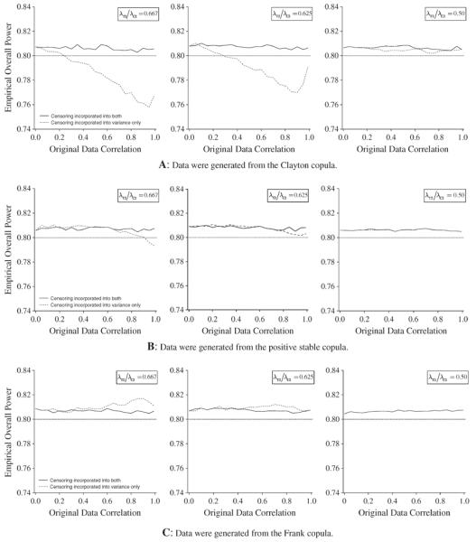
Behavior of the empirical overall power for the log-rank test with common correlation ρ_T = ρ_C = ρ: sample size (equally sized groups: r = 0.5) was calculated to detect the joint reduction in both of the time-to-event outcomes with the overall power of 1 − β = 0.80 at the significance level of α = 0.025, where T₀ = 2 and T = 5, λ_T1/λ_C1 = 0.667 and S_T1(5) = S_T2(5) = 0.5 A: Data were generated from the Clayton copula. B: Data were generated from the positive stable copula. C: Data were generated from the Clayton copula.

These results suggest that the sample sizes calculated by incorporating censoring only into the test statistics variance may be effective for early dependency and symmetric dependence without tail dependency data, even when there is censoring. On the other hand, when the data include late high dependence, censoring should be incorporated into both the test statistics variance and correlation, although it requires extensive computations.

5. SUMMARY AND DISCUSSION

Clinical trials with event-time outcomes as co-primary contrasts are common in many disease areas. In this paper, we outline a simple method for calculating the sample size for randomized superiority trials with two correlated time-to-event outcomes when the time-to-event outcomes are exponentially distributed but censored with different times or censored at the same time. As mentioned in Section 1, the method discussed here can be straightforwardly extended to the issue of competing risks if we can model the competing risks with any bivariate exponential distributions. In addition, this approach provides the foundation for designing randomized trials with other design characteristics including noninferiority clinical trials and trials with more than two primary endpoints. Furthermore, the fundamental results can be used for sizing clinical trials designed to detect an effect on at least one endpoint.

For the co-primary endpoints problem (our primary interest), because the type II error rate increases as the number of outcomes increases, we focused attention on the behavior of power (type II error rate), rather than that of type I error rate. The type I error rate associated with the rejection region H₀ is an increasing function of two values (c₁, c₂) or ($c_1^{\prime }$, $c_2^{\prime }$) given in Section 2. By the analogy of multiple continuous co-primary outcomes as discussed in Hung and Wang [4], the maximum type I error rate is max(Φ(−c₁), Φ(−c₂)) for the two time-to-event outcomes, where Φ(·) is the cumulative function of standard normal distribution. This means that, to investigate whether the type I error rates for testing the joint significance is larger than the nominal level, it is enough to investigate whether the type I error rates for the test for one outcome (marginal) is larger than the nominal level. Then, the behaviors of the type I error rates for the tests for comparing survival curves are well known (e.g., please see Lee, Desu and Gehan [33], Peace and Flora [34], Kellerer and Chmelevsky [35] and so on).

In this paper, to discuss a simpler approach for calculating sample sizes with the two correlated time-to-event outcomes, we assume that the time-to-event outcomes are exponentially distributed. This implies that the method discussed here would work if proportional hazards assumption is satisfied. In real clinical trials, the assumption of constant hazard function may be unrealistic. So that, in actual sample size determinations, one may wish to explore a variety of reasonable scenarios including exponential and nonexponential assumptions. For more general methods, please see Sugimoto et al. [6, 7]. In addition, for other outcomes such as continuous, binary, and their mixed ones, please see Sozu, Sugimoto and Hamasaki [36–38].

REFERENCES

- [1].Gong J, Pinheiro JC, DeMets DL. Estimating significance level and power comparisons for testing multiple endpoints in clinical trials. Controlled Clinical Trials. 2000;21:323–329. doi: 10.1016/s0197-2456(00)00049-0. DOI: 10.1016/S0197-2456(00)00049-0. [DOI] [PubMed] [Google Scholar]
- [2].Offen W, Chuang-Stein C, Dmitrienko A, Littman G, Maca J, Meyerson L, Muirhead R, Stryszak P, Boddy A, Chen K, Copley-Merriman K, Dere W, Givens S, Hall D, Henry D, Jackson JD, Krishen A, Liu T, Ryder S, Sankoh AJ, Wang J, Yeh CH. Multiple co-primary endpoints: medical and statistical solutions. Drug Information Journal. 2007;41:31–46. DOI: 10.1177/009286150704100105. [Google Scholar]
- [3].Chuang-Stein C, Stryszak P, Dmitrienko A, Offen W. Challenge of multiple co-primary endpoints: a new approach. Statistics in Medicine. 2007;26:1181–1192. doi: 10.1002/sim.2604. DOI: 10.1002/sim.2604. [DOI] [PubMed] [Google Scholar]
- [4].Hung HMJ, Wang SJ. Some controversial multiple testing problems in regulatory applications. Journal of Biopharmaceutical Statistics. 2009;19:1–11. doi: 10.1080/10543400802541693. DOI: 10.1080/10543400802541693. [DOI] [PubMed] [Google Scholar]
- [5].Dmitrienko A, Tamhane AC, Bretz F. Multiple Testing Problems in Pharmaceutical Statistics. Chapman & Hall; Boca Raton, FL: 2010. [Google Scholar]
- [6].Sugimoto T, Hamasaki T, Sozu T. Sample size determination in clinical trials with two correlated co-primary time-to-event endpoints. Abstract of the 7th International Conference on Multiple Comparison Procedure; Washington DC, USA. 29 August–1 September 2011. [Google Scholar]
- [7].Sugimoto T, Hamasaki T, Sozu T, Evans S. Sample size determination in clinical trials with two correlated time-to-events endpoints as primary contrasts. The 6th Annual FDA-DIA Statistics Forum; Bethesda, United States. 23–25 April 2012. [Google Scholar]
- [8].Cox DR, Oakes D. Analysis of Survival Data. Chapman & Hall; Boca Raton, FL: 1984. [Google Scholar]
- [9].Kotz S, Johnson NL, Balakrishnan N. Continuous Multivariate Distributions: Models and Applications. John Wiley & Sons; New York: 2000. [Google Scholar]
- [10].Clayton DG. A model for association in bivariate life tables and its application in epidemiological studies of familial tendency in chronic disease. Biometrika. 1976;65:141–151. DOI: 10.1093/biomet/65.1.141. [Google Scholar]
- [11].Hougaard P. Life table methods for heterogeneous populations: distributions describing the heterogeneity. Biometrika. 1984;71:75–83. DOI: 10.1093/biomet/71.1.75. [Google Scholar]
- [12].Hougaard P. A class of multivariate failure time distribution. Biometrika. 1986;73:671–678. DOI: 10.1093/biomet/73.3.671. [Google Scholar]
- [13].Frank MJ. On the simultaneous associativity of F(x, y) and x + y − F(x, y) Aequationes Mathematicae. 1979;19:194–226. DOI: 10.1007/BF02189866. [Google Scholar]
- [14].Genest C. Frank's family of bivariate distribution. Biometrika. 1987;74:549–555. DOI: 10.1093/biomet/74.3.549. [Google Scholar]
- [15].Hsu L, Prentice RL. On assessing the strength of dependency between failure time variables. Biometrika. 1996;83:491–506. DOI: 10.1093/biomet/83.3.491. [Google Scholar]
- [16].Jung SH. Sample size calculation for the weighted rank statistics with paired survival data. Statistics in Medicine. 2009;27:3350–3365. doi: 10.1002/sim.3189. DOI: 10.1002/sim.3189. [DOI] [PubMed] [Google Scholar]
- [17].Prentice RL, Cai J. Covariance and survivor function estimation using censored multivariate failure time data. Biometrika. 1992;73:495–512. DOI: 10.1093/biomet/79.3.495. [Google Scholar]
- [18].Marshall AW, Olkin I. A multivariate exponential distribution. Journal of the American Statistical Association. 1967;62:30–44. DOI: 10.1080/01621459.1967.10482885. [Google Scholar]
- [19].Marshall AW, Olkin I. A generalized bivariate exponential distribution. Journal of Applied Probability. 1967;4:291–302. [Google Scholar]
- [20].Fleischer F, Gaschler-Markefski B, Bluhmki E. A statistical model for the dependence between progression-free survival and overall survival. Statistics in Medicine. 2009;28:2669–2686. doi: 10.1002/sim.3637. DOI: 10.1002/sim.3637. [DOI] [PubMed] [Google Scholar]
- [21].Rosenkranz GK. Another view on the analysis of cardiovascular morbidity/mortality trials. Pharmaceutical Statistics. 2011;10:196–202. doi: 10.1002/pst.434. DOI: 10.1002/pst.434. [DOI] [PubMed] [Google Scholar]
- [22].Machin D, Campbell MJ, Tan SB, Tan SH. Sample Size Tables for Clinical Studies. 3rd Edition John Wiley & Sons; Chichester: 2009. [Google Scholar]
- [23].Collett D. Modelling Survival Data in Medical Research. 2nd Edition Chapman & Hall; Boca Raton, FL: 2003. [Google Scholar]
- [24].Westfall PH, Tobias RD, Rom D, Wolfinger RD, Hochberg Y. Multiple Comparisons and Multiple Tests Using the SAS System. SAS; Cary NC: 1999. [Google Scholar]
- [25].Senn S, Bretz F. Power and sample size when multiple endpoints are considered. Pharmaceutical Statistics. 2007;6:161–170. doi: 10.1002/pst.301. DOI: 10.1002/pst.301. [DOI] [PubMed] [Google Scholar]
- [26].Bretz F, Hothorn T, Westfall P. Multiple Comparisons Using R. Chapman & Hall; Boca Raton, FL: 2011. [Google Scholar]
- [27].Gross AJ, Clark VA. Survival Distributions: Reliability Applications in the Biomedical Science. John Wiley & Sons; New York: 1975. [Google Scholar]
- [28].Lachin E. Introduction to sample size determination and power analysis for clinical trials. Controlled Clinical Trials. 1981;2:93–113. doi: 10.1016/0197-2456(81)90001-5. DOI: 10.1016/0197-2456(81)90001-5. [DOI] [PubMed] [Google Scholar]
- [29].Fleiss JL, Levin B, Paik MC. Statistical Methods for Rates and Proportions. John Wiley & Sons; New York: 2003. [Google Scholar]
- [30].Sugimoto T, Sozu T, Hamasaki T. A convenient formula for calculating sample size of clinical trials with multiple co-primary continuous endpoints. Pharmaceutical Statistics. 2012;11:118–128. doi: 10.1002/pst.505. DOI: 10.1002/pst.505. [DOI] [PubMed] [Google Scholar]
- [31].Fletcher R. Practical Methods of Optimization: Constrained Optimization. Vol. 2. John Wiley & Sons; Chichester: 1981. [Google Scholar]
- [32].Gill PE, Murray W, Wright M. Practical Optimization. Academic Press; London: 1981. [Google Scholar]
- [33].Lee ET, Desu MM, Gehan EA. A Monte Carlo study of the power of same two-sample tests. Biometrika. 1975;62:425–432. DOI: 10.1093/biomet/62.2.425. [Google Scholar]
- [34].Peace KE, Flora RE. Size and power assessments of tests of hypotheses on survival parameters. Journal of the American Statistical Association. 1978;73:129–132. DOI: 10.1080/01621459.1978.10480015. [Google Scholar]
- [35].Kellerer AM, Chmelevsky D. Small-sample properties of censored-data rank tests. Biometrics. 1983;39:675–682. [Google Scholar]
- [36].Sozu T, Sugimoto T, Hamasaki T. Sample size determination in clinical trials with multiple co-primary binary endpoints. Statistics in Medicine. 2010;29:2169–2179. doi: 10.1002/sim.3972. DOI: 10.1002/sim.3972. [DOI] [PubMed] [Google Scholar]
- [37].Sozu T, Sugimoto T, Hamasaki T. Sample size determination in superiority clinical trials with multiple co-primary correlated endpoints. Journal of Biopharmaceutical Statistics. 2011;21:650–668. doi: 10.1080/10543406.2011.551329. DOI: 10.1080/10543406.2011.551329. [DOI] [PubMed] [Google Scholar]
- [38].Sozu T, Sugimoto T, Hamasaki T. Sample size determination in clinical trials with multiple co-primary endpoints including mixed continuous and binary variables. Biometrical Journal. 2012;54:716–729. doi: 10.1002/bimj.201100221. DOI: 10.1002/bimj.201100221. [DOI] [PubMed] [Google Scholar]