Semiparametric Mixed Effect Model with Application to the Longitudinal Knee Osteoarthritis (OAK) Data

Abstract

Motivated by the study of the longitudinal development and progression of knee osteoarthritis (OA) over a 15-year period, this study developed non-parametric mixed-effect models for ordinal outcomes. A stochastic mixed-effect model was used to evaluate the similarity of trajectories associated with increasing disease severity of OA in both knees. Then, a non-parametric mixed-effects model, based on cubic B-splnes, was developed to characterize the unknown nonlinear trend of logits as a function of time1-order. A Markov Transition Model was developed to characterize the transitions among multi-states of knee OA. This newly developed approach allows more flexible functional dependence of the ordinal outcome, levels of increasing knee OA severity, on the covariates.

1. INTRODUCTION AND MOTIVATION

Longitudinal studies, where individuals are measured repeatedly and thus correlated across time, are being developed and applied in diverse fields of research, including epidemiology, health outcomes research, social studies, education and clinical trials, etc. The development and utilization of SAS procedures PROC MIXED and NLMIXED provide increasing flexibility to implement these analyses.

The use of continuous longitudinal outcomes has been well studied, parametrically and non-parametrically [1–6]. However, discrete longitudinal outcomes (binary, counts or categorical nominal or ordinal) may also play an important role in these studies where precise characterization in longitudinal modeling is less developed, e.g. osteoarthritis (OA) evaluated using the 5-level Kellgren and Lawrence (K-L) severity scoring system as described in the Atlas of Standard Radiographs of Arthritis[7]. The OA severity outcome of OA is achieved pictorially and it can be classified into five categories: normal/no disease (state=0), doubtful OA (state=1), minimal OA (state=2), moderate (state=3), and severe (state=4). Further, these five categories represent the initiation and progression of OA and thus is an ordinal variable. Further, as shown in Figure 1, the initiation and progression of knee OA (OAK) can be bidirectional or uni-directional at certain states. This progression is chronic with multiple relapses of symptoms separated by periods with mild or no symptoms [8, 9], and thus can be considered a relapsing-remitting disease [10]. Alternatively, the bi-directionality may reflect the quality of the radiograph that is being scored or the consistency and standardization of those reading the radiographs.

Figure 1.

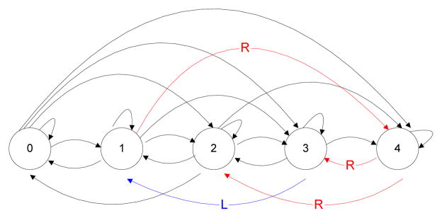
Transition of states of knee OA. Simultaneous transition in both knees (black color);/Right knee only transition (Red color); Left knee only transition (blue color)

The scientific questions of interest in OA studies may include:

• Q1Similarity analysis: whether the knee OA symptoms in both sides develop and progress (longitudinally) at the same/similar pattern?
• Q2Progression analysis: how the knee OA characteristics (probability trajectory of each state) progress over time?
• Q3Transition analysis: how long and under what conditions do the knee OA states transit from one state to other states?

Major approaches can be used to model this type of discrete longitudinal outcomes including marginal models, random-effect models [11–17] and transitional models [10,18–21]. Conceptually, marginal models study the effect of covariates (e.g., age, time, Body Mass Index) on the marginal distribution of the outcome variable and are often called “population-averaged models”. Random-effect models capture individual variability by adding random effects as in regression and are often called “subject-specific models”. Transitional models can be used to evaluate the longitudinal effect of covariates on the state transition patterns of categorical outcome. Computationally, the these models applied to discrete outcomes can implemented using MIXOR[22], BUGS[23], MLwiN[24], HLM6[25], R package DRM [26], or SAS procedures or macros (GENMOD,NLIMIXED, and GLIMMIX, %GLIMMIX) (SAS Institute, Cary, NC).

In the studies and applications, the mean structure of the longitudinal ordinal outcome is frequently assumed to depend on the covariates (e.g., age, time) parametrically. However, the functional forms of covariates may be nonlinear, complex, or even unknown. Thus, the parametric mean assumption may be inappropriate.

Few studies have characterized the longitudinal changes in ordinal OAK trajectories, particularly using parametric or non-parametric functional forms in time (e.g., age). However, there is no evidence that the trajectories of knee OA development and progression over time (e.g., difference score in both knees, probability trajectory of multi-state OA over time) are well modeled by imposing parametric assumptions.

Thus, it is desirable to develop nonparametric approaches to modeling longitudinal ordinal outcomes both in methodology and practice. In this report, we have developed approaches to model the longitudinal ordinal measures using semi-parametric mixed effect modeling, based on cubic B-splines. The methodologies were demonstrated using the longitudinally-acquired knee OA data collected in the Michigan Bone Health and Metabolism Study (MBHMS).

2. BIOLOGICAL, CLINICAL AND EPIDEMIOLOGICAL IMPORTANCE AND RELEVANCE

This approach to modeling longitudinal ordinal outcomes with unknown mean structure is of great importance. Without loss of generality, the methods can be applied to analyze other longitudinal ordinal outcomes apart from knee OA including depression, or functional status. Motivated by the increasing frequency of knee OA of MBHMS over time, this paper develops nonparametric mixed-effects models to study OA development and progression over time.

It is known that osteoarthritis (OA) is a major chronic disease in adults; more than 10 million Americans have knee osteoarthritis (OA), the most commonly studied joint affected by OA. Because of its impact on mobility, knee OA is the most common cause of disability in the United States. Until very recently, knee OA has been considered a disease of the elderly, however, investigations now demonstrate that the development of knee OA is a slowly evolving disease affecting cartilage and bone with notable deterioration in contributing tissues being evident at age 40 with severity increasing over a period of years[8–9, 33–34].

The timing of OA initiation and its progression in the knee and hip is of high interest because these joints, and their integrity, determine the capacity for ambulation. OA accounted for 97% of the total knee replacements and 83% of the total hip replacements in 2004[35]. With national data, the Healthcare Cost and Utilization Project showed osteoarthritis accounted for $10.5 billion in hospital charges in 2006, making this a more expensive condition than pneumonia, stroke, or complications from diabetes. Hospital admissions for arthritis and its treatment more than doubled between 1993 and 2006.

Thus, understanding the development and progression of knee OA, chronologically, is of critical importance for determining when preventive efforts will be most effective and when early diagnosis and treatment of knee OA symptoms should be initiated to slow progression. However, there are few longitudinal studies of knee OA, and there are a dearth of studies that address the development and progression of knee OA. Not only are there few studies that address the initiation and progression of knee OA, the methodologies required to characterize the change in ordinal measures over time is complex, and the most commonly employed measures of OA and its severity from radiographs generate ordinal measures. Further, understanding the relationships of disease initiation and development of OA is made more complex because of the autocorrelation of the contribution by having two knees or two hips contributing to the development of disease.

Due to the complexity in OA data collection, limited data are available with the age range and timing where OAK becomes established. Further, the study of the biological progression mechanisms the time span and natural history of the initiation, progression and transition in knee OA has not been well established. MBHMS provides the opportunity to study this complexity because of its rich longitudinal data bank.

3. METHODS AND MODEL SPECIFICATIONS

In OAK studies, three problems are of interest: similarity of both sides OAK progression; longitudinal progression pattern of OAK severity; and state transition pattern.

3.1 Similarity and Comparison of Left and Right Trajectories Using Difference Score

To compare the development and progression in both knees, the semi-parametric mixed effect model was used [4]:

$$Y_{\mathit{ij}}={\mathbf{X}}_{\mathit{ij}}^T\mathbf{\beta }+f(t_{\mathit{ij}})+{\mathbf{Z}}_{\mathit{ij}}^T{\mathbf{b}}_i+U_i(t_{\mathit{ij}})+{\varepsilon }_{\mathit{ij}}$$ (1)

where: Y_ij is the response variable (e.g., difference score as a continuous variable of right knee and left knee) for the i^th (i = 1,2,…, M, and M is the total number of subjects) subject at time point t_ij (j = 1,2,…, n_i and n_i are the distinct time points for i^th subject); β is a p × 1 vector of regression coefficients associated with covariates X_ij of interest. f (t) is a twice-differentiable smooth function of time; b_i’s are independent q ×1 vectors of random effects associated with covariates Z_ij; U (t_ij) are independent random processes used to model serial correlation; ɛ_ij are independent measurement errors. The fundamental assumptions for this model are: ɛ_ij∼ iid N (0,σ²), b_i ∼ normal (0, D(φ)), D is a positive definite matrix depending on a parameter vector φ; U (t_ij) is a mean zero Gaussian process with covariance function or a non-homogeneous Ornstein-Uhlenbeck (NOU) process, cov(U_i (t), U_j (t))= γ(ζ, α; t, s) depending on a parameter vector ζ and a scalar α, which is used to characterize the variance and correlation of the process U_i (t).

3.2 Semiparametric Mixed Effect Model for Longitudinal Ordinal Data

The ordinal logistic regression models (e.g., proportional odds model, partial-proportional odds model, non-proportional odds model) are widely used for analyzing ordinal outcomes. For repeatedly measured ordinal outcomes across time, mixed–effects models have been developed for ordinal outcome data to account for the dependency inherent in the data[13–15].

For an ordinal response with C categories, the proportional odds model assumes that the effect of an explanatory variable is the same across the C − 1 cumulative logits of the model. This assumption of proportionality across the cumulative odds for all explanatory variables may be too strict and thus a mixed-effect logistic regression model (known as partial-proportional odds): for the cumulative probabilities in terms of the cumulative logits λ_ijc can be formulated as follows

$$\begin{array}{l}{\lambda }_{\mathit{ijc}}=log\left(\frac{P(Y_{\mathit{ij}}\ge c\mid {\mathbf{X}}_{\mathit{ij}},{\mathbf{U}}_{\mathit{ij}},{\mathbf{v}}_i)}{P(Y_{\mathit{ij}}<c\mid {\mathbf{X}}_{\mathit{ij}},{\mathbf{U}}_{\mathit{ij}},{\mathbf{v}}_i)}\right)\hfill \\ ={\gamma }_c+{\mathbf{U}}_{\mathit{ij}}^T{\mathbf{\alpha }}_c+{\mathbf{X}}_{\mathit{ij}}^T\mathbf{\beta }+{\mathbf{Z}}_{\mathit{ij}}^T{\mathbf{v}}_i\hfill \end{array}$$ (2)

where Y_ij is the ordinal response for i^th subject (i = 1,2,…, M, and M is the total number of subjects) measured at j^th time point. c = 1,2,…,C denotes the response categories. X_ij is the p ×1 covariate vector of observation values ij where proportional odds were assumed, and U_ij is the q ×1 vector containing the observation values ij on the set of q covariates where proportional odds were not assumed. Z_ij is the r ×1 vector of random effects for subject i. The Eq. (2) also includes C − 1 strictly decreasing thresholds γ_c. The random effects v_i are assumed to follow a multivariate normal distribution N (0, Σ_v) where Σ_v is the variance-covariance matrix of v_i. The proportionality of a covariate across cumulative odds can be tested using likelihood-ratio test and Akaike’s information criterion (AIC).

Model in Eq. (2) describes the parametric functional form in terms of covariates X_ij and U_ij, e.g., if time variable t (e.g., age) was believed to be cubic polynomial and further assumed non-proportional across cumulative odds, then the “age” term as a fixed effect can be expressed as a function:

$$f(t_{\mathit{ij}})={\beta }_o^c+{\beta }_1^c{t}_{\mathit{ij}}+{\beta }_2^c{t}_{\mathit{ij}}^2+{\beta }_3^c{t}_{\mathit{ij}}^3$$ (3)

In Eq. (3), the coefficients ${\beta }_k^c(k=0,1,2,3)$ depend on category c. In this scenario, without loss of generality, model in Eq. (2) can be rewritten as:

$$\begin{array}{l}{\lambda }_{\mathit{ijc}}=log\left(\frac{P(Y_{\mathit{ij}}\ge c\mid {\mathbf{X}}_{\mathit{ij}},{\mathbf{U}}_{\mathit{ij}},{\mathbf{v}}_i)}{P(Y_{\mathit{ij}}<c\mid {\mathbf{X}}_{\mathit{ij}},{\mathbf{U}}_{\mathit{ij}},{\mathbf{v}}_i)}\right)\hfill \\ ={\gamma }_c+{\mathbf{U}}_{\mathit{ij}}^T{\mathbf{\alpha }}_c+{\mathbf{X}}_{\mathit{ij}}^T\mathbf{\beta }+f(t_{\mathit{ij}})+{\mathbf{Z}}_{\mathit{ij}}^T{\mathbf{v}}_i\hfill \end{array}$$ (4)

However, in most cases, the functional form of f (t_ij) is complex or unknown and Eq. (3) might be not desirable.

Assuming f (t_ij) is twice-differentiable smooth function, and then we can use splines to approximate the form. Splines consist of a series of piecewise polynomials constrained to be joined in a visually smooth fashion and typically formed as an additive combination of locally defined low order polynomials (or basis functions). The proprieties of splines and detailed discussions are widely available [28–32] Cubic B-splines are widely used as a spline basis function and were employed in this study:

$$\stackrel{\sim }{f}(t)=\sum _{k=1}^{q_n}{l}_k{B}_k(t)$$ (5)

where q_n = K_n + 4 and K_n is the total number of internal knots. {B_k,1 ≤ k ≤q_n} are a set of local basis functions (cubic polynomials). Then, f (t) is twice continuously differentiable within the time range.. Assuming non-proportionality of B_k (t_ij) across cumulative odds and replacing f(t_ij) in Eq. (4) by f˜ (t) in Eq. (5), then Eq. (4) becomes:

$$\begin{array}{l}{\lambda }_{\mathit{ijc}}=log\left(\frac{P(Y_{\mathit{ij}}\ge c\mid {\mathbf{X}}_{\mathit{ij}},{\mathbf{U}}_{\mathit{ij}},{\mathbf{v}}_i)}{P(Y_{\mathit{ij}}<c\mid {\mathbf{X}}_{\mathit{ij}},{\mathbf{U}}_{\mathit{ij}},{\mathbf{v}}_i)}\right)\hfill \\ ={\gamma }_c+{\mathbf{U}}_{\mathit{ij}}^T{\mathbf{\alpha }}_c+{\mathbf{X}}_{\mathit{ij}}^T\mathbf{\beta }+\mathbf{B}{(t_{\mathit{ij}})}^T{\mathbf{l}}_c+{\mathbf{Z}}_{\mathit{ij}}^T{\mathbf{v}}_i\hfill \end{array}$$ (6)

After some arithmetic operations, Eq. (6) can be written as:

$$\begin{array}{l}{\lambda }_{\mathit{ijc}}=log\left(\frac{P(Y_{\mathit{ij}}\ge c\mid {\stackrel{\sim }{\mathbf{X}}}_{\mathit{ij}},{\stackrel{\sim }{\mathbf{U}}}_{\mathit{ij}},{\mathbf{v}}_i)}{P(Y_{\mathit{ij}}<c\mid {\stackrel{\sim }{\mathbf{X}}}_{\mathit{ij}},{\stackrel{\sim }{\mathbf{U}}}_{\mathit{ij}},{\mathbf{v}}_i)}\right)\hfill \\ ={\stackrel{\sim }{\gamma }}_c+{\stackrel{\sim }{\mathbf{U}}}_{\mathit{ij}}^T{\mathbf{\alpha }}_c+{\stackrel{\sim }{\mathbf{X}}}_{\mathit{ij}}^T\mathbf{\beta }+{\mathbf{Z}}_{\mathit{ij}}^T{\mathbf{v}}_i\hfill \end{array}$$ (7)

Note that in Eq. (7), parameters α_c’s and β’s have a subject-specific interpretation. Given the covariates X˜_ij, U˜_ij, the probability at category c for the population, π_c (X˜_ij, U˜_ij), can be obtained through:

$$\begin{array}{l}{\pi }_c({\stackrel{\sim }{\mathbf{X}}}_{\mathit{ij}},{\stackrel{\sim }{\mathbf{U}}}_{\mathit{ij}})=E[{\pi }_c^{\mathbf{v}}({\stackrel{\sim }{\mathbf{X}}}_{\mathit{ij}},{\stackrel{\sim }{\mathbf{U}}}_{\mathit{ij}})]\hfill \\ =\underset{\mathbf{v}}{\int }{\pi }_c^{\mathbf{v}}({\stackrel{\sim }{\mathbf{X}}}_{\mathit{ij}},{\stackrel{\sim }{\mathbf{U}}}_{\mathit{ij}})f(\mathbf{v})d\mathbf{v}\hfill \end{array}$$ (8)

For a random intercept model, i.e., ${\mathbf{Z}}_{\mathit{ij}}^T{\mathbf{v}}_i=v_i~N(0,\theta )$, approximately we have:

$${{\lambda }^{\mathit{population}}}_{\mathit{ijc}}\approx {(1+0.346\theta )}^{-1/2}({\gamma }_c+{\stackrel{\sim }{\mathbf{U}}}_{\mathit{ij}}^T{\mathbf{\alpha }}_c+{\stackrel{\sim }{\mathbf{X}}}_{\mathit{ij}}^T\mathbf{\beta })$$ (9)

That is, (1 + 0.346θ)^−1/2 α_c and (1+0.346θ)^−1/2 β has a population-level interpretation that can be expressed in terms of the log odds ratio.

3.3 Transitional Markov Models of Multi-States of Knee OA

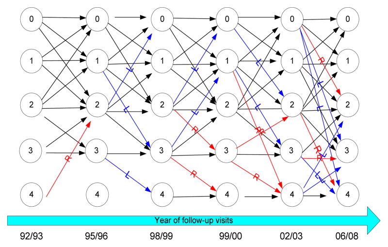
The MBHMS knee OA data showed that the transition patterns between the six adjacent follow-up visits are very complex. The transitions can be stable or bidirectional, i.e., from non-disease to doubtful or any disease, from mild disease to severe disease, or from mild disease to doubtful or even normal states (see Figure 1 and Figure 2).

Figure 2.

MBHMS: multi-state transition of OA in both knees with time on the horizontal axis and severity scores on the vertical axis ranging from zero (no OA) in the tope left hand corner to severe OA in the bottom left hand corner.

Transitional Markov models estimate the transition probabilities between states and examine the effect of covariates on the transition patterns across ordinal responses over time. The q-order mixed effect Markov model can be specified as below:

$$\begin{array}{l}{\lambda }_{\mathit{ijc}}=log\left(\frac{P(Y_{\mathit{ij}}\ge c\mid Y_{\mathit{ij}-1},Y_{\mathit{ij}-2},\cdots ,Y_{\mathit{ij}-q},{\mathbf{X}}_{\mathit{ij}},{\mathbf{U}}_{\mathit{ij}},{\mathbf{v}}_i)}{P(Y_{\mathit{ij}}<c\mid Y_{\mathit{ij}-1},Y_{\mathit{ij}-2},\cdots ,Y_{\mathit{ij}-q},{\mathbf{X}}_{\mathit{ij}},{\mathbf{U}}_{\mathit{ij}},{\mathbf{v}}_i)}\right)\hfill \\ ={\gamma }_c+{\mathbf{U}}_{\mathit{ij}}^T{\mathbf{\alpha }}_c+{\mathbf{X}}_{\mathit{ij}}^T\mathbf{\beta }+\sum _{l=1}^q{\theta }_l{Y}_{\mathit{ij}-l}+{\mathbf{Z}}_{\mathit{ij}}^T{\mathbf{v}}_i\hfill \end{array}$$ (10)

In Eq. (10), the regression coefficients can be interpreted as the effect of covariates on the probability of an ordinal event adjusting for the past history of the process. The estimation procedure and subject-level and population level interpretations of regression coefficients are found in Eq. (7)∼ Eq. (9).

4. APPLICATIONS: LONGITUDINAL KNEE OA

4.1 Data Description

Michigan Bone Health and Metabolism Study (MBHMS) is an on-going population-based longitudinal study of the natural history of reproductive endocrinology. It relates to the initiation and development of musculoskeletal and metabolic diseases and functional limitations in Caucasian women during young and mid-adulthood. It is conducted among women living in and around Tecumseh, Michigan and includes 664 age-eligible (24–44 years in baseline 1992/3) women whose annual assessments cover a 15-year period from 1992/3 through 2006/7, excluding the 18- and 14-month funding lapses in 1997 and 2003, respectively. Radiographs are acquired every three years to assess the status of knee OA initiation and progression. However, women did not have radiographs taken during pregnancy or breastfeeding.

Evaluation of the knee OA data, as part of longitudinal data bank of MBHMS, showed that the initiation and progression over time and the transition patterns are complex. Severity progression can be stable or go both directions, i.e., from non-disease to doubtful or any disease, from mild disease to severe disease, from mild disease to doubtful or even normal states. Figure 2 shows the paths in the K-L severity scores progressing across the six time points when radiographs were available in MBHMS.

As shown in Figure 2, MBHMS knee radiographs were taken in 1992/3, 1995/6, 1998/9, 1999/2000, 2002/3 and 2006/2008. All knee radiographs were taken weight bearing with anterio-posterior positioning. For this particular evaluation, 625 women contributed knee OA scores at one or more time points permitting longitudinal data analyses longitudinal data analyses. Radiographs of the right and left knee were evaluated using the Kellgren and Lawrence (K-L) scoring system described in the Atlas of Standard Radiographs of Arthritis (0=normal/no disease, 1=doubtful OA, 2=minimal OA, 3=moderate OA, and 4=severe OA) pictorially and editorially. This severity score is based on the degree of osteophyte formation, joint space narrowing, sclerosis, and joint deformity. Knee OA was defined as the presence of at least 1 knee with a K-L grade of 2 or higher. There was an extensive quality assurance program in MBHMS to evaluate interrater reproducibility (reliability) as well as standardization in reading films across time to address shifts across time. For the detailed descriptions of osteoarthritis measures, please see references [8–9, 27].

In the analysis, the categories of “moderate OA” and “severe OA” are combined into one category “moderate or severe OA” considering the cell size of “severe OA”, i.e., OA state space is {0 = normal or non-diseased, 1 = doubtful, 2=minimal OA, 3=moderate/severe OA}.

4.2 Results

The mean difference (95% CI) in scores from 28∼60 years old between the right knee and left knee is presented in Figure 3. The data were adjusted for covariates including baseline body mass index (BMI), physical activity, fat mass, skeletal muscle mass and smoking behavior. The significant differences observed between ages 46∼53 indicates that OA in the right knee progressively worsened in comparison to OA of the left knee OA. Two knees were used to define the presence OA in [27]. For illustration purpose, this report used right knee as a representative of OA severity.

Figure 3.

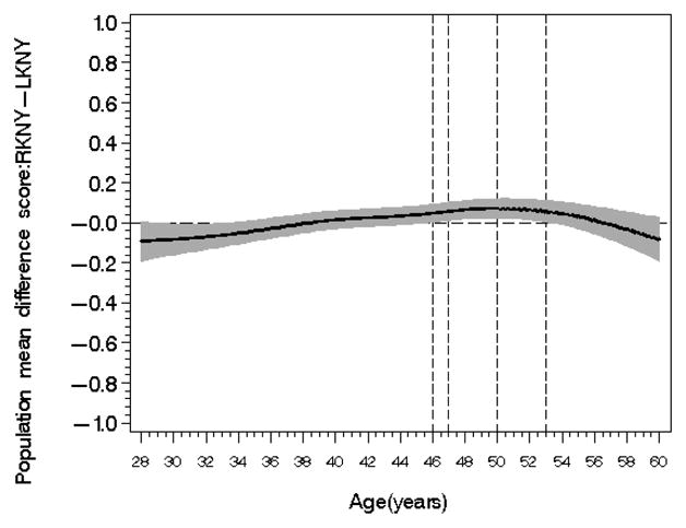
population difference score

In the MBHMS OAK data, there are about 20% of participants (n=121) contributing 3 or less data points from radiographs. Therefore, we used a 1-order (i.e., q = 1) mixed effect Markov model to estimate the probability of observing the transition from an OA state (defined by K-L scores) at a time to the same or different state. Figure 4a–4d showed the selected population transition probability surfaces as a function of age and BMI adjusted for physical activity. The banded gradient surface is the collection transition probabilities given age and BMI. The contour lines connect points on the age and BMI plane that have the same value for transition probability.

Figure 4.

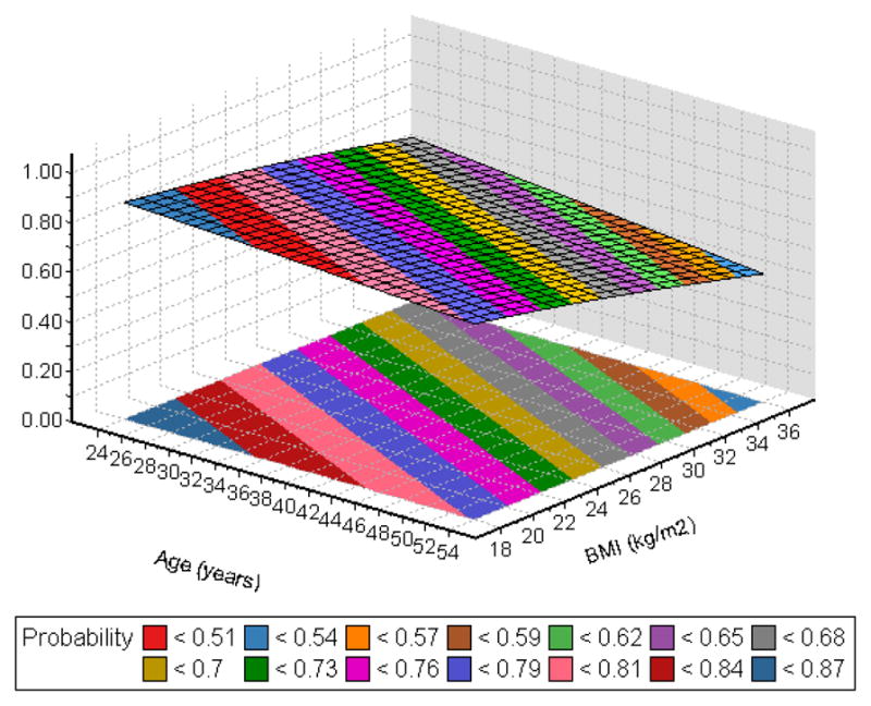
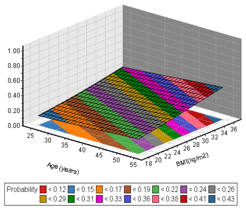
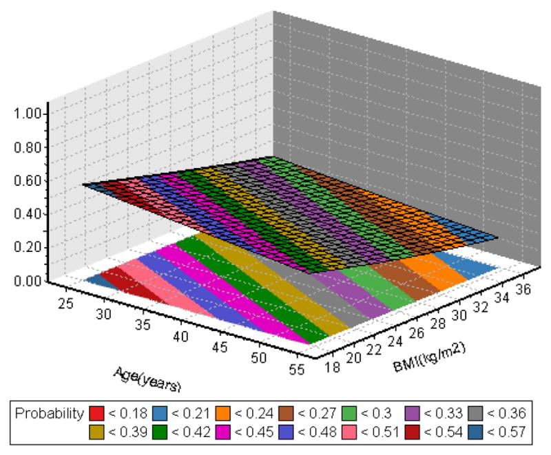
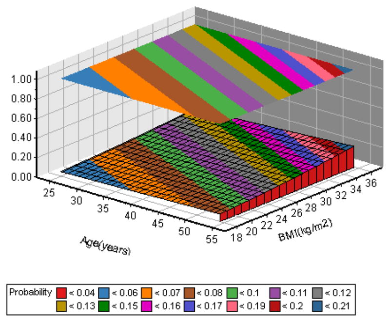
Figure 4a: Transition probability from 0→0

Figure 4b: Transition probability from 0→1

Figure 4c: Transition probability from 1→0

Figure 4d: Transition probability from 1→2

Essentially, this evidence-based study showed that the transition probability from a specific state to a better state (e.g., 1→0, 2→1, 2→0, 3→0, 3→1, 3→2) is monotonically decreasing as women age and/or increase in body size. The probability remaining at the same state (e.g., 0→0,1→1, 2→2, 3→3) or to a worse state (e.g, 0→1, 0→2,0→3, 1→2, 1→3, 2→3) is monotonically increased as women aged and/or increased in body size.

5. CONCLUSIONS AND FUTURE WORK

Motivated by the study of longitudinal development and progression of knee osteoarthritis (OA), this study developed non-parametric mixed-effects models for ordinal outcomes. A stochastic mixed-effect model was used to evaluate the similarity of longitudinal progressive trajectories in both sides of knee OA; A non-parametric mixed-effect model based on cubic B-splne was developed to model the unknown nonlinear trend of logits as a function of time; 1-order Markov Transition model was developed to characterize the transitions among multi-states of knee OA. The developed method allows more flexible functional dependence of the ordinal outcome on the covariates. The future works include: (1) comparison of knots selection stratigies (number and positions, or methods) for cubic B-spline; (2) extension to generalized additive mixed-effects models for more than one covariates with unknow nonlinear functional forms.

References

- 1.Laird NM, Ware JH. Random-Effects Models for Longitudinal Data. Biometrics. 1982;38(4):963–974. [PubMed] [Google Scholar]
- 2.Diggle P, Heagerty P, Liang KY, Zeger S. Analysis of Longitudinal Data. Oxford, U.K.: Oxford University Press; 2002. [Google Scholar]
- 3.Zeger S, Diggle P. Semi-Parametric Models for Longitudinal Data With Applications to CD4 Cell Numbers in HIV Seroconverters. Biometrics. 1994;50(4):689–699. [PubMed] [Google Scholar]
- 4.Zhang D, Lin X, Raz J, Sowers MF. Semiparametric Stochastic Mixed Models for Longitudinal Data. Journal of the American Statistical Association. 1998;93(442):710–719. [Google Scholar]
- 5.Wang JL. Encyclopedia of Biostatistics. 2. John Wiley & Sons, Ltd; 2005. Nonparametric Regression Analysis of Longitudinal Data. [Google Scholar]
- 6.Wand MP, Ormerod JT. On Semiparametric Regression With O’Sullivan Penalized Splines. Australian & New Zealand Journal of Statistics. 2008;50(2):179–198. [Google Scholar]
- 7.Kellgren JH, Lawrence JS. The epidemiology of chronic rheumatism. Philadelphia, PA: F.A. Davis; 1963. Atlas of Standard Radiographs of Arthritis. II. [Google Scholar]
- 8.Sowers MF, Karvonen-Gutierrez CA, Smith RP, Jacobson JA, Jiang Y, Ashton-Miller JA. Knee Osteoarthritis in Obese Women With Cardiometabolic Clustering. Arthritis and Rheumatism. Arthritis Care & Research. 2009;61(10):1328–1336. doi: 10.1002/art.24739. [DOI] [PMC free article] [PubMed] [Google Scholar]
- 9.Sowers MF, Yosef M, Jamadar D, Jacobson JA, Karvonen-Gutierrez CA, Jaffe M. BMI vs. body composition and radiographically-defined osteoarthritis of the knee in women: a 4-year follow-up study. Osteoarthritis Cartilage. 2008;16(3):367–372. doi: 10.1016/j.joca.2007.07.016. [DOI] [PMC free article] [PubMed] [Google Scholar]
- 10.Albert PS. A Markov Model for Sequences of Ordinal Data from A Relapsing-Remitting Disease. Biometrics. 1994;50(1):51–60. [PubMed] [Google Scholar]
- 11.Albert PS. Longitudinal Data Analysis (Repeated Measures) in Clinical Trials. Statistics in Medicine. 1999;18(13):1707–1732. doi: 10.1002/(sici)1097-0258(19990715)18:13<1707::aid-sim138>3.0.co;2-h. [DOI] [PubMed] [Google Scholar]
- 12.Vermunt JK, Hagenaars JA. Methods in Human Growth Research. Cambridge: Cambridge University Press; 2004. Ordinal Longitudinal Data Analysis. [Google Scholar]
- 13.Hedeker D, Demirtas H, Mermelstein RJ. A mixed ordinal location scale model for analysis of Ecological Momentary Assessment (EMA) data. Statistics and its Interface. 2009;2(4):391–401. doi: 10.4310/sii.2009.v2.n4.a1. [DOI] [PMC free article] [PubMed] [Google Scholar]
- 14.Hedeker D, Berbaum M, Mermelstein R. Location-Scale Models for Multilevel Ordinal Data: Between-and Within-Subjects Variance Modeling. Journal of Probability and Statistical Science. 2006;4(1):1–20. [Google Scholar]
- 15.Hedeker D, Gibbons RD. A Random-Effects Ordinal Regression Model for Multilevel Analysis. Biometrics. 1994;50(4):933–944. [PubMed] [Google Scholar]
- 16.Sheu CF. Fitting Mixed-effects Models for Repeated Ordinal Outcomes with the NLMIXED Procedure. Behavior Research Methods, Instruments, & Computers. 2002;34(2):151–157. doi: 10.3758/bf03195436. [DOI] [PubMed] [Google Scholar]
- 17.Colombi R, Forcina A. Marginal regression models for the analysis of positive association of ordinal response variables. Biometrika. 2001;88:1007–1019. [Google Scholar]
- 18.Chen PL, Bernard EJ, Sen PK. A Markov Chain Model Used in Analyzing Disease History Applied to A Stroke Study. Journal of Applied Statistics. 1999;26(4):413–422. [Google Scholar]
- 19.Mandel M, Betensky RA. Estimating Time-Event from Longitudinal Data Using Random-Effects Markov Models: Application to Multiple Sclerosis Progression. Biostatistics. 2008;9(4):750–764. doi: 10.1093/biostatistics/kxn008. [DOI] [PMC free article] [PubMed] [Google Scholar]
- 20.Yang X, Shoptaw S, Nie Kun, Liu J, Belin TR. Markov transition models for binary repeated measures with ignorable and nonignorable missing values. Statistical Methods in Medical Research. 2007;16(4):347–64. doi: 10.1177/0962280206071843. [DOI] [PubMed] [Google Scholar]
- 21.Tutz G. Modelling of Repeated Ordered Measurements by Isotonic Sequential Regression. Statistical Modeling. 2005;5(4):269–287. [Google Scholar]
- 22.Hedeker D, Gibbons RD. MIXOR: A Computer Program for Mixed-Effects Ordinal Regression Aanlysis. Computer Methods and Programs in Biomedicine. 1996;49(2):157–176. doi: 10.1016/0169-2607(96)01720-8. [DOI] [PubMed] [Google Scholar]
- 23.Spiegelhalter DJ, Thomas A, Best NG, Gilks W. BUGS:Bayesian InferenceUsing Gibbs Sampling (Version 0.60) Medical Research Council Biostatistic Unit; Cambridge: 1997. [Google Scholar]
- 24.Yang M, Rashbash J, Goldstein H, Barbosa M. MLwiN Macros for Advanced Multilevel Modeling (V2.0a) Institute of Education, University of London; 2001. [Google Scholar]
- 25.Raudenbusch SW, Bryk AS, Congdon RT. HLM 6 for Windows [Computer software] Lincolnwood, IL: Scientific Software International, Inc.; 2004. [Google Scholar]
- 26.Jokinen J. Doctoral dissertation. University of Helsinki; 2007. Joint Regression and Association Models for Repeated Categorical Responses. [Google Scholar]
- 27.Karvonen-Gutierrez CA, Sowers MF. Sexual Dimorphism in the Association of Cardiometabolic Characteristics and Knee Osteoarthritis Among Obese and Non-Obese Adults: NHANES III, internal report. Department of Epidemiology, the University of Michigan; 2010. [DOI] [PMC free article] [PubMed] [Google Scholar]
- 28.Lu X, Nan B, Song P, Sowers MF. Longitudinal Data Analysis with Event Time as a Covariate. Statistics in BioSciences. 2010;2(1):65–80. [Google Scholar]
- 29.Devlin TF, Weeks BJ. Proc 11th Annual SAS Users Group International. Cary NC: SAS Institute, Inc.; 1986. Spline functions for logistic regression modeling; pp. 646–651. [Google Scholar]
- 30.Stone CJ, Koo CY. Proc Stat Comp Sect Am Statist Assoc. 1985. Additive Splines in Statistics; pp. 45–48. [Google Scholar]
- 31.Wand MP. A Comparison of Regression Spline Smoothing Procedures. Computational Statistics. 2000;15(4):443–462. [Google Scholar]
- 32.Mandel M, Gauthier SA, Guttmann CR, Weiner HL, Betensky RA. Estimating Time to Event From Longitudinal Categorical Data: An Analysis of Multiple Sclerosis Progression. Journal of the American Statistical Association. 2007;102(480):1254–1266. doi: 10.1198/016214507000000059. [DOI] [PMC free article] [PubMed] [Google Scholar]
- 33.Odding E, Valkenburg HA, Algra D, Vandenouweland FA, Grobbee DE, Hofman A. Associations of radiological osteoarthritis of the hip and knee with locomotor disability in the Rotterdam Study. Annals of the Rheumatic Diseases. 1998;57:203–208. doi: 10.1136/ard.57.4.203. [DOI] [PMC free article] [PubMed] [Google Scholar]
- 34.Meulenbelt I, Bijkerk C, Miedema HS, Breedveld FC, Hofman A, Valkenburg HA, Pols HAP, Slagboom PE, van Duijn CM. A genetic association study of the IGF-1 gene and radiological osteoarthritis in a population-based cohort study (the Rotterdam study) Annals of the Rheumatic Diseases. 1998;57:371–374. doi: 10.1136/ard.57.6.371. [DOI] [PMC free article] [PubMed] [Google Scholar]
- 35.The Burden of Musculoskeletal Diseases in the United States. Rosemont, IL: American Academy of Orthopaedic Surgeons; 2008. United States Bone and Joint Decade; pp. 71–96. [Google Scholar]