Exact analytical results for ADC with oscillating diffusion sensitizing gradients

Abstract

The apparent diffusion coefficient (ADC) is analyzed for the case of oscillating diffusion sensitizing gradients. Exact analytical expressions are obtained in the high-frequency expansion of the ADC for an arbitrary number of oscillations N. These expressions are universal and valid for arbitrary system geometry. The validity conditions of the high-frequency expansion of ADC are obtained in the framework of a simple 1D model of restricted diffusion. These conditions are shown to be substantially different for cos- and sin-type gradients: for the cos-type gradients, the high-frequency expansion is valid when the period of a single oscillation is smaller than the characteristic diffusion time, the frequency dependence of ADC being practically the same for any N. In contrast, for the sin-type gradients, the high-frequency regime can be achieved only when the total diffusion time is smaller than the characteristic diffusion time, the frequency dependence of ADC being different for different N.

1. Introduction

Diffusion MRI studies of short-length scales provide a powerful tool for obtaining information on microstructural parameters of porous media and biological systems (e.g., water in the brain, hyperpolarized gases in lung airspaces). It is usually based on measuring the apparent diffusion coefficient (ADC) and calculating the surface-to-volume ratio S/V of restrictions (e.g., [1-3]) by means of the short-time expression [4]

$$D\left(t\right)=D_0\cdot \left[1-c\cdot \frac{1}{d}\cdot \left(\frac{S}{V}\cdot {\left(D_{0}t\right)}^{1∕2}+O\left(D_{0}t\right)\right)\right]$$ (1)

wherein D₀ is the free diffusion coefficient, $c=4∕3\sqrt{\pi }$, d is the system's dimensionality. Importantly, the quantity D(t) in Eq. (1) is not exactly the ADC measured in MRI experiments but a time-dependent (in the general case) effective diffusion coefficient relating the mean square displacement of diffusing particles < (δx)² > and diffusion time t:

$${\langle {\left(\delta x\right)}^2\rangle }_t=2dD\left(t\right)\cdot t.$$ (2)

In the case of free (unrestricted) diffusion, D(t) = D₀, and Eq. (2) reduces to Einstein's relationship < (δx)² >_t = 2dD₀·t. On the other hand, the ADC measured in diffusion MRI experiments, D̃_G(t), is related to the MR signal S(t) by

$${\tilde{D}}_G\left(t\right)=-\frac{1}{b}\cdot \ln \left(\frac{S\left(t\right)}{S_0}\right)$$ (3)

where S₀ is the signal in the absence of diffusion-sensitizing gradients and b is the b-value. The subscript index “G” is used to emphasize that the quantity D̃_G(t) depends, in general, not only on diffusion time t but on a time-course of the diffusion sensitizing gradient as well.

In the case of narrow gradient pulses (NP), the ADC defined by Eq. (3), D̃_NP(t), coincides with D(t) [4] and, therefore, can also be written as in Eq. (1). More generally, the quantities D(t) and D̃_G(t) do not coincide. However, in the Gaussian phase approximation, D̃_G(t) can also be expressed in the form similar to Eq. (1) (e.g., [5-11]):

$${\tilde{D}}_G\left(t\right)=D_0\cdot \left[1-c_G\cdot \frac{S}{dV}{\left(D_{0}t\right)}^{1∕2}\right],$$ (4)

where the coefficient c_G depends on the time-course of diffusion sensitizing gradient. In the case of Hahn echo pulse sequence, the coefficient c_G was obtained in [5]. In [8], a general scheme for calculating the coefficient c_G was applied to the Stejskal-Tanner pulse sequence. The method of calculating the coefficient c_G for the periodic CPMG pulse sequence with an arbitrary number of gradient pairs was proposed in [7] (see also [9, 10, 12]).

It is important to note that Eqs. (1) and (4) are valid under condition that the diffusion time t is much smaller than the characteristic diffusion time t_D,

$$t\ll t_D=\frac{1}{D_0{(S∕dV)}^2}$$ (5)

On the other hand, reliable MR measurements require a sufficient dynamic range of the MR signal, i.e., sufficiently high b-values. Achieving high b in the short-time regime is a technically challenging problem. A promising way to get into the short-time limit is to apply high-frequency oscillating gradients (OG) [13-15], which are now intensively used for studying short-length scales (e.g., [11, 16-18]). For OG experiments, diffusion time t in Eq. (4) can be effectively substituted (at least, in some cases, see below) by the period of a single oscillation T which can be chosen to be short enough to satisfy the inequality $T\ll t_D$. At the same time, the b value is proportional to a number of oscillations N and, therefore, can be made high enough to achieve a sufficient dynamic range of the MR signal.

Despite rather intensive use of OG in recent MR studies, analytical expressions for the coefficient c_G in Eq. (4), corresponding to the OG with a finite number of oscillations N, have not been reported yet. Numerically, the coefficient c_G for cos- and sin-type gradients was considered in [11]; an analytical expression for this coefficient was found only in the limiting case N → ∞ [19].

In the present paper, we derive exact analytical expressions for the coefficient c_G for an arbitrary number of oscillations (Section 2). Besides, we will consider the time dependence of ADC beyond the short-time regime in a simple one-dimensional (1D) model (Section 3) and find the interval of validity of the short-time (high-frequency) expansion of ADC. As we will see, there is a considerable difference between the OG of cos- and sin- types. The calculations are based on the Gaussian phase approximation and widely accepted understanding that the ensemble-averaged phase accumulated by diffusing particles is equal to 0 (the last assumption is under discussion for confined diffusion in [20]). The validity of the results is confirmed by numerical solution of Bloch-Torrey equations in the framework of the multi-propagator approach [21, 22] and by Monte-Carlo simulations.

2. Short diffusion time. Arbitrary geometry

First, we remind a general scheme for calculating the coefficient c_G for an arbitrary waveform for diffusion sensitizing gradients (e.g., [5, 6]).

In the Gaussian phase approximation (valid at sufficiently low b values), the time-dependent ADC, D̃_G(t), can be expressed in terms of the mean square displacement and, consequently, according to Eq. (2), via D(t):

$$b{\tilde{D}}_G\left(t\right)=-\frac{{\gamma }^2}{2}{\int }_0^{t}d{\tau }_1{\int }_0^{{\tau }_1}d{\tau }_{2}g\left({\tau }_1\right)g\left({\tau }_2\right)\cdot {\langle {\left(\delta x\right)}^2\rangle }_{({\tau }_1-{\tau }_2)}=-{\gamma }^2{\int }_0^{t}d{\tau }_1{\int }_0^{{\tau }_1}d{\tau }_{2}g\left({\tau }_1\right)g\left({\tau }_2\right)\cdot ({\tau }_1-{\tau }_2)\cdot D({\tau }_1-{\tau }_2)$$ (6)

where γ is the gyromagnetic ratio, g(τ) is the time–dependent diffusion sensitizing field gradient (the condition $G\left(t\right)={\int }_0^{t}d\tau g\left(\tau \right)=0$ and a homogeneous initial spin distribution are assumed; note that if at least one of these assumptions is not fulfilled, Eq. (6) should be modified to take into account the mean value of phase accumulated by diffusing particles [14]). Substituting Eq. (1) into Eq. (6), the quantity D̃_G(t) can be rewritten as

$${\tilde{D}}_G\left(t\right)=-\frac{{\gamma }^2}{b}{D}_0\cdot {\int }_0^{t}d{\tau }_1{\int }_0^{{\tau }_1}d{\tau }_{2}g\left({\tau }_1\right)g\left({\tau }_2\right)\cdot ({\tau }_1-{\tau }_2)\cdot \left\{1-c\cdot \frac{S}{dV}\cdot {[D_0\cdot ({\tau }_1-{\tau }_2)]}^{1∕2}\right\}.$$ (7)

It is easy to verify that the first term in the expression is identically equal to the standard representation of the b value,

$$-{\gamma }^2\cdot {\int }_0^{t}d{\tau }_1{\int }_0^{{\tau }_1}d{\tau }_{2}g\left({\tau }_1\right)g\left({\tau }_2\right)\cdot ({\tau }_1-{\tau }_2)={\gamma }^2\cdot {\int }_0^{t}d\tau \left[{\int }_0^{\tau }\right]d{\tau }_{1}g{\left({\tau }_1\right)}^2=b.$$ (8)

The coefficient c_G appearing in Eq. (4) can then be expressed as

$$c_G=c\cdot \frac{I_{3∕2}^{\left(G\right)}\left(t\right)}{I_1^{\left(G\right)}\left(t\right)},$$ (9)

where

$$I_n^{\left(G\right)}\left(t\right)={\int }_0^{t}d{\tau }_1{\int }_0^{{\tau }_1}d{\tau }_{2}g\left({\tau }_1\right)g\left({\tau }_2\right)\cdot {({\tau }_1-{\tau }_2)}^n$$ (10)

(notations are slightly modified from those in [6]). Equation (10) makes it possible to calculate the coefficient c_G for an arbitrary gradient time-course g(τ).

Let us consider the diffusion sensitizing oscillating gradient of the form:

$$g\left(\tau \right)=g_0\cdot \cos (\omega \tau -\phi )$$ (11)

where g₀ is an amplitude, ω is the frequency of oscillations, and φ is an arbitrary phase. The particular cases of the cos- and sin-type gradients correspond to φ = 0 and φ = π/2, respectively. The total diffusion sensitizing gradient waveform consists of N full periods of oscillations, applied for duration t = N·T = N·2π/ω. The gradient waveform is preceded by the 90° RF pulse and the signal is acquired at τ > t = NT (actually, the signal can be acquired at intermediate time points τ_m = mT, m = 1,2,...,N at which the condition G(t_m) = 0 is fulfilled).

The b value corresponding to the gradient waveform (11), b_N, is a sum of b values corresponding to a single oscillation, b₁:

$$b_N=N\cdot b_1,b_1={\left(\gamma g_0\right)}^2\cdot \frac{\pi }{{\omega }^3}\cdot \left(1+2{\sin }^2\phi \right)$$ (12)

It is convenient to rewrite the expansion of ADC, Eq. (4), in terms of oscillation frequency ω and a number of oscillations N:

$${\tilde{D}}_G(t=2\pi N∕\omega )=D_0\cdot \left[1-c_G\cdot \frac{S}{dV}{\left(D_0\cdot \frac{2\pi N}{\omega }\right)}^{1∕2}\right]==D_0\cdot \left(1-\frac{c_G^{\prime }}{{\Omega }^{1∕2}}\right),c_G^{\prime }=c_G\cdot {\left(2\pi N\right)}^{1∕2}$$ (13)

where the dimensionless frequency Ω = ωt_D is introduced.

The coefficient c′ (hereafter we will omit the subscript G) depends on N and the phase φ, c′ = c′(φ, N). It can be found by means of direct evaluation of the double-integrals (10):

$$c^{\prime }(\phi ,N)=\frac{32\pi N^{3∕2}{\sin }^2\phi +12\pi N\cdot \mathrm{C}\left(2N^{1∕2}\right)+3(3+4{\sin }^2\phi )\cdot \mathrm{S}\left(2N^{1∕2}\right)}{6\sqrt{2}\pi N(1+2{\sin }^2\phi )}$$ (14)

where C(x) and S(x) are the Fresnel functions.

In the particular case of the cos-type gradient (φ = 0),

$$c_{\cos }^{\prime }\left(N\right)\equiv c^{\prime }(0,N)=\frac{4\pi N\cdot \mathrm{C}\left(2N^{1∕2}\right)+3\cdot \mathrm{S}\left(2N^{1∕2}\right)}{2\sqrt{2}\pi N}$$ (15)

For the sin-type gradient (φ = π/2),

$$c_{\sin }^{\prime }\left(N\right)\equiv c^{\prime }(\pi ∕2,N)=\frac{32\pi N^{3∕2}+12\pi N\cdot \mathrm{C}\left(2N^{1∕2}\right)+21\cdot \mathrm{S}\left(2N^{1∕2}\right)}{18\sqrt{2}\pi N}$$ (16)

The dependence of the coefficient c′ on the number of oscillations N is shown in Fig. 1 for different values of φ (shown by the lines).

Figure 1.

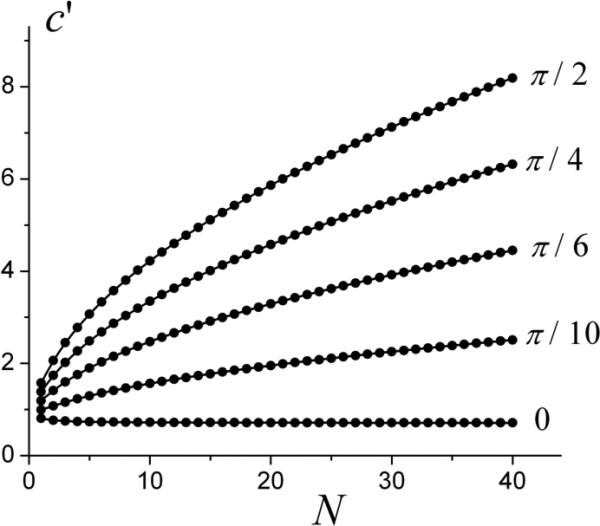
The dependence of the coefficient c′(φ, N) on oscillation number N for different phase φ (shown by numbers by the line).

Importantly, for any φ ≠ 0 (including sin-type gradient), the coefficient c′(φ, N) monotonically increases at large N (as $\sqrt{N}$), whereas for φ = 0 (cos-type gradient), the coefficient c′(0, N) monotonically decreases with N increases and tends to a finite value:

$$\begin{array}{cc}\hfill & c_{\cos }^{\prime }\left(N\right)\equiv c^{\prime }(\phi =0,N)=\frac{1}{\sqrt{2}}\cdot \left(1-\frac{1}{{\pi }^2{N}^{3∕2}}\right),N>>1\hfill \\ \hfill & c^{\prime }(\phi \ne 0,N)=\frac{8\sqrt{2}{\sin }^2\phi }{3(1+2{\sin }^2\phi )}\cdot N^{1∕2},N>>1\hfill \end{array}$$ (17)

The limiting value of $c_{\text{cos}}^{\prime }(N\to \infty )=1∕\sqrt{2}$ exactly coincides with the result obtained in [19] in the framework of the frequency domain approach. Note also the coefficient $c_{\text{cos}}^{\prime }\left(N\right)$ tends to its limiting value rather fast and varies in a rather narrow interval (from 0.81 for N = 1 to 0.71 at N → ∞; the relative difference between $c_{\text{cos}}^{\prime }(N>5)$ and $c_{\text{cos}}^{\prime }(N\to \infty )$ does not exceed 3%).

The divergence of the coefficient c′(φ ≠ 0, N) at large N imposes a restriction on the oscillation number N because the expansion (13) is valid only under condition $c^{\prime }(\phi \ne 0,N)∕{\Omega }^{1∕2}\ll 1$. Using the second line in Eq. (17), this condition can be re-written as $\Omega \gg N\cdot {\text{sin}}^4\phi$, or $t\ll t_D∕{\text{sin}}^4\phi$. Thus, for any φ not too close to 0 (including the sin-type gradient), the total duration of the diffusion-sensitizing waveform must be smaller than the characteristic time t_D.

Although there is no such a restriction for the cos-type gradient ($c_{\text{cos}}^{\prime }\sim 1$ for any N), and the expansion (13) is formally valid under condition $\Omega \gg 1$, we should remind that all the expressions in Eqs. (14)-(17) are derived based on Eq. (1) which is valid only at short total diffusion time $t:t\ll t_D$, Eq. (5). In the next section, however, we demonstrate that expressions similar to Eq. (13) can be obtained without using the short-time expansion of D(t), Eq. (1). For this purpose, we will explore a simple 1D model of restricted geometry, for which an exact solution to the diffusion problem (diffusion propagator, means square displacement, etc.) are available for arbitrary time t.

3. Arbitrary diffusion time. 1D geometry

Consider particles diffusing within the segment x = [0, a] and restricted by impermeable boundaries. The propagator for this model, determining the probability for diffusion from x₀ to x during time t, is well known (e.g., [23]):

$$P(x,x_0,t)=\frac{1}{a}\cdot \left[1+2\cdot \sum _{n=-\infty }^{+\infty }\cos \frac{\pi nx}{a}\cos \frac{\pi n{x}_0}{a}\exp (-{\lambda }_{n}t)\right]$$ (18)

where the eigenvalues λ_n = D₀(πn / a)². Using Eq. (18), the mean square displacement < (δx)² > and , correspondingly, the time-dependent diffusion coefficient D(t), Eq. (2), can be readily calculated:

$$D\left(t\right)=\frac{1}{2at}\cdot {\int }_0^a{\int }_0^{a}dxd{x}_0{(x-x_0)}^{2}P(x,x_0,t)==\frac{a}{12t}\cdot \left[1-\frac{96}{{\pi }^4}\cdot \sum _{n=2k-1}^{\infty }\frac{\exp (-{\lambda }_{n}t)}{n^4}\right]$$ (19)

It can be verified that the short-time behavior of D(t), at $t\ll t_D=a^2∕4D_0$, is given by Eq. (1) with S / V = 2 / a. Note that for this purpose, it is convenient to use another well-known representation of the propagator (e.g., [23]),

$$P(x,x_0,t)=\frac{1}{{\left(4\pi D_{0}t\right)}^{1∕2}}\cdot \sum _{n=-\infty }^{+\infty }\left[\exp \left(-\frac{{(x-x_0+2na)}^2}{4D_{0}t}\right)+\exp \left(-\frac{{(x+x_0+2na)}^2}{4D_{0}t}\right)\right]$$ (20)

In what follows, we consider the cos-type and sin-type oscillating gradients separately. Substituting Eq. (19) into Eq. (6) and using Eq. (12) for the b value, we get

$${\tilde{D}}_{\cos }=D_0\cdot \frac{128{\Omega }^2}{{\pi }^{2}N}\cdot \sum _{n=2k-1}^{\infty }\frac{[N\cdot ({\pi }^4{n}^4+16{\Omega }^2)-4\pi n^2\Omega \cdot (1-\exp (-{\pi }^{3}N{n}^2∕2\Omega ))]}{n^2{({\pi }^4{n}^4+16{\Omega }^2)}^2}$$ (21)

$${\tilde{D}}_{\sin }=D_0\cdot \frac{128{\Omega }^2}{3{\pi }^{5}N}\cdot \sum _{n=2k-1}^{\infty }\frac{[{\pi }^{3}N{n}^2\cdot ({\pi }^4{n}^4+16{\Omega }^2)+64{\Omega }^3\cdot (1-\exp (-{\pi }^{3}N{n}^2∕2\Omega ))]}{n^4{({\pi }^4{n}^4+16{\Omega }^2)}^2}$$ (22)

The dependence of D̃_cos on the dimensionless frequency Ω at different N (calculated numerically from Eq. (21)) is shown in Fig. 2a. Importantly, the quantity D̃_cos depends only on Ω and is practically independent of the number of oscillations for N > 5. This property of the quantity D̃_cos can be readily understood by noticing that the second term in the numerator in Eq. (21) is small as compared to the first one. Neglecting this small term, the sum in Eq. (21) can be obtained in a closed analytical form:

$${\tilde{D}}_{\cos }=D_0\cdot F\left(\Omega \right),F\left(\Omega \right)=1-\frac{1}{{\left(2\Omega \right)}^{1∕2}}\cdot \frac{\sinh \left({\left(2\Omega \right)}^{1∕2}\right)+\sin \left({\left(2\Omega \right)}^{1∕2}\right)}{\cosh \left({\left(2\Omega \right)}^{1∕2}\right)+\cos \left({\left(2\Omega \right)}^{1∕2}\right)}$$ (23)

As expected, the number of oscillations N does not enter Eq. (23).

Figure 2.

The frequency dependence of ADCs D̃_cos (a) and D̃_sin (b) for different number oscillation N.

The asymptotic behavior of the function F(Ω) at low and high frequency is:

$$F\left(\Omega \right)=\{\begin{array}{c}\frac{2}{15}{\Omega }^2,\Omega \ll 1\hfill \\ 1-\frac{1}{{\left(2\Omega \right)}^{1∕2}},\Omega \gg 1\hfill \end{array}\phantom{\}}$$ (24)

Hence, the high-frequency behavior of D̃_cos in Eqs. (23)-(24) exactly coincides with the result of the previous section, Eq. (13), with the limiting value of $c^{\prime }=1∕\sqrt{2}$. Importantly, Eq. (23) is derived without the assumption $t=NT\ll t_D$ (as assumed when deriving Eq. (13)). This means that the high-frequency asymptotic behavior of D̃_cos is valid under the much softer condition $\Omega \gg 1$, or $T\ll t_D$ : the period of a single oscillation T (rather than the total duration t of the oscillating-gradient waveform) should be small as compared to the characteristic time t_D.

The situation with the sin-type gradient is substantially different: the quantity D̃_sin strongly depends not only on Ω but on the number of oscillations N, as illustrated in Fig. 2b. It is easy to verify from Eq. (22) that in the interval $1\ll \Omega \ll N$, ${\tilde{D}}_{\text{sin}}\approx \frac{1}{3}{D}_0$, as demonstrated in Fig. 3b by the line corresponding to N = 100. And only in the case $\Omega \gg N$, the quantity D̃_sin is described by the expression as in Eq. (13):

$${\tilde{D}}_{\sin }(\Omega ,N)=D_0\cdot \left[1-\frac{c_{\sin }^{\prime }\left(N\right)}{{\Omega }^{1∕2}}\right],\Omega >>N$$ (25)

where the coefficient $c_{\text{sin}}^{\prime }\left(N\right)$ is given by Eq. (16).

Figure 3.

Comparison of the ADCs D̃_cos (a) and D̃_sin (b-d) (solid lines) with the high-frequency approximation (dashed lines), Eq. 13, for different number oscillation N. As the quantity D̃_cos is practically independent of N, only one line (corresponding to N = 20) is shown in Fig. 3a.

In Figure 3 the dependences of D̃_cos (a) and D̃_sin (b, c, d) on Ω for different N, calculated from Eq. (21)-(22) (solid lines), are shown. The dashed lines illustrate the high-frequency asymptotic described by Eqs. (23)-(25) (with the corresponding values of the coefficient c′). The vertical dotted lines show the approximate thresholds after which two lines are practically indistinguishable and the high-frequency approximation can be used.

As we see in Fig. 3a, the exact frequency dependence D̃_cos and its high-frequency asymptotic practically coincide at Ω > 5. Importantly, this result is valid for any total number of oscillation N, meaning that the high-frequency asymptotic behavior of D̃_cos takes place under condition T < t_D / 5 regardless of N. In contrast, the range of validity of the high-frequency behavior of D̃_sin, Eq. (25), strongly depends on N and is achieved when (roughly) Ω > 5N, as demonstrated in Fig. 3b-d. Thus, the high-frequency approximation of D̃_sin takes place under condition t = NT < t_D / 5, i.e. when the total diffusion time t is small enough as compared to the characteristic diffusion time t_D.

Although the results of this section are obtained for the 1D diffusion model, they can be readily generalized for an arbitrary model with known eigenfunction representation of the diffusion propagator P(r, r₀, t), e.g., for diffusion within a cylinder or sphere.

Discussion

Diffusion sensitizing oscillating gradients are usually used to probe diffusion in the short-time regime, Eq.(1), in which diffusion time t is effectively substituted by oscillation period T = 2π / ω, Eq. (13) (e.g., for obtaining information on the surface-to-volume ratio). Although T can be chosen short enough (the high-frequency range), the b value, accumulated over many periods of oscillations, leads to a sufficient signal dynamic range (as b ∝ N, Eq. (12)). Obviously, this main idea of utilizing the oscillation gradients “works” under condition that D̃ can be described by Eq. (13). As shown above, this approach holds for the cos-type gradient but fails for the sin-type gradient. For the latter, the short-time (high-frequency) expansion, Eq. (13), is valid only when the total duration of the diffusion-sensitizing gradient waveform, t, is smaller than the characteristic diffusion time t_D. Consequently, although the sin-type gradient leads to a 3-times higher b value than the cos-type gradient (given ω and N, see Eq. (12)), its application to short-time experiments becomes rather questionable.

MR signals obtained with oscillating gradients are usually analyzed in the frequency domain (e.g., [13, 14, 17, 19, 24]). However, such an approach becomes problematic when analyzing the sin-type gradient (more generally, oscillating gradients with arbitrary phase φ in Eq. (11)). The problem is related to the presence of the δ-function peculiarity at ν = 0 in the gradient modulation spectrum, F_G(ν),

$$F_G\left(\nu \right)=\gamma \cdot {\int }_{-\infty }^{+\infty }d{t}_1\exp \left(i\nu t_1\right){\int }_0^{t_1}d{t}_{2}g\left(t_2\right)$$ (26)

For the gradients in Eq. (11), this spectrum is a combination of the δ-functions [13-15, 17]:

$$F(\nu ,\omega ;\phi )=\frac{\pi \gamma g_0}{\omega }\cdot \{[\delta (\nu -\omega )+\delta (\nu +\omega )]\cdot i\exp (-i\phi )+2\delta \left(\nu \right)\cdot \sin \phi \}$$ (27)

The MR signal as a function of frequency ω is given by

$$S=S_0\cdot \exp \left[-\frac{1}{\pi }\cdot {\int }_0^{\infty }d\nu F(-\nu ,\omega )U\left(\nu \right)F(\nu ,\omega )\right]$$ (28)

where U(ν) is the Fourier transform of the velocity autocorrelation function. The gradient modulation spectrum, Eq. (27), “cut out” the ω-component and zero-frequency component from the correlation function U. The substantial difference between so called “ac” pulse sequences (sequences without the zero-frequency component) and “dc” pulse sequences (with zero-component) was demonstrated in [14, 15] by the example of CPMG pulse sequences with different positions of RF pulses with respect to gradient pulses.

The cos-type gradient is an analog of the CPMG pulse sequence with 180° RF pulses “correctly” positioned at T / 4, 3T / 4, ... that leads to the “ideal” frequency sampling function with a single “cut-out” component (effectively, the CPMG pulse sequence is a box-type oscillating gradient obtained by applying a constant gradient and a series of 180° RF pulses, Fig. 4a). As demonstrated in [19], the limiting value $c_{\text{cos}}^{\prime }(N\to \infty )=1∕\sqrt{2}$ is very close to that obtained for the CPMG pulse sequence: $c_{CPMG}^{\prime }=c_{\text{cos}}^{\prime }\cdot 0.9935$ at N → ∞. Our calculations revealed a rather similar behavior of the coefficients $c_{CPMG}^{\prime }$ and $c_{\text{cos}}^{\prime }$ for arbitrary N. The dependence of the coefficients $c_{\text{cos}}^{\prime }\left(N\right)$ and $c_{CPMG}^{\prime }\left(N\right)$ on N is illustrated in Fig.4 (the coefficient $c_{CPMG}^{\prime }\left(N\right)$ is re-calculated from the function C(N) given in Table in [12]: $c_{CPMG}^{\prime }\left(N\right)=-C\left(N\right)∕2N\cdot {(\pi ∕2)}^{1∕2}$; details of elegant calculations of C(N) for the CPMG sequence can be found in [7]). For large sufficiently N (N > 20), both the coefficients are very similar and can be described by the first line of Eq. (17).

Figure 4.

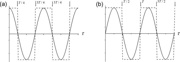
(a) The cos-type gradient (solid line) and the effective CPMG pulse sequence of the same gradient amplitude (dashed line); the 180° RF pulses in the CPMG (shown by arrows) “correctly” positioned at T / 4, 3T / 4, .... (b) the sin-type gradient (solid line) and the effective “shifted” CPMG-like pulse sequence (dashed line); the 180° RF pulses positioned at T / 2, T, ....

As demonstrated in [14, 15], slightly different positioning of the RF pulses leads to “a dramatic change”, namely, to the appearance of a dominant zero-frequency component which hinders the sampling of the spectral density. In our case, such a “different positioning” is an analog of the non-zero phase φ (180° RF pulses positioned at T / 2, T, 3T / 2, ... correspond to φ = π / 2, i.e., to the sin-type gradient, Fig. 4b).

For sufficiently high frequency, the ω-component of the function U in Eq. (28), can be found as the Fourier transform of the short-time expansion of the diffusion coefficient D(t), Eq. (1) [19]. As properly mentioned in [19], the expansion (1) has finite or even zero radius of convergence and, consequently, its frequency counterpart should be used only within certain boundaries. However, the latter have not been established. Importantly, the dc component, i.e. U(ν → 0), requires knowledge of D(t) in the long-time regime (note that for any restricted geometry, D(t) → 0 at t → ∞). That is why the frequency-domain approach based on Eqs. (26)-(28) cannot provide an adequate expression for ADC for the gradients with φ ≠ 0 (including the sin-type gradient as a particular case).

Our approach based on calculations in the time domain lacks such problems. More importantly, it allows calculations of ADC not only in the limiting case N → ∞ but for arbitrary number of oscillation N.

Conclusion

In the present paper we analyze the ADC corresponding to the oscillating diffusion sensitizing gradients. First, starting from the short-time expansion of the diffusion coefficient D(t), Eq.(1), the exact analytical expressions for the coefficient c′ in the high-frequency expansion of the ADC, Eq. (13), were found for an arbitrary number of oscillations N. These expressions are universal and valid for arbitrary system geometry. Secondly, in the framework of the simple 1D model of restricted diffusion, the ADC was analyzed for an arbitrary frequency ω and oscillation number N. It was shown that the validity condition of the high-frequency expansion of the ADC is substantially different for the cos- and sin-type gradients. For the cos-type gradients, this high-frequency regime is reached when the period of a single oscillation is smaller than the characteristic diffusion time t_D, the coefficient $c_{\text{cos}}^{\prime }\left(N\right)$ monotonically decreasing to its limiting value. Besides, the frequency dependence of the ADC is practically the same for any N > 5. In contrast, for the sin-type gradient, the high-frequency regime can be achieved only when the total duration of the oscillating gradient waveform is smaller than t_D, the coefficient $c_{\text{sin}}^{\prime }\left(N\right)$ monotonically increasing with N and the frequency dependence of the ADC being different for different N. These results should be taken into consideration for correct interpretation of experimental data in MR experiments utilizing oscillating gradients.

Highlights.

• Apparent diffusion coefficient is analyzed for the case of oscillating diffusion gradients.

• Exact analytical expressions are found in the high-frequency expansion of ADC.

• For the 1D model, the validity conditions of the high-frequency expansion of ADC are obtained.

• These conditions are shown to be substantially different for cos- and sin-type gradients.

Figure 5.

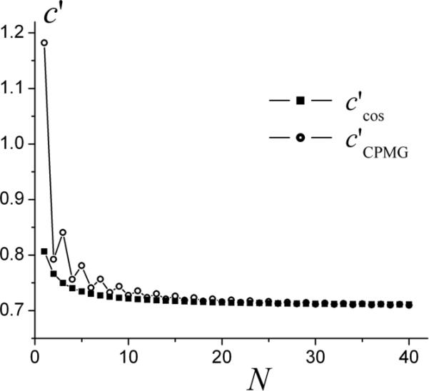
The comparison of the coefficients c′ for the cos-type oscillating gradient (squares) and CPMG pulse sequence (circles).

References

- 1.Latour LL, Mitra PP, Kleinberg RL, Sotak CH. Time-dependent diffusion coefficient of fluids in porous media as a probe of surface-to-volume ratio. J. Magn. Reson. Ser. A. 1993;101:342–346. [Google Scholar]
- 2.Latour LL, Svoboda K, Mitra PP, Sotak CH. Time-dependent diffusion of water in a biological model system. Proc Natl Acad Sci U S A. 1994;91:1229–1233. doi: 10.1073/pnas.91.4.1229. [DOI] [PMC free article] [PubMed] [Google Scholar]
- 3.Mair RW, Wong GP, Hoffmann MD, et al. Probing porous media with gas diffusion NMR. Phys. Rev. Lett. 1999;83:3324. doi: 10.1103/PhysRevLett.83.3324. [DOI] [PubMed] [Google Scholar]
- 4.Mitra PP, Sen PN, Schwartz LM. Short-time behavior of the diffusion coefficient as a geometrical probe of porous media. Phys Rev B Condens Matter. 1993;47:8565–8574. doi: 10.1103/physrevb.47.8565. [DOI] [PubMed] [Google Scholar]
- 5.de Swiet TM, Sen PN. Decay of nuclear magnetization by bounded diffusion in a constant field gradient. J. Chem. Phys. 1994;100:5597–5604. [Google Scholar]
- 6.Fordham EJ, Mitra PP, Latour LL. Effective diffusion times in multiple-pulse PFG diffusion measurements in porous media. J Magn Reson., Ser. A. 1996;121:187–192. [Google Scholar]
- 7.Axelrod S, Sen PN. Nuclear magnetic resonance spin echoes for restricted diffusion in an inhomogeneous field: Methods and asymptotic regimes. J. Chem. Phys. 2001;114:6878–6895. [Google Scholar]
- 8.Zielinski LJ, Sen PN. Effects of finite-width pulses in the pulsed-field gradient measurement of the diffusion coefficient in connected porous media. J Magn Reson. 2003;165:153–161. doi: 10.1016/s1090-7807(03)00248-9. [DOI] [PubMed] [Google Scholar]
- 9.Zielinski LJ, Hurlimann MD. Probing short length scales with restricted diffusion in a static gradient using the CPMG sequence. J Magn Reson. 2005;172:161–167. doi: 10.1016/j.jmr.2004.10.006. [DOI] [PubMed] [Google Scholar]
- 10.Stepisnik J, Lasic S, Mohoric A, Sersa I, Sepe A. Spectral characterization of diffusion in porous media by the modulated gradient spin echo with CPMG sequence. J Magn Reson. 2006;182:195–199. doi: 10.1016/j.jmr.2006.06.023. [DOI] [PubMed] [Google Scholar]
- 11.Parsons EC, Jr., Does MD, Gore JC. Temporal diffusion spectroscopy: theory and implementation in restricted systems using oscillating gradients. Magn Reson Med. 2006;55:75–84. doi: 10.1002/mrm.20732. [DOI] [PubMed] [Google Scholar]
- 12.Sen PN, Andre A, Axelrod S. Spin echoes of nuclear magnetization diffusing in a constant magnetic field gradient and in a restricted geometry. J Chem Phys. 1999;111:6548–6555. [Google Scholar]
- 13.Stepisnik J. Analysis of NMR delf-diffusion measurements by a density matrix calculation. Physica B. 1981;104:350–464. [Google Scholar]
- 14.Callaghan PT, Stepisnik J. Frequency-Domain Analysis of Spin Motion Using Modulated-Gradient NMR. J.Magn.Res., Series A. 1995;117:118–122. [Google Scholar]
- 15.Callaghan PT, Stepisnik J. Generalized analysis of motion using magnetic field gradients. Adv Magn Opt Res. 1996;19:325–388. [Google Scholar]
- 16.Schachter M, Does MD, Anderson AW, Gore JC. Measurements of restricted diffusion using an oscillating gradient spin-echo sequence. J Magn Reson. 2000;147:232–237. doi: 10.1006/jmre.2000.2203. [DOI] [PubMed] [Google Scholar]
- 17.Does MD, Parsons EC, Gore JC. Oscillating gradient measurements of water diffusion in normal and globally ischemic rat brain. Magn Reson Med. 2003;49:206–215. doi: 10.1002/mrm.10385. [DOI] [PubMed] [Google Scholar]
- 18.Xu J, Does MD, Gore JC. Dependence of temporal diffusion spectra on microstructural properties of biological tissues. Magn Reson Imaging. 2011;29:380–390. doi: 10.1016/j.mri.2010.10.002. [DOI] [PMC free article] [PubMed] [Google Scholar]
- 19.Novikov DS, Kiselev VG. Surface-to-volume ratio with oscillating gradients. J Magn Reson. 2011;210:141–145. doi: 10.1016/j.jmr.2011.02.011. [DOI] [PubMed] [Google Scholar]
- 20.Stepisnik J. Averaged propagator of restricted motion from the Gaussian approximation of spin echo. Physica B. 2004;344:214–223. [Google Scholar]
- 21.Callaghan PT. A Simple Matrix Formalism for Spin Echo Analysis of Restricted Diffusion under Generalized Gradient Waveform. J. Magn. Reson. 1997;129:74–84. doi: 10.1006/jmre.1997.1233. [DOI] [PubMed] [Google Scholar]
- 22.Sukstanskii AL, Yablonskiy DA. Effects of restricted diffusion on MR signal formation. J Magn Reson. 2002;157:92–105. doi: 10.1006/jmre.2002.2582. [DOI] [PubMed] [Google Scholar]
- 23.Carslaw HS, Jaeger JC. Conduction of Heat in Solids. Claredon Press; Oxford: 1959. [Google Scholar]
- 24.Xu J, Xie J, Jourquin J, et al. Influence of cell cycle phase on apparent diffusion coefficient in synchronized cells detected using temporal diffusion spectroscopy. Magn Reson Med. 2011;65:920–926. doi: 10.1002/mrm.22704. [DOI] [PMC free article] [PubMed] [Google Scholar]