An adaptive drift-diffusion model of interval timing dynamics

Abstract

Animals readily learn the timing between salient events. They can even adapt their timed responding to rapidly changing intervals, sometimes as quickly as a single trial. Recently, drift-diffusion models—widely used to model response times in decision making—have been extended with new learning rules that allow them to accommodate steady-state interval timing, including scalar timing and timescale invariance. These time-adaptive drift-diffusion models (TDDMs) work by accumulating evidence of elapsing time through their drift rate, thereby encoding the to-be-timed interval. One outstanding challenge for these models lies in the dynamics of interval timing—when the to-be-timed intervals are non-stationary. On these schedules, animals often fail to exhibit strict timescale invariance, as expected by the TDDMs and most other timing models. Here, we introduce a simple extension to these TDDMs, where the response threshold is a linear function of the observed event rate. This new model compares favorably against the basic TDDMs and the multiple-time-scale (MTS) habituation model when evaluated against three published datasets on timing dynamics in pigeons. Our results suggest that the threshold for triggering responding in interval timing changes as a function of recent intervals.

1. Introduction

Humans and other animals are exquisitely sensitive to the timing of rewards in a wide range of situations (for reviews, see Buhusi and Meck, 2005; Grondin, 2010). Most timing theories attempt to explain the steady-state behavior that emerges after extensive experience with the same interval duration (e.g., Gibbon, 1977; Killeen and Fetterman, 1988; Machado, 1997; Matell and Meck, 2004), as in the peak procedure (Catania, 1970; Roberts, 1981). Under these static conditions, timed responding usually exhibits timescale invariance: response-time distributions are strictly proportional to the timed interval. The dynamics of timing, however, including the initial acquisition period and changes in contingencies, have tended to receive less attention (but see Staddon and Higa, 1999; Balsam et al., 2002; Ludvig et al., 2012). In this paper, we introduce a new extension of time-adaptive drift-diffusion models (TDDMs), which deals with both the steady-state and dynamic features of interval timing.

In nature, rewards do not always appear with a fixed regularity. An environment where important time intervals are not stationary might select for animals that can adapt their time judgments rapidly. Studies using schedules with systematically varying intervals have largely supported this conjecture. For example, on cyclic-interval schedules, successive intervals vary according to a periodic function. Animals trained under these schedules adapt their post-reinforcement pause rapidly, as if tracking the preceding interval. Fig. 1 shows three example schedules where animals display this tracking: arithmetic ascending and descending (Innis and Staddon, 1971), sinusoidal (Higa et al., 1991) and square-wave sequences of intervals (Ludvig and Staddon, 2004). This tracking often occurs with a lag of only a single trial and sometimes even anticipates the next interval (e.g., Church and Lacourse, 1998; Ludvig and Staddon, 2005). This rapid temporal tracking presents a significant challenge for static timing models.

Fig. 1.

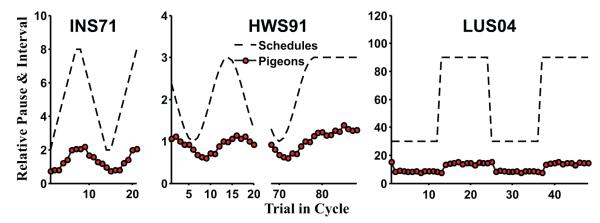
Interval cycles and sample data from the three experiments modeled in this paper: INS71 (Innis and Staddon, 1971), HWS91 (Higa et al., 1991), and LUS04 (Ludvig and Staddon, 2004).

A second challenging feature of these cyclic-interval schedules is that the data often fail to exhibit the timescale invariance typical of interval timing on static schedules (e.g., Gallistel and Gibbon, 2000) though not universally (see Zeiler and Powell, 1994; Ludvig et al., 2008; Kehoe et al., 2009). With static schedules, for example, doubling the to-be-timed interval will usually result in timed responses that are both twice as long and twice as variable (e.g., Schneider, 1969; Gibbon, 1977). On dynamic schedules, in contrast, longer intervals often elicit proportionally shorter pauses (e.g., Innis and Staddon, 1971; Higa et al., 1991; Ludvig and Staddon, 2004, 2005). The right panel of Fig. 1 illustrates how, on cyclic schedules, when the interval varies across a threefold range (from 30 to 90 s) the post-reinforcement pause less than doubles. This dependence of response timing on the absolute timescale poses a second challenge for timing theories.

One newly developed timing theory seems particularly well-suited to deal with these timing dynamics because of its ability to learn rapidly: the time-adaptive drift-diffusion models (TDDMs; Rivest and Bengio, 2011; Simen et al., 2011). Basic drift-diffusion models (DDMs) are the most widely used process model of real-time decision making (Ratcliff, 1978; Ratcliff and Rouder, 2000). In a DDM, decisions are made by accumulating noisy evidence (modeled as a random walk with drift) until a threshold is reached, eliciting a response. One strength of this class of models is that they assume variability within trials in several components of processing, making it possible to study those components in isolation and to make real-time predictions. These features make DDMs particularly well suited to model both measures of accuracy and response-time distributions (Ratcliff, 2002; Ratcliff and McKoon, 2008; Leite and Ratcliff, 2010). Moreover, strikingly, noisy ramping neural activity that matches the noisy evidence accumulation process in a DDM can be seen in certain cortical areas during decision-making tasks (Bogacz, 2007; Gold and Shadlen, 2007; Rushworth et al., 2011). As noted by Leon and Shadlen (2003), this activity shares some properties with interval timing and could be a potential neural substrate for timing in monkeys.

Recently, two similar formal extensions of this DDM framework to interval timing were introduced: the adaptive drift-diffusion process (ADDP, Rivest and Bengio, 2011) and the stochastic ramp and trigger (SRT, Simen et al., 2011). Though independently developed, the ADDP and the Level-4 SRT models are almost identical, and we refer to them by the joint name of TDDMs (time-adaptive DDMs). Both models extend the DDM by incorporating a learning rule that allows for rapid adaptation of the drift rate to the experienced time interval. These TDDMs can even adapt to a change in experienced time intervals as rapidly as a single trial. One potential limitation of these TDDMs, however, is that timescale invariance is built right into the algorithm. As a result, whether these models can account for dynamic timing data, which often lack such invariance, is unclear.

In the TDDMs, the memory of recent intervals is stored in the drift rate, which controls the slope of the signal over time. A change in the experienced intervals leads to a change in the drift rate (i.e., the accumulator slope). Interestingly, a similar change in the slope of the firing rate of neurons has been observed during timing tasks in the posterior thalamic region in rats (Komura et al., 2001) and multiple cortical areas in monkeys (Leon and Shadlen, 2003; Reutimann et al., 2004; Lebedev et al., 2008). The TDDMs have also been shown to be a reasonable approximation of more complex networks of spiking neurons (Simen et al., 2011).

In the timing literature, the only major model that explicitly contends with interval timing dynamics is the multiple-time-scale (MTS) habituation model (Staddon and Higa, 1999; Staddon et al., 2002). The MTS model uses a decaying memory trace to keep track of time. This memory trace is made up of a sum of decaying units that increases in activity when a reward is presented. A response threshold is updated at every trial to correspond to the level of decay in the memory trace at the moment the reward was last seen. This dynamic threshold enables MTS to reproduce the tracking behavior observed in cyclic schedules such as those shown in Fig. 1.

In this paper, we systematically compare the performance of the TDDMs and MTS on three different sets of dynamic timing data in pigeons from the published literature (Innis and Staddon, 1971; Higa et al., 1991; Ludvig and Staddon, 2004). These datasets use different cyclic-interval schedules and are fairly representative of the literature on the dynamics of interval timing. Because of the dependence on absolute timescales in the timing measures, MTS is able to better match the pigeon data than the basic TDDM models. Motivated by this shortcoming of the basic TDDM, we introduce a modified TDDM with a threshold that depends linearly on the slope of the drift rate (the LT-TDDM). This modified TDDM matches the timing data from pigeons as well as or better than MTS in most experiments.

2. Methods

2.1. Model specifications

2.1.1. Time-adapting drift-diffusion model (TDDM)

A drift-diffusion process consists of a noisy signal randomly drifting over time but tending toward a particular direction as dictated by its drift rate. In the TDDM implementation, this signal φ(t) starts at 0 at stimulus onset, and thus serves as the internal representation of elapsed time t from stimulus onset. This drifting process is analogous to an accumulator that continuously integrates time at a drift rate w with noise ε(t):

$$\phi \left(t\right)=\phi (t-1)+w\Delta t+\epsilon \left(t\right)$$ (1)

where Δt is the time step used to simulate the continuous process and ε(t) is Gaussian noise with mean 0 and variance σ² [N(0, σ²)]. On reward, the signal φ(t) is reset to 0. The signal has an upper absorbing boundary at 1, meaning that once φ(t) reaches 1, it stays there until reset by a reward. To achieve Weber’s law, whereby the variance in responding is proportional to the mean (Gibbon, 1977), the noise variance σ² must equal β²wΔt (Rivest and Bengio, 2011; Simen et al., 2011). In the model, responding begins when the accumulated signal φ(t) exceeds a threshold θ. The signal is constrained to 0 ≤ φ(t) ≤ 1. Although usually written in differential-equation form, the DDM is described here as difference equations for ease of comparison with the MTS model (for the continuous time formulation, see Rivest and Bengio, 2011; or Simen et al., 2011).

Learning in the model occurs by adapting the drift rate w through two rules. First, when the reward occurs before the signal φ(t) has reached 1, the change Δw(n), following trial n, in drift rate w, is calculated based on the ratio between the distance to the target accumulated signal (a value of 1) and the actual accumulated signal (φ(t)):

$$\Delta w\left(n\right)=w\left(n\right)\frac{(1-\phi (t\left)\right)}{\phi \left(t\right)}$$ (2)

Fig. 2 illustrates geometrically why this update equation leads to the appropriate change in the drift rate. This change is tantamount to a positive prediction error signal that drives the drift rate higher. If, however, the signal φ(t) reaches its boundary before the reward occurs, then the drift rate w is slated to decrease. The rate change for that trial Δw(n) is cumulated until the next reward occurs:

$$\Delta w(n,t)=\Delta w(n,t-1)-{\left(w\right(n)+\Delta w(n,t-1\left)\right)}^2\Delta t$$ (3)

where Δt is a small time step size used to simulate the continuous process. Independently of whether rule (2) or (3) is engaged on a particular trial n, only a fraction of the change Δw(n) is applied to w at the time of reward using a learning rate α:

$$w(n+1)=w\left(n\right)+\alpha \Delta w\left(n\right)$$ (4)

This way, the drift rate w tracks the reward rate (Rivest and Bengio, 2011), similar to the manner in which the pacemaker rate is tied to the reward rate in BeT (Killeen and Fetterman, 1988).

Fig. 2.

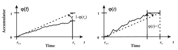
A geometric illustration of the principle behind the TDDM learning rules. Left: When the reward occurs earlier than expected, the drift rate w is corrected toward the correct rate of the observed interval by rules (2) and (4), increasing the slope of the accumulator. Right: When the accumulator reaches its maximum boundary, the drift rate w is slowly decayed toward rate of the observed interval through rules (3) and (4), decreasing the slope of the accumulator.

The TDDM model is fully defined by 3 parameters: α, β and θ. The learning rate 0 ≤ α ≤ 1 determines how quickly w adapts to the observed intervals. Because α is constant, the drift rate is an exponential-moving average of the reward rate. The noise factor β ≥ 0 corresponds to the timing precision in proportion to the interval encoded by 1/w. The threshold 0≤θ≤1 corresponds to the proportion of the time interval encoded by 1/w before response onset. Together, the drift rate w and threshold θ determine the expected post-reinforcement pause for a given trial in the model.

2.1.2. An alternative TDDM learning rule

The TDDM, as presented in Eqs. (2)–(4), uses a learning rule which converges to the reward rate—equivalent to the harmonic mean of observed intervals (ADDP, Rivest and Bengio, 2011). A very similar rule, independently developed, was also recently introduced as a potential model of interval timing (SRT, Simen et al., 2011). Although the two formulations are exactly equivalent when α = 1 (single-trial learning), when α < 1, the decay processes are different (Eqs. (3) and (5)). In the SRT level-4 model, the decay is directly applied with a learning rate:

$$w\left(t\right)=w(t-1)-\alpha w{(t-1)}^2\Delta t$$ (5)

instead of being cumulated as in (3) and (4). This equation pushes 1/w toward the arithmetic mean instead of the harmonic mean of the observed intervals (Rivest and Bengio, 2011). This divergence in fixed point may lead to different results because the harmonic mean is smaller than the arithmetic mean for non-equal positive numbers.

2.1.3. Linear threshold TDDM (LT-TDDM)

The TDDMs are almost perfectly timescale invariant when the learning rate is near 1, yet the empirical data from dynamic timing seems not to be (see Fig. 1). Thus, one key question in the simulations is whether TDDMs with a lower learning rate can accommodate the timescale dependencies apparent in the pigeon data.

As a potential alternate approach to reconciling TDDMs with these data, we developed a linearized version of the TDDM (LT-TDDM), where the threshold θ is now replaced by a linear function of the event rate encoded in w:

$$\theta =a+\mathit{bw}$$ (6)

This version allows the model additional flexibility to deal with changes in behavior that are linearly related to the timescale. To obtain an estimate of the post-reinforcement pause from the threshold we divide Eq. (6) by the slope w of the temporal integrator:

$$t_{\text{pause}}=\frac{a}{w}+b$$ (7)

There are now two parameters, a and b, replacing θ, so the LT-TDDM has a total of 4 parameters: α, β, a, and b. The parameter a is equivalent to the threshold in the original formulation (anticipation) and represents a proportion of the encoded interval. The parameter b corresponds to the addition of a constant, baseline pause, independent of the interval encoded or the timescale, as shown in Eq. (7). This fixed delay is analogous to the switch closure time in the information-processing elaborations of SET (e.g., Gibbon et al., 1984). In this paper, we used the harmonic mean (Eqs. (2)–(4)) version of TDDM (Rivest and Bengio, 2011)] in LT-TDDM, but the extension could be applied to both TDDMs and possibly to other accumulator-based timing models that use a fixed threshold (e.g., SET, Gibbon, 1977).

2.1.4. MTS model

The multiple-time-scale (MTS) model (Staddon and Higa, 1999) is based on the idea that time is encoded as the strength of a memory trace. This trace is stored in the activity of a cascade of leaky integrators V_j of the form:

$$V_j\left(t\right)=a_j{V}_j(t-1)+b_{\mathit{MTS}}{X}_j\left(t\right)$$ (8)

where 0 < a_j < 1 is a decay constant and b_MTS > 0 is the stimulus weight, X_j is the stimulus, and t is the discrete time step. For a system with M integrators, the memory trace v is given by the sum of the activity of all integrators:

$$v\left(t\right)=\sum _{i=1}^M{V}_i\left(t\right)$$ (9)

The external stimulus X₁(t) is set to 1 for one time step at reward onset and is zero otherwise, while the stimulus for the jth integrator for j > 1 is defined by:

$$X_j\left(t\right)=\{\begin{array}{cc}{X}_{j-1}\left(t\right)-V_{j-1}\left(t\right)\hfill & \text{if}{X}_{j-1}\left(t\right)>0\hfill \\ 0\hfill & \text{otherwise}\hfill \end{array}\phantom{\}}$$ (10)

The integrators are ordered in the cascade according to their decay constants a_j = 1 − e^−λj. The shape of the trace v(t) depends on the reinforcement history of the system. For example, after training on a fixed-interval schedule, v(t) eventually becomes a periodic function of time.

This trace is transformed into a timing mechanism by triggering responses whenever the trace falls below a threshold value. The threshold θ is set for every trial n by:

$$\theta \left(n\right)=v(n-1)+\xi X\left(n\right)+\eta \epsilon \left(n\right)$$ (11)

where v(n − 1) is the value of the trace in the previous trial just before reinforcement, X(n) is the reinforcement magnitude (always 1) that begins the current trial, ε(n) is a noise term with uniform distribution ranging from −0.5 to 0.5 [U(−0.5,0.5)] and ξ and η are constants (Staddon et al., 2002). In total, MTS has five free parameters: M, λ, b_MTS, and η.

2.2. Simulated datasets

2.2.1. Innis and Staddon (1971) dataset (INS71)

The first dataset comes from Experiment 1 in Innis and Staddon (1971). Fig. 1 (left panel) shows how the experiment consisted of 5 linearly ascending and descending interval durations of the form:

$${\mathit{IFI}}_{\mathrm{asc}}=(2S,3S,\dots ,8S)\text{and}{\mathit{IFI}}_{\text{desc}}=(8S,7S,\dots ,2S)$$ (12)

where S ∈ {2.26, 4, 10, 20, 40}. The original experiment had 10 sessions, each with four cycles of 14 trials, as did our simulations. Only the data from the average of the last three cycles (42 trials) in each of the last five sessions were used (15 samples per trial point). Simulations were conducted with the same protocol. In the models, pause duration was taken to be the time until first threshold crossing, even if this exceeded the interval duration. The pigeon data (mean pause times for each point in the cycle) used for fitting was extracted with the aid of a ruler directly from Fig. 1 (right panel) in the original paper. Because data for each individual was not available, the models were fit to the population average.

2.2.2. Higa et al. (1991) dataset (HWS91)

The second dataset comes from Experiment 1 in Higa et al. (1991). Fig. 1 (middle panel) shows how the experiment consisted of interval durations that varied sinusoidally according to:

$$\mathit{IFI}\left(n\right)=S\left(2+\sin \left(\frac{2\pi n}{8}\right)\right)$$ (13)

where S ∈ {5,30} for between 1 and 5.25 cycles per session. Each session was 100 trials long and ended with the longest interval for at least 16 consecutive trials. The experiment lasted 20 sessions. Only the last 16 sinusoidal trials and the first 16 long constant trials were used for analysis (20 samples per trial point). Simulations were conducted with the same protocol. In the models, pause duration was taken to be the time until first threshold crossing, even if this exceeded the interval duration. The pigeon data (mean pause times for each point in the cycle) were extracted directly from Fig. 5 in the original paper with the aid of a ruler. Because separate data for each pigeon was available, the models were fit to each pigeon individually.

Fig. 5.

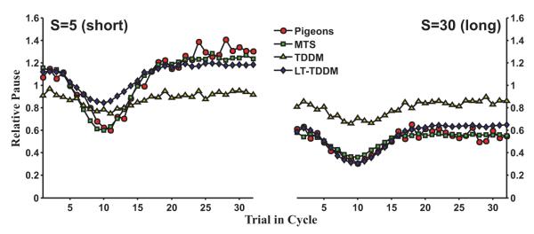
Best mean fits for MTS, TDDM, and LT-TDDM plotted with the mean pigeon data in the HWS91 experiment (Higa et al., 1991, Fig. 5). The TDDM remains approximately timescale invariant and cannot fit the timescale changes across conditions. Both MTS and the LT-TDDM are better fits, but MTS provides a noticeably better match on the shorter time scale (S = 5).

2.2.3. Ludvig and Staddon (2004) dataset (LUS04)

The third dataset was drawn from Experiment 1 in Ludvig and Staddon (2004). Pigeons were presented with alternating blocks of 30-s and 90-s intervals (see Fig. 1, right panel). Six schedules, with different numbers of 30-s and 90-s intervals in each block, were used. A simulation consisted of a number of sessions (as listed in Ludvig and Staddon, 2004, Table 1), and each session had 100 trials. Only the last 5 sessions were used for analysis, and the first four intervals of each session were excluded. Simulations were conducted with the same protocol. Pause duration in the models was taken to be the time until first threshold crossing, even if this exceeded the interval duration. The mean empirical pause durations were recalculated from the original pigeon data and were used to fit each model to each pigeon individually. In calculating the mean pauses for the pigeon data, pauses that exceeded by 30 s after the longer criterion were considered outliers (0.07% of trials) and excluded, as per the original empirical paper (Ludvig and Staddon, 2004).

Table 1.

MTS and LT-TDDM correlations with pigeon’s data with and without a lag of 1. Standard deviations are estimated using the 10 simulations for each model. MTS is lagging.

S	MTS		LT-TDDM
	No lag	Lag 1	No lag	Lag 1
2	0.82 ± 0.01	0.97 ± 0.00	0.97 ± 0.01	0.94 ± 0.01
4	0.80 ± 0.01	0.96 ± 0.00	0.96 ± 0.00	0.94 ± 0.01
10	0.84 ± 0.01	0.96 ± 0.01	0.96 ± 0.00	0.91 ± 0.00
20	0.88 ± 0.01	0.94 ± 0.01	0.95 ± 0.01	0.85 ± 0.01
40	0.83 ± 0.02	0.93 ± 0.01	0.90 ± 0.01	0.91 ± 0.01

As a further test of the models, one dataset from Experiment 3 in the same paper was also used (Ludvig and Staddon, 2004, Experiment 3C). In this experiment, pigeons were presented with alternating blocks of 60-s intervals and 180-s intervals. Unlike the earlier simulations, these simulations, however, did not find new parameters that provided the best fit to these data. Simulations were run with the same parameters that were found by fitting the pigeon data in Experiment 1. This approach provides a robust test as to whether the models generalize to the new conditions of Experiment 3 without any additional parameters. Simulations followed the same protocol as the simulations of Experiment 1 and were run for 9 sessions of 100 trials.

2.3. Fitting procedure

To evaluate the quality of the model fit to the animal data, the best possible parameters for each model to fit each pigeon were selected in a two-step process. First, a grid search in parameter space was conducted. The best point from this search was then used as a seed for a gradient optimization of that parameter, using the fmincon function (with the active-set algorithm) in MATLAB (Optimization Toolbox, Mathworks, Natick, MA) to minimize the log mean squared error. In the grid search, ten simulations were run for each point in parameter space. All simulations were run with a time step (Δt) of 100 ms, matching the standard description of MTS, and being small enough to simulate the TDDMs on the given tasks. In the grid search, for MTS, every possible combination of M (number of units) in the range [5, 15], λ (decay) and b_MTS (injection) logarithmically spaced in range [10⁻², 10^1/2], ξ ∈ {0.10, 0.14, 0.20} (learning), and η ∈ {0.02, 0.04, 0.06, 0.10} (noise), were evaluated, for a total of 3960 possible parameter combinations. For both TDDMs, the grid search evaluated α (learning rate) logarithmically spaced in range [10⁻², 1], β (precision) linearly spaced in range [0.05, 0.25], and θ linearly spaced in range [0.05, 1.00] for a total of 6000 possible combinations.

Fitting the LT-TDDM requires an extra dimension in the grid search, making this parameter search computationally an order of magnitude more demanding than the equivalent search for the TDDMs. In the TDDMs, changing the threshold has only a limited effect on the time encoded in the drift rate w because the observed delays are identical so long as a response is emitted within the interval (independent of when). To take advantage of this relative independence of parameters, the results from most of the 200 TDDM simulations from the ADDP version (Rivest and Bengio, 2011) having the same (α, β, θ) triplets were grouped together. Using these groupings, initial values for a and b were then estimated using linear regression to find the two parameters that best aligned the TDDM simulations to the animal data. Those parameters were used as the initial a and b on a grid search to find the best (α, β) for LT-TDDM. A gradient descent search starting on that initial quartet (α, β, a, b) was then run using the same method as the other models.

Models were compared using the AICc measure (Akaike Information Criterion with a correction). This measure is a corrected version of AIC that is less biased than the original form (Akaike, 1974), especially for small sample size N or ratio of sample size to parameters N/K < 40, and thus, should be preferred (Burnham and Anderson, 2002). The AICc compares the relative goodness of fit of the models, but penalizes those models with more parameters. Goodness of fit is measured by the squared error of post-reinforcement pauses between simulation data and animal data in time-scaled units:

$$\mathrm{AICc}=N\log \left(\frac{{\Vert \text{Model}-\text{Data}\Vert }_2^2}{N}\right)+2K+\frac{2K(K+1)}{N-K-1}$$ (14)

combined with a correction based on K and N, where N is the total number of intervals used to compare model against data in a given experiment (70 in INS71, 64 in HWS91, and 82 in LUS04) and K is the number of free parameters (K = 5 for MTS, 3 for TDDMs, and 4 for LT-TDDM). The absolute scale of the AICc scores is irrelevant—only the differences between models are meaningful (ΔAICc). Thus, we rescaled the AICc scores by subtracting the AICc score of the model with the lowest score from all the other models. With this rescaling, the best model always had a ΔAICc of 0, and the other models had positive scores, with larger numbers indicating less support for the model. As a rule of thumb, ΔAICc scores <2 mean strong support for that model, while ΔAICc scores >10 mean virtually no support for that model (Burnham and Anderson, 2002).

In the optimization procedures, the difference between the simulated and empirical data was rescaled so that the error was proportional to the schedule’s timescale. This rescaling was necessary so that the optimization algorithm would not put more weight on fitting the longer timescale experiments, which have larger absolute errors, over the shorter ones. The log mean squared error and AICc scores were always averaged over 10 runs. The set of parameters with the best (lowest) log mean squared error was selected and AICc scores reported for that point.

3. Results

3.1. Simulation of INS71

In the INS71 dataset, pigeons tracked a linearly ascending and descending sequence of intervals (Fig. 1, left panel). Fig. 3 depicts how all three models produce reasonable approximations of this temporal tracking behavior, which looks nearly timescale invariant across the different schedules (S ranging from 2.26 to 40). Fig. 4 (left panel) shows that the LT-TDDM had the lowest AICc score with other three models nearly 30 points behind (very weak support for those models). As can be seen in Fig. 3, the TDDM and LT-TDDM look more in phase with the pigeon data than MTS. To validate this observation, the cross-covariance between the pigeon data and the data for each model were computed with different phase shifts. MTS pauses had a consistently higher co-variance to pigeon pauses when shifted left by 1 trial, except on S = 20 where they were almost equal. For all the TDDM-based models, the covariance with the pigeon data was higher without any phase shift of the trials. Correlations for the MTS and LT-TDDM models with and without a lag of 1 are shown in Table 1. The MTS simulations are consistently more correlated with the pigeon data when shifted left by one trial. This visual difference was borne out in the statistical measure of model quality (see Fig. 4). Overall, on this dataset, LT-TDDM was the strongest match, followed by both TDDMs, and finally the MTS model, because the model lags behind the pigeon data.

Fig. 3.

Best mean fits for MTS, TDDM, and LT-TDDM plotted with the pigeon data in the INS71 experiment (Innis and Staddon, 1971, Fig. 1). LT-TDDM provides a clearly better fit than the other two models. TDDM and LT-TDDM are also more in phase with the animal’s behavior while MTS lags behind by about one trial.

Fig. 4.

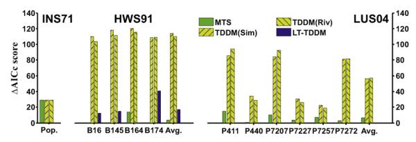
ΔAICc scores for all four models on all three experiments for each individual pigeon. ΔAICc is the difference in AICc score with the best model for a given fit. Lower is better (in each case, the best model has ΔAICc = 0). The final set of bars in each panel are the model ΔAICc scores averaged over all pigeons in that experiment.

The best parameters for each model when fitted to the population average are given in Appendix. The best MTS parameters were very similar to those used in other papers on the model (e.g., Staddon et al., 2002). For both TDDMs, the learning rate was 1 (single-trial learning), and the response threshold was set at 28% of the estimated interval. For the LT-TDDM, the threshold was 24% of the estimated interval plus a 1.3 s fixed pause (b = 0 would be close to timescale invariant). Noise levels were low in every model, but the noise could not really be fitted in the absence of information about variability in responding, which was not available for that dataset.

3.2. Simulation of HWS91

In this dataset, pigeons tracked a sinusoidal sequence of intervals (Fig. 1, middle panel). Models were fitted and evaluated for each pigeon individually. Individual AICc results are shown in Fig. 4 (middle panel). MTS has the best score for all pigeons except B164 (where LT-TDDM did better by 14 points) followed closely by LT-TDDM. Fig. 5 shows that both MTS and LT-TDDM were able to reproduce this behavior very well. MTS was slightly superior, in particular with the shorter timescale (S = 5), whereas the TDDMs performed considerably worse than the other two models (ΔAICc > 100; see Fig. 4).

The TDDMs struggled to deal with the lack of timescale invariance across schedules (S from 5 to 30) in the animal data. If the data were timescale invariant across schedules, both plots in Fig. 5 should overlap, as they do for the TDDMs (see Fig. 5). To match the data on both timescales, the TDDMs were forced to an averaged trend line with little amplitude in the adaptation to recent intervals. Comparing the two learning rules, TDDM (Riv) did slightly better than TDDM (Sim) on every fit by an average of 6 points per data set. The LT-TDDM was not able to match the full dip in pausing with the short time-scale schedule (S = 5, Fig. 5 left panel), but does effectively deal with the timescale change across schedules. Overall, the LT-TDDM matched the data much better than the TDDMs, but somewhat worse than MTS (mean ΔAICc = 14 for LT-TDDM worse than MTS).

The best model parameters for each pigeon dataset are given in Appendix. The best MTS parameters were very similar again to what has been used in other papers on the model (e.g., Staddon et al., 2002) with slightly higher λs. The TDDMs have a much lower learning rate (around 0.01 (Riv) and 0.15 (Sim)), explaining why the TDDMs hardly track the changing intervals in Fig. 5. The thresholds for the TDDMs were all higher than in the INS71 simulation, ranging from 30% to 52% (as opposed to 28% for the population data in INS71). The LT-TDDM learning rates averaged ≈0.5, and the threshold parameters a and b averaged 0.18 and 3.2 respectively, meaning that, on average, the threshold was about 18% of interval duration plus 3.2 s of constant pause. Noise levels were higher than in INS71 for every model in almost every fit except LT-TDDM. The noise, while not used to fit the individual pigeons’ variability (which was not available), does push the harmonic mean downward since the harmonic mean is lower than the arithmetic mean.

3.3. Simulation of LUS04

In this dataset, pigeons tracked a square-wave sequence of intervals as depicted in the right panel of Fig. 1. Models were fitted to the mean pause times and evaluated for each individual pigeon (Ludvig and Staddon, 2004). Fig. 4 (right panel) shows how, based on the AICc scores, the LT-TDDM was best at fitting every single pigeon of the population (ΔAICc was always 0), with MTS second (mean ΔAICc = 6), and the TDDMs far behind (mean ΔAICc scores of 56 and 57). The two variations on the TDDM have similar scores with no clear best model on this dataset.

Fig. 6 illustrates how, even within a single condition, the animal data is not timescale invariant. Whereas the difference between the two intervals (30 s and 90 s) is threefold, the range of pauses in the pigeon data is at most twofold (e.g., Fig. 6, left-most panel) or even less. The TDDMs, with a low learning rate (mean = 0.07 and 0.09), do exhibit this lack of timescale invariance, but at the cost of slow transitions following a sudden change in the observed intervals. Pigeons, on the other hand, showed rapid transitions in their pauses with almost no gradual adaptation (most evident in the rightmost panels of Fig. 6). Any residual adaptation occurs mainly when shifting from short to long intervals and is relatively small compared to the initial increase. The TDDMs clearly take too long to adapt, whereas MTS and the LT-TDDM, both show a major adaptation on the first trial following a change in interval and further increases following the second and third long intervals, similar to the pigeon data. On this dataset, MTS and the LT-TDDM are hard to discriminate from each other on the averaged plot.

Fig. 6.

Best mean fits for MTS, TDDM, and LT-TDDM plotted with the mean pigeon data on the 6 square-wave schedules in the LUS04 dataset (Ludvig and Staddon, 2004). The TDDM adapts more slowly than the pigeons, whereas MTS and LT-TDDM are fairly close.

To better evaluate how well these modeling results generalize beyond the datasets for which the parameters were optimized, we ran an extra simulation using 12 intervals of 60 s and 180 s instead of 30 s and 90 s. This new simulation also highlights the ability of the different models to generalize, or extrapolate, to a longer timescale. Each model was run on this new schedule with the parameter values found to fit data from LUS04 Experiment 1. The simulated results for each individual pigeon were then averaged and compared to the population average from Experiment 3 of Ludvig and Staddon (2004). In that experiment, the same pigeons as in the LUS04 dataset received a square-wave schedule with blocks of 12 60-s intervals alternating with blocks of 12 180-s intervals.

Empirically, pigeons paused on average 15.0 s after the 60-s intervals and 21.1 s after the 180-s intervals (Ludvig and Staddon, 2004, Table 3). Fig. 7 shows the model predictions from the simulations. The TDDMs fail at predicting both the short and the long pauses. MTS does poorly at predicting the pause after long intervals (17.5 s), but predicts the pause after short intervals (14.9 s). The LT-TDDM predicts both pauses pretty well (13.9 s after short intervals and 22.8 s after long intervals). The generalizability of LT-TDDM to interval durations with which it has not been trained on is strong evidence of the model’s potential utility. Note that these simulations used the parameters derived from fitting the models to the LUS04 dataset (hence AICc analysis does not apply) that only has 30-s and 90-s intervals, thus pushing these simulations beyond basic curve fitting. In addition, extrapolation is much more difficult than interpolation because there is no data to train or fit the system for that region of the problem space to interpolate a result. To properly extrapolate, a model must have the appropriate internal representation to make reliable predictions outside the range of its training or calibration set.

Fig. 7.

The model-predicted post-reinforcement pauses for the 12 × 60 12 × 180 square-wave schedule plotted with the mean pigeon data (Ludvig and Staddon, 2004). Only the LT-TDDM provides a good match to the data in this extrapolation test.

The best parameters for each model are listed in Appendix. The best MTS parameters were very similar to previous ones, except b_MTS and noise level η which were much higher, likely explaining the rapid adaptation of MTS in this dataset. Using a more standard value of b_MTS generates slower transitions, more similar to the slow adaptation of the TDDMs. There is a large difference in the learning rates between the TDDMs (mean = 0.09) and LT-TDDM (mean = 0.89). LT-TDDM has a much higher learning rate, explaining its sharper transition when a new interval is observed. The threshold hovers around 26% of the interval for TDDMs, meaning that the model waits on average 26% of the interval encoded by 1/w. The LT-TDDM has an averaged threshold representing 8% of the encoded interval plus about 9.1 s of constant pause. This linear threshold, with a constant pause component, not only allows LT-TDDM to better fit the lack of time-scale invariance within the set of schedules from LUS04 Experiment 1, but also allows LT-TDDM to predict the post-reinforcement pause on an unseen timescale twice as large (the 12 × 60 12 × 180 task) in Experiment 3 (Ludvig and Staddon, 2004).

4. Discussion

Overall, across the 3 experimental datasets, the LT-TDDM most closely approximated pigeon timing behavior. Fig. 4 presents a summary of the AICc scores for the different experiments. The TDDMs (Rivest and Bengio, 2011; Simen et al., 2011), despite displaying some tracking and timescale dependence, consistently failed to reproduce the key features of these behavioral datasets. The MTS model, which was designed in part to deal with these timing dynamics (Staddon and Higa, 1999), fitted the data from the HWS91 dataset better than the LT-TDDM, but was significantly worse for the other two datasets (most notably in the lag on the INS71 dataset). In addition, when the models were tested for their extrapolation capacity on a novel timescale and dataset, LT-TDDM better approximated the pigeon behavior than MTS (Fig. 7). The MTS model, however, did match the data better than the standard TDDMs almost across the board.

Although the LT-TDDM could not account for all aspects of the data, on the whole this model provided the best results out of the four models examined, followed closely by MTS. These models represent the only models that, as far as we know, have been explored as potential computational models of interval timing dynamics. The threshold modification mechanism in the LT-TDDM suggests that dealing with these dynamics requires a flexible threshold in an accumulator-type model, such as the TDDMs simulated here, or even in more traditional timing theories such as SET (Gibbon, 1977) and BeT (Killeen and Fetterman, 1988). As shown on the square-wave schedules, this mechanism allowed for a rapid adaptation and a dependence on the absolute timescale both across (Figs. 3 and 5) and within (Fig. 6) schedules.

4.1. Choosing a threshold for timing

One consistent feature of these three datasets on timing dynamics is that they are not strictly timescale invariant. This pattern stands in contrast to what is commonly observed with static timing procedures (Gallistel and Gibbon, 2000). For example, in Fig. 1, the interval varies threefold between the shortest and longest interval, but the pause only doubles. If the pigeon data were timescale invariant, then the pause would triple over that range, and the two time-scaled graphs would superimpose. The basic TDDMs, however, have strict timescale invariance built directly into the timing mechanism (Rivest and Bengio, 2011; Simen et al., 2011), which can only be circumvented through a low learning rate. As a result, the basic TDDMs should (and do) struggle to fit the lack of invariance and fast adaptation observed in these datasets. The use of the harmonic mean, when learning time intervals, could also have helped, because it biases the time encoded downward. Whereas the harmonic mean version of the TDDM is slightly better, that variation is still insufficient and far inferior to MTS and the LT-TDDM.

Introducing, however, what would seem to be a small change in the TDDM architecture—allowing the threshold to depend on the drift rate—was sufficient to get much better fits in the experiments evaluated here. This factor is formally equivalent to adding a constant pause, independent of the observed intervals, and is analogous to the switch closure time in SET (e.g., Gibbon et al., 1984). The LT-TDDM results suggest that, if the TDDM is a good representation of the underlying timing process, then the pause is determined by at least two components: a time-scaled component perhaps related to the anticipation of the upcoming interval and an additional constant pause, which may be due to non-timing factors, such as attention or motivation (Lowe et al., 1974; Ludvig et al., 2007; Galtress et al., 2012). This addition in the LT-TDDM can still preserve the time-scale invariance of the basic TDDM because setting the constant b to 0 removes this extra pause and reduces LT-TDDM to the basic TDDM.

A similar event-rate dependent threshold could also be adapted to other timing models. Both SET and BeT count the ticks of a pacemaker to mark the passage of time (Gibbon, 1977; Gibbon et al., 1984; Killeen and Fetterman, 1988). To time different interval durations, SET adjusts the threshold while keeping the tick rate constant, whereas BeT keeps the threshold constant while adjusting the tick rate (faster for shorter intervals and slower for longer). If, instead of the drift rate, we interpret w as tick rate then the same LT-TDDM threshold could be equally employed by BeT (see also Simen et al., 2011). Similarly, the SET threshold is usually defined as:

$$\frac{t^{\ast }-t}{t^{\ast }}<\theta$$ (14)

which can also be expressed as θ = at* where 0 < a < 1, t is the number of ticks and t* is the number of ticks at reinforcement. Because this threshold is already dependent on the interval duration, modifying it accordingly would simply require that a constant be added, such that θ = at* + b. These modifications would allow both SET and BeT to account for one feature of these datasets: the lack of timescale invariance. The tracking in the cyclic schedules would require the introduction of additional learning rules to those models, which is beyond the scope of the current work. Future work may elucidate what modifications might be required to align these models with the data on the dynamics of interval timing.

4.2. Model limitations

Perhaps the biggest challenge facing the basic TDDMs and the LT-TDDM in their current formulation lies in explaining a classic static timing task called the peak procedure (Catania, 1970; Roberts, 1981). In the peak procedure, on most trials, food reward becomes available after a fixed time, but occasional probe trials are interspersed where food is not delivered. None of the TDDMs have a mechanism to stop accumulating evidence if reward is not presented at the expected time. As a result, following a probe trial, the drift rate should decay down toward zero, and the model should respond late, or not at all, on the next trial. One remedy would be to constrain the updates (Eqs. (3) and (5)) to only occur if a reward occurs within a maximum delay after the expected timing or only if that trial is rewarded.

In addition, during peak trials, animals eventually stop responding after the criterion interval duration has elapsed. Both the LT-TDDM and MTS could potentially be adapted to accommodate this data by adding a second threshold that would trigger the end of responding. But how this stop threshold would appear during training remains undefined. Alternatively, for the LT-TDDM, the termination of responding could perhaps be implemented by a second diffusion process, which controls the inhibition of behavior. This process could be initiated at trial onset with the primary diffusion process, or when the latter hits and sticks at the upper absorbing boundary. It is not clear, however, whether these changes would produce responding that matches the distribution of stop times (Church et al., 1994; Balci et al., 2009). But given the similarity of start times in fixed-interval schedule and the peak-interval procedure, all the TDDMs should still reproduce the start time appropriately.

4.3. Conclusion

In brief, we found that, although the TDDMs were developed to account for both timescale invariance and rapid adaptation to changing intervals as observed in animals (Rivest and Bengio, 2011; Simen et al., 2011), the basic models do not match the data under cyclic schedules as well as the MTS model does (Staddon and Higa, 1999). In this paper, we showed that by simply making the TDDM threshold a linear function of its drift rate, we were able to reconcile both fast adaption and a lack of timescale invariance without sacrificing model performance in other areas.

This new threshold assumes that the pause is driven by two distinct factors: a constant, reactive component plus a proportion of the anticipated interval. Because a low learning rate alone was insufficient to explain the timescale dependencies in these datasets, our result suggests that other accumulator-based models, such as SET and BeT, might also require a similar constant element if an adaptive version of these models were to be developed. Based on the principles behind the firmly established DDMs (Ratcliff, 1978, 2002; Ratcliff and McKoon, 2008; Bogacz, 2007; Gold and Shadlen, 2007; Leite and Ratcliff, 2010; Rivest and Bengio, 2011; Simen et al., 2011), the LT-TDDM includes the important static features behind SET and BeT while also successfully reproducing the timescale-dependent rapid adaptation observed on dynamic timing schedules.

Appendix

See Appendix Tables A1–A3.

Table A1.

MTS best parameters for each fit.

Dataset/pigeon	M	λ	bMTS	ξ	η
INS71/Pop.	13	0.6781	0.0418	0.1378	0.0226
HWS91/B16	10	0.6859	0.0450	0.1018	0.0392
HWS91/B145	9	0.7496	0.0422	0.1000	0.0400
HWS91/B164	10	0.7302	0.0410	0.0972	0.0254
HWS91/B174	10	0.7495	0.0422	0.1000	0.0200
LUS04/P411	10	0.6690	0.0444	0.1000	0.0991
LUS04/P440	9	0.6749	0.1782	0.2000	0.1000
LUS04/P7207	8	0.7478	0.1777	0.1926	0.0957
LUS04/P7227	11	0.6726	0.0415	0.1388	0.1000
LUS04/P7257	10	0.7430	0.0415	0.1397	0.0197
LUS04/P7272	7	0.6767	0.7507	0.1999	0.1000

Table A2.

TDDMs best parameters for each fit.

Dataset/pigeon	TDDM (Riv)			TDDM (Sim)
	α	β	θ	α	β	θ
INS71/Pop.	1.0000	0.0441	0.2834	1.0000	0.0441	0.2834
HWS91/B16	0.0100	0.1952	0.4627	0.2527	0.2014	0.3063
HWS91/B145	0.0110	0.1501	0.4006	0.1130	0.1999	0.3000
HWS91/B164	0.0100	0.1999	0.5173	0.1865	0.1468	0.3529
HWS91/B174	0.4828	0.1488	0.3499	0.4912	0.2008	0.3603
LUS04/P411	0.0845	0.0932	0.0285	0.0960	0.0524	0.2529
LUS04/P440	0.0336	0.1504	0.3994	0.0320	0.1017	0.3447
LUS04/P7207	0.0837	0.1094	0.3479	0.0886	0.0410	0.3078
LUS04/P7227	0.0721	0.1403	0.2353	0.0858	0.0535	0.2135
LUS04/P7257	0.0695	0.1999	0.2000	0.1816	0.0990	0.1490
LUS04/P7272	0.0445	0.0991	0.3513	0.0418	0.0484	0.2995

Table A3.

LT-TDDMs best parameters for each fit.

Dataset/pigeon	α	β	b	a
INS71/Pop.	1.0000	0.0531	1.3012	0.2439
HWS91/B16	0.2931	0.0492	3.3791	0.1651
HWS91/B145	0.4018	0.0584	3.5512	0.1242
HWS91/B164	0.6218	0.0512	3.1483	0.1952
HWS91/B174	0.6136	0.0496	2.6722	0.2278
LUS04/P411	0.7864	0.0516	8.5748	0.0864
LUS04/P440	0.9998	0.1063	10.6872	0.1147
LUS04/P7207	0.7817	0.0498	10.5911	0.0908
LUS04/P7227	0.9836	0.0572	6.1087	0.0729
LUS04/P7257	0.7848	0.0500	4.3683	0.0695
LUS04/P7272	1.0000	0.0500	14.4632	0.0319

References

- Akaike H. A new look at the statistical model identification. IEEE Trans. Automat. Control. 1974;19:716–723. [Google Scholar]
- Balci F, Gallistel CR, Allen BD, Frank KM, Gibson JM, Brunner D. Acquisition of peak responding: what is learned? Behav. Process. 2009;80:67–75. doi: 10.1016/j.beproc.2008.09.010. [DOI] [PMC free article] [PubMed] [Google Scholar]
- Balsam PD, Drew MR, Yang C. Timing at the start of associative learning. Learn. Motiv. 2002;33:141–155. [Google Scholar]
- Bogacz R. Optimal decision-making theories: linking neurobiology with behaviour. Trends Cogn. Sci. 2007;11:118–125. doi: 10.1016/j.tics.2006.12.006. [DOI] [PubMed] [Google Scholar]
- Buhusi CV, Meck WH. What makes us tick? Functional and neural mechanisms of interval timing. Nat. Rev. Neurosci. 2005;6:755–765. doi: 10.1038/nrn1764. [DOI] [PubMed] [Google Scholar]
- Burnham KP, Anderson DR. Model Selection and Multi-Model Inference. Springer; New York: 2002. [Google Scholar]
- Catania AC. Reinforcement schedules and psychophysical judgments. In: Schoenfeld WN, editor. The Theory of Reinforcement Schedules. Appleton-Century-Crofts; New York: 1970. [Google Scholar]
- Church RM, Lacourse DM. Serial pattern learning in temporal intervals. Anim. Learn. Behav. 1998;26 [Google Scholar]
- Church RM, Meck WH, Gibbon J. Application of scalar timing theory to individual trials. J. Exp. Psychol. Anim. Behav. Process. 1994;20:135–155. doi: 10.1037//0097-7403.20.2.135. [DOI] [PubMed] [Google Scholar]
- Gallistel CR, Gibbon J. Time, rate, and conditioning. Psychol. Rev. 2000;107:289–344. doi: 10.1037/0033-295x.107.2.289. [DOI] [PubMed] [Google Scholar]
- Galtress T, Marshall AT, Kirkpatrick K. Motivation and timing: clues for modeling the reward system. Behav. Process. 2012;90:142–153. doi: 10.1016/j.beproc.2012.02.014. [DOI] [PMC free article] [PubMed] [Google Scholar]
- Gibbon J. Scalar expectancy theory and Weber’s Law in animal timing. Psychol. Rev. 1977;84:279–325. [Google Scholar]
- Gibbon J, Church RM, Meck WH. Scalar timing in memory. In: Gibbon J, Allen LG, editors. Timing and Time Perception. New Yord Academy of Sciences; New York: 1984. [DOI] [PubMed] [Google Scholar]
- Gold JI, Shadlen MN. The neural basis of decision making. Annu. Rev. Neurosci. 2007;30:535–574. doi: 10.1146/annurev.neuro.29.051605.113038. [DOI] [PubMed] [Google Scholar]
- Grondin S. Timing and time perception: a review of recent behavioral and neuroscience findings and theoretical directions. Attent. Percept. Psychophys. 2010;72:561–582. doi: 10.3758/APP.72.3.561. [DOI] [PubMed] [Google Scholar]
- Higa JJ, Wynne CD, Staddon JE. Dynamics of time discrimination. J. Exp. Psychol. Anim. Behav. Process. 1991;17:281–291. doi: 10.1037//0097-7403.17.3.281. [DOI] [PubMed] [Google Scholar]
- Innis NK, Staddon JE. Temporal tracking on cyclic-interval reinforcement schedules. J. Exp. Anal. Behav. 1971;16:411–423. doi: 10.1901/jeab.1971.16-411. [DOI] [PMC free article] [PubMed] [Google Scholar]
- Kehoe EJ, Olsen KN, Ludvig EA, Sutton RS. Scalar timing varies with response magnitude in classical conditioning of the nictitating membrane response of the rabbit (Oryctolagus cuniculus) Behav. Neurosci. 2009;123:212–217. doi: 10.1037/a0014122. [DOI] [PubMed] [Google Scholar]
- Killeen PR, Fetterman JG. A behavioral theory of timing. Psychol. Rev. 1988;95:274–295. doi: 10.1037/0033-295x.95.2.274. [DOI] [PubMed] [Google Scholar]
- Komura Y, Tamura R, Uwano T, Nishijo H, Kaga K, Ono T. Retrospective and prospective coding for predicted reward in the sensory thalamus. Nature. 2001;412:546–549. doi: 10.1038/35087595. [DOI] [PubMed] [Google Scholar]
- Lebedev MA, O’Doherty JE, Nicolelis MA. Decoding of temporal intervals from cortical ensemble activity. J. Neurophysiol. 2008;99:166–186. doi: 10.1152/jn.00734.2007. [DOI] [PubMed] [Google Scholar]
- Leite FP, Ratcliff R. Modeling reaction time and accuracy of multiple-alternative decisions. Attent. Percept. Psychophys. 2010;72:246–273. doi: 10.3758/APP.72.1.246. [DOI] [PMC free article] [PubMed] [Google Scholar]
- Leon MI, Shadlen MN. Representation of time by neurons in the posterior parietal cortex of the macaque. Neuron. 2003;38:317–327. doi: 10.1016/s0896-6273(03)00185-5. [DOI] [PubMed] [Google Scholar]
- Lowe CF, Davey GC, Harzem P. Effects of reinforcement magnitude on interval and ratio schedules. J. Exp. Anal. Behav. 1974;22:553–560. doi: 10.1901/jeab.1974.22-553. [DOI] [PMC free article] [PubMed] [Google Scholar]
- Ludvig EA, Balci F, Longpre KM. Timescale dependence in a conditional temporal discrimination procedure. Behav. Process. 2008;77:357–363. doi: 10.1016/j.beproc.2007.10.002. [DOI] [PubMed] [Google Scholar]
- Ludvig EA, Conover K, Shizgal P. The effects of reinforcer magnitude on timing in rats. J. Exp. Anal. Behav. 2007;87:201–218. doi: 10.1901/jeab.2007.38-06. [DOI] [PMC free article] [PubMed] [Google Scholar]
- Ludvig EA, Staddon JE. The conditions for temporal tracking under interval schedules of reinforcement. J. Exp. Psychol. Anim. Behav. Process. 2004;30:299–316. doi: 10.1037/0097-7403.30.4.299. [DOI] [PMC free article] [PubMed] [Google Scholar]
- Ludvig EA, Staddon JE. The effects of interval duration on temporal tracking and alternation learning. J. Exp. Anal. Behav. 2005;83:243–262. doi: 10.1901/jeab.2005.88-04. [DOI] [PMC free article] [PubMed] [Google Scholar]
- Ludvig EA, Sutton RS, Kehoe EJ. Evaluating the TD model of classical conditioning. Learn. Behav. 2012;40:305–319. doi: 10.3758/s13420-012-0082-6. [DOI] [PubMed] [Google Scholar]
- Machado A. Learning the temporal dynamics of behavior. Psychol. Rev. 1997;104:241–265. doi: 10.1037/0033-295x.104.2.241. [DOI] [PubMed] [Google Scholar]
- Matell MS, Meck WH. Cortico-striatal circuits and interval timing: coincidence detection of oscillatory processes. Brain Res. Cogn. Brain Res. 2004;21:139–170. doi: 10.1016/j.cogbrainres.2004.06.012. [DOI] [PubMed] [Google Scholar]
- Ratcliff R. A theory of memory retrieval. Psychol. Rev. 1978;85:59–108. [Google Scholar]
- Ratcliff R. A diffusion model account of response time and accuracy in a brightness discrimination task: fitting real data and failing to fit fake but plausible data. Psychon. Bull. Rev. 2002;9:278–291. doi: 10.3758/bf03196283. [DOI] [PubMed] [Google Scholar]
- Ratcliff R, McKoon G. The diffusion decision model: theory and data for two-choice decision tasks. Neural Comput. 2008;20:873–922. doi: 10.1162/neco.2008.12-06-420. [DOI] [PMC free article] [PubMed] [Google Scholar]
- Ratcliff R, Rouder JN. A diffusion model account of masking in two-choice letter identification. J. Exp. Psychol. Hum. Percept. Perform. 2000;26:127–140. doi: 10.1037//0096-1523.26.1.127. [DOI] [PubMed] [Google Scholar]
- Reutimann J, Yakovlev V, Fusi S, Senn W. Climbing neuronal activity as an event-based cortical representation of time. J. Neurosci. 2004;24:3295–3303. doi: 10.1523/JNEUROSCI.4098-03.2004. [DOI] [PMC free article] [PubMed] [Google Scholar]
- Rivest F, Bengio Y. Adaptive Drift-Diffusion Process to Learn Time Intervals. Cornell University Library; 2011. arXiv:1103.2382v1. [Google Scholar]
- Roberts S. Isolation of an internal clock. J. Exp. Psychol. Anim. Behav. Process. 1981;7:242–268. [PubMed] [Google Scholar]
- Rushworth MF, Noonan MP, Boorman ED, Walton ME, Behrens TE. Frontal cortex and reward-guided learning and decision-making. Neuron. 2011;70:1054–1069. doi: 10.1016/j.neuron.2011.05.014. [DOI] [PubMed] [Google Scholar]
- Schneider BA. A two-state analysis of fixed-interval responding in the pigeon. J. Exp. Anal. Behav. 1969;12:677–687. doi: 10.1901/jeab.1969.12-677. [DOI] [PMC free article] [PubMed] [Google Scholar]
- Simen P, Balci F, de Souza L, Cohen JD, Holmes P. A model of interval timing by neural integration. J. Neurosci. 2011;31:9238–9253. doi: 10.1523/JNEUROSCI.3121-10.2011. [DOI] [PMC free article] [PubMed] [Google Scholar]
- Staddon JE, Chelaru IM, Higa JJ. A tuned-trace theory of interval-timing dynamics. J. Exp. Anal. Behav. 2002;77:105–124. doi: 10.1901/jeab.2002.77-105. [DOI] [PMC free article] [PubMed] [Google Scholar]
- Staddon JE, Higa JJ. Time and memory: towards a pacemaker-free theory of interval timing. J. Exp. Anal. Behav. 1999;71:215–251. doi: 10.1901/jeab.1999.71-215. [DOI] [PMC free article] [PubMed] [Google Scholar]
- Zeiler MD, Powell DG. Temporal control in fixed-interval schedules. J. Exp. Anal. Behav. 1994;61:1–9. doi: 10.1901/jeab.1994.61-1. [DOI] [PMC free article] [PubMed] [Google Scholar]