Linking Great Apes Genome Evolution across Time Scales Using Polymorphism-Aware Phylogenetic Models

Abstract

The genomes of related species contain valuable information on the history of the considered taxa. Great apes in particular exhibit variation of evolutionary patterns along their genomes. However, the great ape data also bring new challenges, such as the presence of incomplete lineage sorting and ancestral shared polymorphisms. Previous methods for genome-scale analysis are restricted to very few individuals or cannot disentangle the contribution of mutation rates and fixation biases. This represents a limitation both for the understanding of these forces as well as for the detection of regions affected by selection. Here, we present a new model designed to estimate mutation rates and fixation biases from genetic variation within and between species. We relax the assumption of instantaneous substitutions, modeling substitutions as mutational events followed by a gradual fixation. Hence, we straightforwardly account for shared ancestral polymorphisms and incomplete lineage sorting. We analyze genome-wide synonymous site alignments of human, chimpanzee, and two orangutan species. From each taxon, we include data from several individuals. We estimate mutation rates and GC-biased gene conversion intensity. We find that both mutation rates and biased gene conversion vary with GC content. We also find lineage-specific differences, with weaker fixation biases in orangutan species, suggesting a reduced historical effective population size. Finally, our results are consistent with directional selection acting on coding sequences in relation to exonic splicing enhancers.

Introduction

The increased availability of sequenced genomes both from closely related species and from individuals of the same species, offers a great opportunity to study the speciation and evolutionary history of populations at different timescales, provided we can properly model the process of sequence evolution using inter- and intraspecific data together. The role of mutation and selection are of particular interest in this context. Mutation introduces genetic diversity, the raw material of evolution. Natural selection, along with neutral fixation biases and random genetic drift, can cause alleles newly introduced by mutations to increase in frequency and reach fixation. For comparative analysis that aim to detect selection and identify functional elements, disentangling the contribution of these forces is important.

In the past, phylogenetic methods focused on interspecies data, whereas population genetics was mainly concerned with intraspecies patterns. Classical population genetics methods can test the presence of selection, but do not include divergence data from multiple species (except as outgroups, see e.g., McDonald and Kreitman 1991; Schneider et al. 2011). Standard phylogenetic models instead infer substitution rates but not mutation rates and fixation biases. There are a few exceptions, for example, the mutation-selection codon model of Yang and Nielsen (2008). This model assumes the same nucleotide mutational process for all codon positions, and estimates a fitness parameter for each codon, allowing to test the presence of selection on codon usage from interspecies data.

Some methods use both population genetics and phylogenetics models. For example, it is possible to estimate phylogenetic trees by reconstructing the genealogies of individuals from different species using the multi-species coalescent. Liu (2008) assumes no recombination within genes and free recombination among genes. RoyChoudhury et al. (2008) assume no new mutations, so that all the divergence among taxa originates from change in allele frequencies in standing variation. This method has been recently generalized to allow new mutations along the population tree, but is still limited to bi-allelic sites (Bryant et al. 2012). All these coalescent-based methods assume neutrality.

Wilson et al. (2011) proposed a combined phylogenetic-population genetics approach that analyzes population data from different species and estimates a distribution of selective coefficients in coding regions. Recently, Gronau et al. (2013) developed a model similar to that of Wilson et al. (2011) and applied it to noncoding sequence data. Both the latter methods assume a standard substitution model along the phylogeny relating the species, and require all polymorphisms to be recent. In fact, the population genetics model allowing for intraspecific differences is only used at the tips of the tree, and not in inner phylogenetic branches and nodes.

Here, we introduce a POlymorphism-aware phylogenetic MOdel (PoMo), that, similarly to the model of Wilson et al. (2011), uses both polymorphism and divergence data simultaneously. However, for PoMo, we do not assume that polymorphisms originate from recent mutations. In our phylogenetic continuous-time Markov chain, polymorphisms are present both at terminal and ancestral nodes of the species tree. In this way, we can naturally account for ancestral shared polymorphisms (Clark 1997) and incomplete lineage sorting (Maddison and Knowles 2006; Pollard et al. 2006). Furthermore, by not assuming stationarity, reversibility, context-independence or mutational strand-symmetry, our model can describe complex mutational scenarios (Hwang and Green 2004; Polak and Arndt 2008). We show using simulations that, with our new model, we can accurately infer relative mutation rates and fixation biases, and that the inferences are robust to changes in demography.

One of the most intriguing aspects of the human genome is its exceptional heterogeneity. Base substitution rates differ among nucleotides, nucleotide contexts, genomic regions, and chromosomes (for a review see Hodgkinson and Eyre-Walker 2011). Knowing the intensity and variability of both mutation and fixation biases, whether due to selection or other forces such as biased gene conversion, is fundamental for interpreting evolutionary patterns (Ratnakumar et al. 2010). For example, coding sequence is a major determinant of fitness and adaptation (Eyre-Walker and Keightley 2007), but undergoes peculiar evolutionary forces, with transcribed sequences evolving differently from the rest of the genome, showing, for example, strand-specific substitution rates (Hwang and Green 2004). It is therefore appealing to use synonymous sites as a neutral reference for coding sequence evolution, although selection can affect evolution of synonymous sites involved in the splicing process (Chamary et al. 2006; Parmley and Hurst 2007). Furthermore, mutation and fixation biases can have severe consequences on the fitness of individuals and populations (Galtier et al. 2009; Hodgkinson and Eyre-Walker 2011).

We performed a comprehensive study of evolutionary patterns of synonymous sites in great apes (humans [Homo sapiens], chimpanzees [Pan troglodytes], and orangutans [Pongo abelii and Pon. pygmaeus]). By using PoMo on polymorphism and divergence data simultaneously, we were able to overcome the limitations of previous studies, in particular disentangling the contributions of mutation and fixation biases to the evolution of synonymous sites. We first estimate global patterns of coding sequence evolution in great apes genome-wide, including a comparison of lineage-specific trends. Then, we show evidence in favor of variation in mutation and fixation rates between genomic regions with different base composition, contributing to the long-standing debate regarding the origin and maintenance of GC-content variation (Eyre-Walker and Hurst 2001). Finally, we consider variation in evolutionary patterns within exons, examining evidence suggesting recent directional selection on synonymous sites.

New Approaches

We developed a new approach PoMo that uses polymorphism and divergence data simultaneously, and can estimate relative mutation rates, disentangling them from fixation biases in their contribution to substitution patterns. Similar to classical phylogenetic approaches (reviewed in Whelan et al. 2001), our model is a continuous-time Markov chain. We assume that a phylogenetic tree relates the species considered, and that nucleotide sequences evolve along it. Phylogenetic methods usually include only a reference genome for each species considered, and ignore intraspecies diversity. Here, in contrast, we use data from multiple within-population individuals to infer allele frequencies for each taxon (fig. 1A and see Materials and Methods). Similar to classical phylogenetic approaches, we model all sites as independent and discard haplotype structure. This way, we ignore information regarding recombination events, but we also bypass the problem of accounting for all possible coalescent trees, which is of elevated computational complexity when considering large samples (Dutheil et al. 2009).

Fig. 1.

Parameter estimation with PoMo. (A) Data from synonymous sites of each of the four species considered are collected. For each species, 10 alleles are sampled (the figure depicts data from a single site). (B) Each site of each species is associated with a state in PoMo10 according to its allele counts. (C–D) Given a set of parameter values, the likelihood of each site is calculated. (C) Transition probabilities between nodes are calculated according to the PoMo10 rate matrix. For simplification, the figure shows only two alleles, while the full model has four alleles (supplementary table S9, Supplementary Material online). (D) Following the Felsenstein pruning algorithm (Felsenstein 1981), we sum probabilities over all combinations of states at inner nodes. (E) The likelihood of all sites is combined, and the process is iterated with different parameter values until we find those that maximize the likelihood. These values (mutation rates, fixation biases, and root nucleotide frequencies) are our final estimates.

We include polymorphisms as states of the Markov chain, in addition to the four nucleotide states of classical nucleotide models. In fact, in our Markov chain, two nucleotides can be present simultaneously at one site for one species/population. If a polymorphism is present at a tip, it means that the corresponding species has an observed polymorphism at the corresponding site and at the corresponding allele frequency (fig. 1B and see Materials and Methods).

Although classical models assume instantaneous substitutions, we separate the mutation and fixation processes. In fact, we model sequence evolution as a gradual process made by small allele frequency changes (fig. 1C and see Materials and Methods). As in classical phylogenetic models, the states in inner nodes/branches are usually unknown. This uncertainty is accounted for by considering the probability of each possible combinations of ancestral states via the Felsenstein pruning algorithm (Felsenstein 1981). In PoMo, we add the possibility of polymorphisms at various allele frequencies at inner nodes and branches (fig. 1D and see Materials and Methods). This means that we account for ancestral polymorphisms and in particular for ancestral shared polymorphisms (Charlesworth et al. 2005) and incomplete lineage sorting (when two speciation events are separated by a lapse of time not sufficient for polymorphisms to reach fixation, see Maddison and Knowles 2006). The parameters in PoMo do not merely describe substitution rate, but are also informative of mutation rates, fixation biases, root nucleotide frequencies and branch lengths. All these parameters are estimated by maximum likelihood (ML) (fig. 1E and see Materials and Methods).

Although many genomes (including the human genome) are not in base composition equilibrium, most phylogenetic models assume equilibrium and reversibility for convenience (Squartini and Arndt 2008). Here, we do not assume equilibrium or reversibility. Furthermore, because mutations in human coding sequences are thought to be strand-asymmetric and context-dependent (Hwang and Green 2004; Polak and Arndt 2008), we explicitly account for, and measure, both phenomena (see Materials and Methods).

Results

Simulations

To assess the precision of our methods in parameter estimation, we performed forward population genetics simulations with simuPOP (Peng and Kimmel 2005) on a phylogenetic tree. Our simulations closely mimic the features (divergence and diversity) of the great ape data set (see Materials and Methods). We reliably inferred the simulated parameter values when more than 10⁵ sites were provided (fig. 2 and supplementary figs. S10–S12, Supplementary Material online), far fewer than in the real data set (, see Materials and Methods). We observed errors at levels of or below for branch lengths and ancestral and equilibrium nucleotide frequencies, and at most 10% for relative mutation rates. The intensity of selection was slightly underestimated, and required more data for acceptable inference (fig. 2 and supplementary fig. S12, Supplementary Material online). This bias is probably due to the small number of polymorphic states used and to the fact that we ignore sampling variance.

Fig. 2.

Performance for simulated data. Mutational and frequency parameters simulated were as estimated in the highest GC-content bin (see Materials and Methods). Intensity of selection for GC versus AT was set to . On X axis is the number of sites in the data set used. Each box plot represents 10 simulations. The errors in the estimation, on the Y axis, were calculated as the Euclidean distance between the vector of estimated parameters and the true values, normalized by the Euclidean norm of the true vector. (A) Error in estimation of: fixation biases (6 entries vector, one for each substitution type, blue box plot), non-CpG mutation rates (6 entries, red), and CpG hypermutability (single-entry vector, orange). (B) Error in estimation of: branch lengths (green), ancestral nucleotide frequencies (pink), and equilibrium nucleotide frequencies (yellow). (C) Estimates of: GC versus AT fixation bias (blue), GC* in sites not preceded by C and not followed by G (yellow), GC* in sites not preceded by C and followed by G (green), and GC* in sites preceded by C and followed by G (red). The horizontal dashed lines represent the respective true values used for the simulations.

We measured the running time of our method on simulated data (supplementary table S8, Supplementary Material online). ML estimations required less than 30 min on a single processor (2.66 GHz 6-Core Intel Xeon) for both the basic PoMo10 and the asy-CpG-PoMo10b models for a genome scale data set (up to 500 kB). This suggests that PoMo could be applied to genome-wide data from dozens of species simultaneously, that the state space could be expanded to include a larger virtual population (table 1), or to incorporate more model parameters to describe complex evolutionary scenarios.

Table 1.

Computing Times Required with Increasing N.

	PoMo10	PoMo20	PoMo30	PoMo40
Number of states	58	118	178	238
CPU time (s)	112	513	3,465	4,946

Note.—Running times for ML estimation of model parameters. Values shown represent numbers of seconds for a data set with 10⁵ sites and simulated with high GC content, selection for GC and context-dependency. Estimations were performed with the standard multi-threaded version of HyPhy (HYPHYMP) on a Mac OS X with 2.66 GHz 6-Core Intel Xeon processors.

We also performed simulations including up to four different demographic events (bottleneck, expansion, migration, and reduction) in the same phylogeny (see Materials and Methods). Our approach proved robust in these cases (supplementary figs. S13–S15, Supplementary Material online). Demographic events usually bias estimation of selection in population genetics methods that use only polymorphism data (Haddrill et al. 2005; Keightley and Eyre-Walker 2007; Zeng and Charlesworth 2009). In contrast, we not only consider the site frequency spectrum, but also divergence patterns.

Analysis of Great Apes Whole-Exome Data

We extracted synonymous sites from coding sequence alignments of different species (human, chimp, and orangutan) and different individuals within species (see Materials and Methods). From these sites, using PoMo, we inferred relative mutation rates, fixation biases, and nucleotide frequencies at equilibrium and at the root. We first estimated global patterns from whole-exome data, then focused on variation between lineages, regions with different GC content, and sites in different positions within exons.

Global Estimates of Mutation Rates

Using different variants of PoMo, we estimated relative mutation rates from the global data set. Unsurprisingly, transitions (mutations between A and G and between C and T) had higher rates than transversions (the remaining mutations), in particular when CpG context was not accounted for (fig. 3A). We compared our results with those of Lynch (2010), who measured the rate of new deleterious nonsense and missense mutations in humans. We find notable differences; in particular, Lynch (2010) estimated lower transition rates relative to transversions (fig. 3A). One explanation for this is that missense and nonsense mutations are enriched in transversions (see Discussion, supplementary information, and fig. S1, Supplementary Material online).

Fig. 3.

Estimates of mutation rates in great apes. (A) Estimates of relative mutation rates by Lynch (2010) in humans (blue) and PoMo10 on great ape data (red). μAC stands for mutation rate from A to C, etc. Values on the Y axis represent mutation rates normalized by . (B) Estimates of relative mutation rates by Duret and Arndt (2008) in human-chimp (blue), CpG-PoMo10 in great apes without first exons (red), and CpG-PoMo10 on first exons only (green). hμCT represents the hypermutability from C to T and from G to A in CpG context. Error bars in (A and B) show the profile likelihood 95% confidence intervals. (C) Mutation rates from A and C nucleotides (red) compared with mutation rates from G and T (blue). In both cases, we refer to the nucleotide on the sense strand. We paired reverse-complement mutation types to remark strand-asymmetries. All rates are estimated with asy-CpG-PoMo10b on the whole data (see Materials and Methods).

Regions near the transcription start site undergo peculiar substitutional patterns, with, in particular, reduced CpG context effects (Polak and Arndt 2008). Consistent with these observations, our hypermutability estimates greatly differ between first exons and other exons (fig. 3B). After removing first exons, our relative mutation rate estimates are very similar to the phylogenetic estimates of (Duret and Arndt 2008; fig. 3B), despite the fact that they did not account for fixation biases and did not restrict their analysis to coding sequences.

Previous studies have suggested the presence of strand-asymmetric substitution rates in human transcribed sequences (Hwang and Green 2004; Polak and Arndt 2008), and different asymmetries in different regions of the transcript (Polak and Arndt 2008). For this reason, we included strand-specific mutation and fixation biases in PoMo (see Materials and Methods, model asy-CpG-PoMo10b). Our analyses with this model support the idea that substitutional asymmetries are due to mutation rates, and not fixation biases (fig. 3C). Furthermore, we detected the same mutational asymmetries as predicted by Polak and Arndt (2008), and, again as expected based on the latter study, first exons show different asymmetries from the other exons (supplementary fig. S3, Supplementary Material online).

Global Estimates of GC-Biased Gene Conversion and Base Composition

Although fixation biases can be caused by directional selection, the genome-wide fixation bias favoring GC over AT alleles in mammals is generally attributed to GC-biased gene conversion (gBGC; Duret and Galtier 2009). The effect of gBGC is similar to selection (Nagylaki 1983), and therefore the intensity of gBGC is usually expressed in terms of . After accounting for context dependencies and mutational asymmetries (see Materials and Methods, model asy-CpG-PoMo10b), our estimate of gBGC is , and is different from 0 according to both the Akaike Information Criterion (AIC) and the Bayesian Information Criterion (BIC). On the other hand, accounting for differences in fitness between G and C, and between A and T does not improve the fit of the model according to AIC or BIC. We note, however, that the inferred fixation biases depend on the mutation model (supplementary fig. S4, Supplementary Material online; Hernandez et al. 2007).

Estimates of root, present and equilibrium nucleotide frequencies show that base composition is not at equilibrium in great apes, with GC content decreasing over time (supplementary fig. S5, Supplementary Material online).

Lineage-Specific Estimates

Global patterns presented earlier should be interpreted as averages along the phylogenetic tree considered. However, substitution patterns vary considerably. For example, Polak et al. (2010) showed that the equilibrium GC content (GC*) in orangutan genes is lower than that in human and chimpanzee. GC* is determined by the GC/AT bias in substitution rates, and differences in substitution biases can be caused by changes in mutation rates or fixation biases. We investigated whether orangutan differs in mutation rates and/or fixation biases from human and chimpanzee. We allowed parameters to differ between the human–chimp lineage (comprising the human and chimpanzee branches, and the branch of their ancestor) and the orangutan lineage (comprising the two orangutan branches, and the branch of their ancestor). Allowing lineage-specific fixation biases and mutation rates resulted in improvements in both AIC (25.31) and BIC (12.83) scores (see table 2 for details). Our estimate of gBGC intensity in human–chimp was almost double that in orangutan ( vs. ; table 2), even when we allowed different mutation rates in different lineages. We conclude that a lower gBGC, possibly due to reduced effective population size, contributed to the lower GC* estimated in orangutan.

Table 2.

Lineage-Specific Models.

Model	Number of Parameters	AIC Score	BIC Score	gBGC in Human–Chimp	gBGC in Orangutan
No lineage specificity (null)a	37	—	—	0.62	0.62
2 gBGCb	38	−25.31	−12.83	0.72	0.35
2 gBGC, 2 h , 2 h	40	−23.69	13.76	0.72	0.35
2 gBGC, 2	56	−321.12	−83.94	0.69	0.39

Note.—Comparison of models allowing for variation between the hominid lineage (human, chimp, and the branch from their ancestor to the root) and the orangutan lineage (Bornean and Sumatran orangutan and the branch from their ancestor to the root). gBGC is measured as the scaled fitness difference between GC and AT alleles (we set and ).

^aThe Null model asy-CpG-PoMo10b.

^bDifferent gBGC in the two lineages.

^cDifferent gBGC and CpG hypermutability ( and ) for the two lineages.

^dDifferent gBGC and mutation rates (for every mutation type) in the two lineages. We show AIC and BIC differences with respect to the Null model. The best BIC and AIC scores are underlined.

Variation among Exons

One well-studied aspect of genomic variation in mammals is GC content (Bernardi 2000; Eyre-Walker and Hurst 2001). Previously, either variation in mutation biases (reviewed in Duret 2009; Hodgkinson and Eyre-Walker 2011), gBGC (Duret and Galtier 2009), or selective pressure (Bernardi 2000), have been suggested to cause variation in GC content in mammals, but until now, no analytical framework was available to infer the relative importance of these processes. Our new approach represents a great opportunity for disentangling, and quantifying, mutational, and fixation biases variation.

We binned exons according to their GC content at synonymous sites (GC4) from lowest to highest, so that all bins have roughly the same number of sites (). GC4 strongly correlates with regional GC content (Clay et al. 1996; Duret and Hurst 2001; Eyre-Walker and Hurst 2001). We then estimated mutation rates and fixation biases for each bin separately. Although most mutation rates vary only slightly, CpG hypermutability shows very large differences, being strongest in GC-poor exons and weakest in GC-rich exons (fig. 4A). Among the other mutation rates, most noticeably, increases with GC content. These results are robust to the number of bins used, and to the exclusion of short exons (supplementary figs. S6 and S7, Supplementary Material online).

Fig. 4.

Variation in fixation biases and mutation rates with base composition. Exon alignments were binned in 6 classes according to GC content. On Y axis, we show parameter estimates for each bin, on X axis are bins ordered by increasing GC content. Error bars show the profile likelihood 95% confidence intervals. If not visible, confidence intervals are too small. (A) Estimation of mutation rates with CpG-PoMo10. Values on the Y axis represent mutation rates normalized by . μAC stands for mutation rate from A to C, etc. hμCT stands for CpG hypermutability. (B) Estimation of fixation biases with the strand-specific asy-CpG-PoMo10b. GC–sAT represents the apparent selective advantage of GC versus AT, sC–sA between C and A, sG–sA between G and A, and sT–sA between T and A.

gBGC also increases with GC content, ranging from to (fig. 4B). Even after removing the potential biases coming from the first and second exons of each gene (fig. 3B), mutation rates and gBGC still vary between the extreme GC bins according to both AIC and BIC scores (table 3; supplementary table S2, Supplementary Material online). Although we accounted for many mutational biases, modeling site variation in total mutation rates still resulted in a model improvement according to AIC and BIC (supplementary table S7, Supplementary Material online). This suggests that more context-dependent or cryptic factors in mutation rate variation exist (Hodgkinson et al. 2009).

Table 3.

Modeling Variation among Exons.

Model	Number of Parameters	AIC Score	BIC Score
Nulla	39	—	—
Mutb	57	−983.35	−778.42
Selc	42	−242.59	−208.44
Mut-Seld	60	−982.14	−743.06
Mut (G = C)e	55	−988.19	−806.04
Mut-Sel (G = C)f	56	−987.16	−793.62

Note.—Comparison of models for variation in evolutionary patterns with respect to GC content. All exons were separated in six bins according to GC content. We estimated model parameters on the first and the last bins jointly.

^aasy-CpG-PoMo10b with no difference between bins.

^bDifferent mutation rates for the two bins.

^cDifferent selection coefficients .

^dBoth different mutation rates and selection coefficients .

^eDifferent mutation rates , and the constraints and .

^fDifferent mutation rates and selection coefficients , and the constraints and . We show AIC and BIC differences with respect to the Null model. The best BIC and AIC scores are underlined.

It has been inferred that GC content of GC-rich regions is decreasing in mammals (Duret et al. 2002; Belle et al. 2004; Gu and Li 2006). Alvarez-Valin et al. (2004) claimed that this result can be explained with a bias in the method of inference (parsimony), and the presence of context-dependent mutations, regional variation, indels, and alignment errors. Here, we account for these problems by using an ML context-dependent model, and by analyzing synonymous sites of closely related species (which are expected to contain negligibly few alignment errors and indels). Although we observe that GC* is highest in GC-rich exons, the difference in GC* among bins is considerably smaller than the difference in present or root GC content, meaning that base composition is becoming homogenous across the genome (fig. 5). Furthermore, except for the GC-poorest bin, GC* is always lower than present and root GC content. Number of bins used and exclusion of short exons did not affect these results (supplementary fig. S8, Supplementary Material online).

Fig. 5.

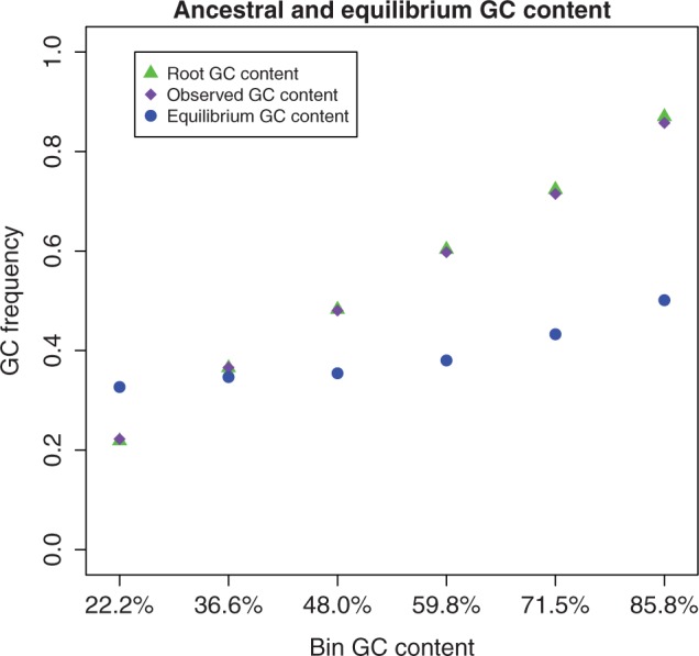
Variation in equilibrium and ancestral GC content with base composition. Exon alignments were binned in 6 classes according to GC content. On Y axis, we show great apes root (yellow), observed (purple), and equilibrium (blue) GC content in each bin (on X axis are bins ordered by increasing GC content) using CpG-PoMo10.

Variation within Exons

Finally, we addressed the issue of variation in evolutionary patterns between exonic positions. Different regions within an exon can vary in substitutional and compositional trends. 5′- and 3′-ends of nonterminal exons are GC-poorer than exon centers, and have stronger codon usage bias (Willie and Majewski 2004). This has been interpreted as the effect of selection on splicing motifs (reviewed in Chamary et al. 2006). In agreement with this hypothesis, codon usage bias in exon boundaries fits splicing motifs more than in exon centers (although not for every amino acid, Parmley and Hurst 2007). We analyzed variation in mutation and fixation biases within exons. We excluded terminal exons and divided sites in 3 bins. The 5′-bin contained the first 5 synonymous sites in each exon; the 3′-bin contained the last 5 sites; the central bin contained all the remaining sites. On each bin, we then estimated mutation rates and fixation biases as before.

We observe a higher GC content in exon centers, but extremely similar equilibrium frequencies in all bins (fig. 6A). Mutation rates do not vary noticeably (supplementary fig. S9B, Supplementary Material online). However, there are differences in fixation biases, with boundary sites showing preference for A over T, and the opposite pattern in exon centers (fig. 6B). Models that allow for these differences are preferable according to AIC, but not BIC (table 4; supplementary table S3, Supplementary Material online). Nevertheless, estimated differences are larger than expected just by error according to simulations (cf. supplementary figs. S9C and D, Supplementary Material online).

Fig. 6.

Variation within exons. Synonymous sites were binned according to their position within exons. The first and the last exon of each gene were excluded. The first 5 synonymous sites in each exon were assigned to the 5′-bin, the last 5 to the 3′-bin, the remaining to the central bin. On the X axis is the bin considered, on the Y axis are shown, respectively: (A) root, present, and equilibrium GC content, estimated with PoMo10; (B) fixation biases estimated with asy-CpG-PoMo10b. In 5′- and 3′-bins the number of sites is , in the other two . Error bars show the profile likelihood 95% confidence intervals.

Table 4.

Modeling Variation within Exons.

Model	Number of Parameters	AIC Score	BIC Score
Nulla	39	—	—
Mutb	57	−12.39	212.31
Selc	42	0.56	38.01
Mut-Seld	60	−20.54	241.62
Sel (G = C)e	40	−4.69	7.80
Mut-Sel (G = C)f	58	−12.58	224.60

Note.—Comparison of models for variation in evolutionary patterns between exon center and exon boundaries. A boundary bin includes 5 sites from 5′- and 3′-ends of each exon. A second center bin includes all the remaining sites. Model parameters were estimated on both boundary and center bins jointly.

^aasy-CpG-PoMo10b with no difference between bins.

^bDifferent mutation rates for the two bins.

^cDifferent selection coefficients .

^dBoth different mutation rates and fitness coefficients .

^eDifferent s_GC vs. s_AT fitness.

^fDifferent mutation rates and s_GC vs. s_AT fitness. We show AIC and BIC differences with respect to the Null model. The best BIC and AIC scores are underlined.

Discussion

Understanding intensity and variation of mutation and fixation biases is fundamental for the interpretation of evolutionary patterns. With our new model, PoMo, and with genome-scale data of within and between-species diversity, we disentangled and estimated mutational and fixation biases at synonymous sites of great apes.

Our estimates of mutation rates considerably differ from those of Lynch (2010), the only previous study, to our knowledge, that inferred relative mutation rates in humans while accounting for fixation biases (fig. 3A). Part of the difference might be due to the timescale considered (recent mutations in Lynch 2010, polymorphism and divergence here), and to the fact that we also include data from other great apes. However, we think that most of the discrepancy derives from transversions being over-represented in the missense and nonsense mutations (Gilis et al. 2001; De Maio et al. 2013) considered by (Lynch 2010; supplementary information and supplementary fig. S1, Supplementary Material online). Our analysis shows that estimates of relative mutation rates using phylogenetic data, as in Duret and Arndt (2008), are preferable, but for further comparative studies we suggest to use estimates from models accounting for fixation biases such as PoMo.

The strongest fixation bias that we detected favors GC over AT. In mammals, this phenomenon is generally attributed to gBGC. We inferred slightly lower estimates of gBGC than previous studies. Spencer et al. (2006) estimated the intensity of gBGC in the human genome from the allele frequency spectrum, while Lynch (2010) contrasted mutational patterns with nucleotide frequencies. The first approach considers the recent evolutionary past, while the second is informative of the fixation bias in the long term, probably on the scale of hundreds of millions of years (Duret et al. 2002). Our approach is intermediate, as it considers polymorphisms and divergence, but not base composition. Lynch (2010) estimated a gBGC intensity of , which was within the range 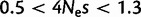from Spencer et al. (2006). We estimate to be . Although these values are not necessarily comparable, we recognized some additional causes for the small discrepancy. First, our method tends to slightly underestimate gBGC (fig. 2; supplementary fig. S12, Supplementary Material online). Second, we studied human–chimpanzee–orangutan data, and not only human. We observed a lower intensity of gBGC on the orangutan lineage ( vs. of the human–chimp lineage; table 2). A lower fixation bias in favor of GC nucleotides causes a shift in substitution rates towards AT, and therefore a reduction in GC*. A reduction in GC* in orangutan was previously observed by Polak et al. (2010). We suggest that the most likely explanation for reduced gBGC fixation bias in orangutan is a difference in historical effective population size (N_e), and not in the molecular repair bias itself (s). This is consistent with studies suggesting that N_e in orangutan was smaller than on human–chimp lineage: for the human–chimp ancestor and for the human–chimp–gorilla ancestor (Hobolth et al. 2007), in contrast to for the Bornean and Sumatran orangutan ancestor (Mailund et al. 2011).

Furthermore, we investigated variation of mutation and fixation biases along the exome with respect to present GC content. Regional variation in GC content is one of the most fascinating aspects of mammalian genomes, but its causes and consequences are still not well understood. Although some authors suggested that selection is the cause of GC content variation origin and maintenance (Bernardi 2000), most studies proposed neutral explanations, such as variation in mutation rates (Fryxell and Zuckerkandl 2000; Fryxell and Moon 2005) or gBGC (Duret and Galtier 2009). Here, we jointly estimated variation in mutation and fixation biases, therefore accounting for possible confounding effects of one on the other. We conclude that mutation rates (and in particular CpG hypermutability) and gBGC vary with base composition (fig. 4). Nevertheless, GC content decreases, and over time becomes more homogeneous across the genome (fig. 5), as concluded by previous studies as well (Duret et al. 2002, 2006; Meunier and Duret 2004). One of the possible explanations for the homogenization of GC content are changes in the recombination map, and therefore in gBGC intensity (Auton et al. 2012). Otherwise, a reduction in effective population size may have led to a decrease in the intensity and variation of gBGC effects. Additional studies on different mammalian clades are necessary to determine the most likely scenarios.

Finally, we measured differences in evolutionary patterns between exon centers and boundaries. Previous studies of base composition suggested that synonymous sites in different exonic positions are subject to different selective pressures due to splicing motifs (reviewed in Chamary et al. 2006). We confirmed these trends; in fact, we measured a fixation bias favoring A over T in boundaries of nonterminal exons, and T over A in exon centers (fig. 6B). This observation cannot be explained with gBGC, and is consistent with expectations of the hypothesis of selection on exonic splicing enhancers, since those are A-rich and T-poor (Parmley and Hurst 2007). However, our findings are only marginally significant, and they might be improved by including more individuals from more species in the future.

In conclusion, we presented a new phylogenetic model, PoMo, that can infer mutation and fixation biases from patterns of polymorphisms and divergence in populations/species related by any arbitrary history. We provide the software to replicate our analyses that assumes a sample of 10 sequences per species. This is a limitation of our implementation, and not of the model. In fact, the number of haplotypes considered from each population as well as the number of sites do not represent a considerable computational burden for our methods. Furthermore, as PoMo10 has fewer states than a codon model, it can be applied to phylogenies spanning several dozens of taxa (Seo and Kishino 2009; Gil et al. 2013).

PoMo can also be applied to the estimation of phylogenetic trees from population data. In fact, it has the potential to improve the resolution of short branches (relative to N_e), where classical methods for phylogenetic inference often fail due to incomplete lineage sorting and shared ancestral polymorphisms. These issues can already be accounted for by either making strong assumptions regarding recombination events (independent loci and no recombination within loci, see e.g., Heled and Drummond 2010) or by computationally demanding hidden Markov model approaches (Mailund et al. 2011). But, unlike PoMo, neither method is applicable to large numbers of individuals within-species, due to many possible coalescent trees.

Until now there are only few clades with genome-wide population data available from multiple species, such as primates and model organisms. This number is expected to grow in the near future, providing great opportunities to understand changes in evolutionary patterns.

Materials and Methods

Polymorphism-Aware Phylogenetic Models

Model Background

Phylogenetic substitution models represent DNA evolution as a continuous-time Markov process along a phylogenetic tree τ (for a review see Whelan et al. 2001). Different sites are generally assumed to evolve independently. Each point of τ represents a taxon at an instant, and tree bifurcations correspond to speciation events. Another common assumption is homogeneity: the evolutionary process does not change through time and among species. Nucleotide substitution models associate the points of τ to elements of the state space with certain probabilities. If a point of τ is in state C, it means that the corresponding taxon, at the corresponding time, had nucleotide C at the considered site of the genome. The phylogeny tips correspond to present, observable states.

States assigned to taxa can change in time, and the continuous-time Markov process modeling these changes is defined by an instantaneous rate matrix Q. Each entry Q_IJ of Q, with , is the rate at which nucleotide I is replaced by nucleotide J. Given Q, for any branch b of length t in τ it is possible to calculate the transition probability matrix . Entry of is the probability that the end of branch b is in state J, conditioned on the start being in state I. Matrix P(t) is used to calculate the likelihood of any parameter values θ via the Felsenstein pruning algorithm (Felsenstein 1981). The likelihood is the conditional probability of the data D given θ. Data D consist of DNA sequence alignments. Parameter estimates can be obtained by ML, that is, by determining the parameter values θ that maximize the likelihood function.

State Space

Our new models are similar in most aspects to standard phylogenetic nucleotide substitution models described earlier. The most important difference is that we expand the state space. We do not only include four states associated to nucleotides, but also further states representing polymorphisms. Nucleotide states in the new models represent sites with a fixed allele. Assuming at most two alleles per site per time per taxon, there exist six types of polymorphisms determined by the alleles simultaneously present in a taxon: , and . We define PoMo N (POlymorphism-aware MOdel with virtual population size N) as a phylogenetic model with N – 1 polymorphic states for each type of polymorphism. PoMo N state space has therefore elements, which means that any taxon at any considered time point can be assigned to any of the states. The N – 1 states associated to the same polymorphism type represent different allele frequencies within a virtual population of N haploid individuals. For example, polymorphic state i () of type represents a frequency of i/N for allele A and for allele C in a virtual population of N + 1 haploid individuals.

Definition of Instantaneous Rates

It is a common practice in population genetics to approximate the dynamics of a large real population with those of a small virtual population (Keightley and Eyre-Walker 2007; Kaiser and Charlesworth 2009; Zeng and Charlesworth 2009). To our knowledge, we present the first application of this approach to phylogenetics. We assume that the real population has effective population size , mutation rate per generation from allele I to J, fitness parameter for allele I, and number of generations . We define our virtual population as evolving according to a Moran model (Moran 1958) with population size N, mutation rate per generation from allele I to J, fitness parameter s_I for allele I, and number of generations t. The dynamics of a virtual population with properly scaled mutation rate () and selection coefficient (), are a good approximation of the real population, if time is scaled by the population size in both cases (t/N for the virtual population and for the real one) and if N is sufficiently large (Zeng and Charlesworth 2009, observed that even with N as small as 10 reasonable results could be achieved).

We make the assumption that the scaled mutation rate () is low, and allow mutations only at monomorphic sites in our virtual population (Vogl and Clemente 2012). Therefore, while our model is four-allelic, only two alleles can be present simultaneously in one population at a site. We represent the polymorphic state with i virtual individuals carrying allele I, and N – i carrying allele J, as .

The probability that the virtual population in a polymorphic state evolves to the state 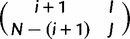in a single virtual generation is

(1)

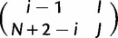Similarly, the probability to evolve from to is

(2)

The probability with which a new allele is introduced in the virtual population, that is, of evolving from monomorphic state I to polymorphic state 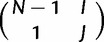in one virtual generation is

(3)

Within a single generation no other changes are allowed, in fact, virtual allele counts can only increase or decrease by one per generation. We call M_N the matrix of probabilities of allele frequency changes for one generation. Matrix M_N has dimension equal to the number of states, .

The last step in defining our model is transforming the Markov chain from discrete-time (in number of generations) into continuous-time. A continuous-time Markov chain is defined by its instantaneous rate matrix Q. We set the instantaneous rate matrix of our continuous-time process as 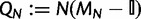, where is the identity matrix. Then, the probabilities of state changes in coalescent time t/N will be given by , where t as before represents the number of virtual generations, but can now take noninteger values. We list the entries of the rate matrix Q_N in supplementary table S9, Supplementary Material online.

After fitting the matrix Q_N to real data by ML, we estimated the scaled fitness parameters in the real population () as . The four fitness parameters (, and s_T) are defined up to an additive constant, and therefore correspond to three free parameters. When only gBGC is expected to drive fixation biases, we set and , reducing the number of free parameters describing fitness differences to one. Likewise, we estimated the scaled mutation rates () as .

Root Frequencies

Stationarity and reversibility are common and mathematically convenient assumptions for phylogenetic models, but are often not realistic (Galtier and Gouy 1995; Yang and Roberts 1995; Akashi et al. 2006; Gu and Li 2006). Here, we do not assume them. Because of nonstationarity of our model, state frequencies might change along τ, and root state frequencies π might differ from the observed frequencies. To define the entries of π, we use three additional free parameters (, and , where ) representing relative frequencies of fixed nucleotides at the root.

The root frequency of the polymorphic state with i virtual individuals carrying allele I, and N – i carrying allele J is:

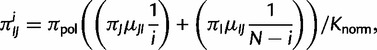(4)

where K_norm is a normalization factor, so that all root frequencies of polymorphic states sum up to . Under neutrality and rare mutations, the expected proportion of polymorphic sites with derived allele count i in a sample of N individuals is proportional to 1/i (e.g., see eq. 4.20 in Wakeley 2009). A root polymorphism can be derived from both alleles present in the population, we therefore take into account both possibilities in equation (4). The proportion of polymorphic states at the root, , is not a free parameter, but is set equal to the observed proportion of polymorphic states. In fact, could not be reliably estimated via ML, and its value did not affect the estimation of other parameters noticeably (supplementary information and table S1, Supplementary Material online). The root frequency of a fixed state I is .

PoMo10

All results in this study are based on PoMo10 (PoMo N with N = 10). PoMo10 has 58 states: 4 fixed states and 54 polymorphic states. In fact, for each of the 6 pairs of alleles (, and ), there are 9 polymorphic states for the possible allele counts (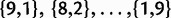). Therefore, PoMo10 has lower computational cost than a standard codon model (61 states), allowing genome-wide analysis of phylogenies with considerable numbers of species. PoMo10 approximates real population dynamics with those of a virtual population of 10 individuals. Although this is a rough approximation, it is expected to be sufficient for parameter estimation (Zeng and Charlesworth 2009, also confirmed by our simulations results). Smaller values of N generally resulted in considerable biases (supplementary fig. S16, Supplementary Material online).

For each species and site considered, we randomly extracted a sample of haploid size 10 (see Description of Data), and trivially associated the observed allele frequencies to the corresponding virtual frequency state, ignoring sampling variance. A limitation of PoMo10 is that it requires 10 sampled sequences for each species. A larger N is expected to result in improved estimates, but at computational costs (table 1).

PoMo10 Extensions: CpG Hypermutability and Strand-Asymmetry

When we assume no context-dependency or strand-asymmetry, we define six free parameters to describe mutation biases, one for each unordered pair of nucleotides (, etc.). Yet, mutation rates in mammals show strong dependency on the neighboring bases (Hwang and Green 2004). We extended PoMo10 to include the strongest context dependency, the hypermutability of CpG (nucleotide C followed by G) toward TpG or CpA. This is accounted for by an extra parameter that describes the mutation rate from C to T and from G to A in a CpG context. We call this model CpG-PoMo10 (for detailed description of rates see supplementary information, Supplementary Material online). To estimate parameters of CpG-PoMo10, we only used synonymous sites whose preceding and following bases are constant among the considered species. We generally have three free parameters describing nucleotide frequencies at the root, but with context dependency this number increases to 12 to account for different frequencies in different CpG contexts.

We further extended CpG-PoMo10 to account for hypermutability of transversions in CpG context (from CpG to ApG, GpG, CpC, and CpT). The resulting model, CpG-PoMo10b, has two additional free mutational parameters (for details see supplementary information, Supplementary Material online).

Finally, we accounted for strand-specificity of mutation rates (Hwang and Green 2004; Polak and Arndt 2008). In the resulting model, asy-CpG-PoMo10b, the constraints for strand-symmetry (e.g., ) are relaxed, and therefore 9 extra free mutational parameters are necessary with respect to CpG-PoMo10b, for a total of 18 (for details see supplementary information, Supplementary Material online).

Model Implementation

In this study, we assume that the tree topology is known and fixed (supplementary fig. S17, Supplementary Material online), and we estimate all branch lengths in the 4-species rooted tree. Lists of number of free parameters for different models are included in tables 2–4.

Parameter estimation was performed via ML with the conjugate gradient algorithm implemented in HyPhy (Pond et al. 2005). For this purpose, we produced custom scripts in HyPhy Batch Language (supplementary file S1 [Supplementary Material online] describes asy-CpG-PoMo10b and PoMo10 for the case and ). We always estimated all free parameters simultaneously. The scripts that we provide require 10 sequences sampled from each species. This is a limitation of the present state of our software, but not of the model (table 1 and discussion). We used different starting points for the conjugate gradient iterations on the whole real data set, and observed consistency of different optimization runs (supplementary information and supplementary fig. S2, Supplementary Material online).

Description of Data

Great Apes Data Set

We constructed an exome-wide, inter- and intraspecies data set of alignments of 4-fold degenerate (synonymous) sites from H. sapiens, P. troglodytes, Pon. abelii, and Pon. pygmaeus (respectively human, chimpanzee, and Sumatran and Bornean orangutan).

First, CCDS (Pruitt et al. 2009) alignments of H. sapiens, P. troglodytes, and Pon. abelii (references hg18, panTro2, and ponAbe2) were downloaded from the UCSC genome browser (http://genome.ucsc.edu, last accessed August 8, 2013). Only CCDS alignments satisfying the following requirements were retained for the subsequent analyses: divergence from human reference below 10%, no gene duplication in any species, start and stop codons conserved, no frame-shifting gaps, no gap longer than 30 bases, no nonsense codon, no gene shorter than 21 bases, no gene with different number of exons in different species, or genes in different chromosomes in different species (chromosomes 2a and 2b in nonhumans were identified with human chromosome 2). From the remaining CCDSs (9,695 genes and 79,677 exons), we extracted synonymous sites. We only considered third codon positions where the first two nucleotides of the same codon were conserved in the alignment, as well as the first position of the next codon.

Then, population data were added to the species alignments. Human single nucleotide polymorphisms (SNPs) from 59 Yoruban (Nigerian) individuals (haploid sample size ) sequenced from the 1,000 genomes pilot project (1000 Genomes Project Consortium 2010) were downloaded (ftp://ftp.1000genomes.ebi.ac.uk/vol1/ftp/, last accessed August 8, 2013) and included the alignments. Similarly, we added SNP data of 10 western chimpanzee individuals (haploid sample size ) sequenced by the PanMap project (Auton et al. 2012) and downloaded from ftp://birch.well.ox.ac.uk/haplotypes/ (last accessed August 8, 2013). Orangutan SNP data for the two species considered, each with five sequenced individuals (haploid sample size ≤ 10, Locke et al. 2011), were kindly provided to us by X. Ma (in preparation) and are now available online (http://www.ncbi.nlm.nih.gov/projects/SNP/snp_viewTable.cgi?type=contact&handle=WUGSC_SNP&batch_id=1054968, last accessed August 8, 2013). We sub-sampled 10 alleles without replacement for each species and site. The final total number of synonymous sites included was 1,950,006 (for more details on real data sets see supplementary tables S4–S6, Supplementary Material online).

The collection of all synonymous site alignments in the great apes data set in valid format for PoMo10 is provided as supplementary file S2, Supplementary Material online. Custom scripts to convert SNP data from VCF v4.0 format into PoMo10 states, and to convert multi-species alignments into HyPhy input files, are also provided as supplementary file S3, Supplementary Material online.

Simulations

We simulated a population of 50 diploid individuals evolving according to a phylogenetic tree (supplementary fig. S17, Supplementary Material online), where a branch bifurcation represents the duplication and split of a population. Evolution was simulated according to a Wright–Fisher model with sexual reproduction using simuPOP (Peng and Kimmel 2005) and custom Python scripts. Phylogeny and mutation rates were set so to have similar divergence and diversity levels to those in real data (supplementary table S4, Supplementary Material online).

First, we simulated five scenarios, in which we progressively added demographic events. The first scenario consisted of a constant-size population phylogeny. In the second scenario, we added a bottleneck on the human branch. In the third, we made a population expansion follow the bottleneck. In the fourth, we further added migration between the two orangutan species. Finally, we reduced population size in the second half of the chimpanzee branch (for further details about simulated demographic events see supplementary information, Supplementary Material online).

In a second set of simulations, we included CpG context. We used root frequencies and mutation rates as estimated from GC-rich and GC-poor bins (the extreme bins in figs. 4 and 5; for a detailed description of mutational parameters in simulations, see supplementary information, Supplementary Material online). For both the GC contents considered, we simulated three selective regimes with a GC versus AT fitness difference of 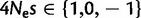, for a total of six scenarios. For each scenario, we simulated 10⁶ independent sites, and then sub-sampled data sets of varying sizes (ranging from 10⁴ to sites), with 10 replicates for each size.

Supplementary Material

Supplementary files S1–S3, figures S1–S18, and tables S1–S9 are available at Molecular Biology and Evolution online (http://http://mbe.oxfordjournals.org/).

References

- 1000 Genomes Project Consortium. A map of human genome variation from population-scale sequencing. Nature. 2010;467:1061–1073. doi: 10.1038/nature09534. [DOI] [PMC free article] [PubMed] [Google Scholar]
- Akashi H, Ko W, Piao S, John A, Goel P, Lin C, Vitins A. Molecular evolution in the Drosophila melanogaster species subgroup: frequent parameter fluctuations on the timescale of molecular divergence. Genetics. 2006;172:1711–1726. doi: 10.1534/genetics.105.049676. [DOI] [PMC free article] [PubMed] [Google Scholar]
- Alvarez-Valin F, Clay O, Cruveiller S, Bernardi G. Inaccurate reconstruction of ancestral GC levels creates a vanishing isochores effect. Mol Phylogenet Evol. 2004;31:788–793. doi: 10.1016/j.ympev.2004.01.016. [DOI] [PubMed] [Google Scholar]
- Auton A, Fledel-Alon A, Pfeifer S, et al. (23 co-authors) A fine-scale chimpanzee genetic map from population sequencing. Science. 2012;336:193–198. doi: 10.1126/science.1216872. [DOI] [PMC free article] [PubMed] [Google Scholar]
- Belle E, Duret L, Galtier N, Eyre-Walker A. The decline of isochores in mammals: an assessment of the GC content variation along the mammalian phylogeny. J Mol Evol. 2004;58:653–660. doi: 10.1007/s00239-004-2587-x. [DOI] [PubMed] [Google Scholar]
- Bernardi G. Isochores and the evolutionary genomics of vertebrates. Gene. 2000;241:3–17. doi: 10.1016/s0378-1119(99)00485-0. [DOI] [PubMed] [Google Scholar]
- Bryant D, Bouckaert R, Felsenstein J, Rosenberg NA, RoyChoudhury A. Inferring species trees directly from biallelic genetic markers: bypassing gene trees in a full coalescent analysis. Mol Biol Evol. 2012;29:1917–1932. doi: 10.1093/molbev/mss086. [DOI] [PMC free article] [PubMed] [Google Scholar]
- Chamary J, Parmley J, Hurst L. Hearing silence: non-neutral evolution at synonymous sites in mammals. Nat Rev Genet. 2006;7:98–108. doi: 10.1038/nrg1770. [DOI] [PubMed] [Google Scholar]
- Charlesworth B, Bartolomé C, Noël V. The detection of shared and ancestral polymorphisms. Genet Res. 2005;86:149–157. doi: 10.1017/S0016672305007743. [DOI] [PubMed] [Google Scholar]
- Clark A. Neutral behavior of shared polymorphism. Proc Natl Acad Sci U S A. 1997;94:7730. doi: 10.1073/pnas.94.15.7730. [DOI] [PMC free article] [PubMed] [Google Scholar]
- Clay O, Caccio S, Zoubak S, Mouchiroud D, Bernardi G. Human coding and noncoding DNA: compositional correlations. Mol Phylogenet Evol. 1996;5:2–12. doi: 10.1006/mpev.1996.0002. [DOI] [PubMed] [Google Scholar]
- De Maio N, Holmes I, Schlötterer C, Kosiol C. Estimating empirical codon hidden markov models. Mol Biol Evol. 2013;30:725–736. doi: 10.1093/molbev/mss266. [DOI] [PMC free article] [PubMed] [Google Scholar]
- Duret L. Mutation patterns in the human genome: more variable than expected. PLoS Biol. 2009;7:e1000028. doi: 10.1371/journal.pbio.1000028. [DOI] [PMC free article] [PubMed] [Google Scholar]
- Duret L, Arndt P. The impact of recombination on nucleotide substitutions in the human genome. PLoS Genet. 2008;4:e1000071. doi: 10.1371/journal.pgen.1000071. [DOI] [PMC free article] [PubMed] [Google Scholar]
- Duret L, Eyre-Walker A, Galtier N. A new perspective on isochore evolution. Gene. 2006;385:71–74. doi: 10.1016/j.gene.2006.04.030. [DOI] [PubMed] [Google Scholar]
- Duret L, Galtier N. Biased gene conversion and the evolution of mammalian genomic landscapes. Annu Rev Genom Hum Genet. 2009;10:285–311. doi: 10.1146/annurev-genom-082908-150001. [DOI] [PubMed] [Google Scholar]
- Duret L, Hurst L. The elevated GC content at exonic third sites is not evidence against neutralist models of isochore evolution. Mol Biol Evol. 2001;18:757–762. doi: 10.1093/oxfordjournals.molbev.a003858. [DOI] [PubMed] [Google Scholar]
- Duret L, Semon M, Piganeau G, Mouchiroud D, Galtier N. Vanishing GC-rich isochores in mammalian genomes. Genetics. 2002;162:1837–1847. doi: 10.1093/genetics/162.4.1837. [DOI] [PMC free article] [PubMed] [Google Scholar]
- Dutheil J, Ganapathy G, Hobolth A, Mailund T, Uyenoyama M, Schierup M. Ancestral population genomics: the coalescent hidden Markov model approach. Genetics. 2009;183:259–274. doi: 10.1534/genetics.109.103010. [DOI] [PMC free article] [PubMed] [Google Scholar]
- Eyre-Walker A, Hurst L. The evolution of isochores. Nat Rev Genet. 2001;2:549–555. doi: 10.1038/35080577. [DOI] [PubMed] [Google Scholar]
- Eyre-Walker A, Keightley P. The distribution of fitness effects of new mutations. Nat Rev Genet. 2007;8:610–618. doi: 10.1038/nrg2146. [DOI] [PubMed] [Google Scholar]
- Felsenstein J. Evolutionary trees from DNA sequences: a maximum likelihood approach. J Mol Evol. 1981;17:368–376. doi: 10.1007/BF01734359. [DOI] [PubMed] [Google Scholar]
- Fryxell K, Moon W. CpG mutation rates in the human genome are highly dependent on local GC content. Mol Biol Evol. 2005;22:650–658. doi: 10.1093/molbev/msi043. [DOI] [PubMed] [Google Scholar]
- Fryxell K, Zuckerkandl E. Cytosine deamination plays a primary role in the evolution of mammalian isochores. Mol Biol Evol. 2000;17:1371–1383. doi: 10.1093/oxfordjournals.molbev.a026420. [DOI] [PubMed] [Google Scholar]
- Galtier N, Duret L, Glémin S, Ranwez V. GC-biased gene conversion promotes the fixation of deleterious amino acid changes in primates. Trends Genet. 2009;25:1–5. doi: 10.1016/j.tig.2008.10.011. [DOI] [PubMed] [Google Scholar]
- Galtier N, Gouy M. Inferring phylogenies from DNA sequences of unequal base compositions. Proc Natl Acad Sci U S A. 1995;92:11317–11321. doi: 10.1073/pnas.92.24.11317. [DOI] [PMC free article] [PubMed] [Google Scholar]
- Gil M, Zanetti MS, Zoller S, Anisimova M. CodonPhyML: fast maximum likelihood phylogeny estimation under codon substitution models. Mol Biol Evol. 2013;30:1270–1280. doi: 10.1093/molbev/mst034. [DOI] [PMC free article] [PubMed] [Google Scholar]
- Gilis D, Massar S, Cerf N, Rooman M. Optimality of the genetic code with respect to protein stability and amino-acid frequencies. Genome Biol. 2001;2 doi: 10.1186/gb-2001-2-11-research0049. RESEARCH0049. [DOI] [PMC free article] [PubMed] [Google Scholar]
- Gronau I, Arbiza L, Mohammed J, Siepel A. Inference of natural selection from interspersed genomic elements based on polymorphism and divergence. Mol Biol Evol. 2013;30:1159–1171. doi: 10.1093/molbev/mst019. [DOI] [PMC free article] [PubMed] [Google Scholar]
- Gu J, Li W. Are GC-rich isochores vanishing in mammals? Gene. 2006;385:50–56. doi: 10.1016/j.gene.2006.03.026. [DOI] [PubMed] [Google Scholar]
- Haddrill P, Thornton K, Charlesworth B, Andolfatto P. Multilocus patterns of nucleotide variability and the demographic and selection history of Drosophila melanogaster populations. Genome Res. 2005;15:790–799. doi: 10.1101/gr.3541005. [DOI] [PMC free article] [PubMed] [Google Scholar]
- Heled J, Drummond A. Bayesian inference of species trees from multilocus data. Mol Biol Evol. 2010;27:570–580. doi: 10.1093/molbev/msp274. [DOI] [PMC free article] [PubMed] [Google Scholar]
- Hernandez R, Williamson S, Zhu L, Bustamante C. Context-dependent mutation rates may cause spurious signatures of a fixation bias favoring higher GC-content in humans. Mol Biol Evol. 2007;24:2196–2202. doi: 10.1093/molbev/msm149. [DOI] [PubMed] [Google Scholar]
- Hobolth A, Christensen O, Mailund T, Schierup M. Genomic relationships and speciation times of human, chimpanzee, and gorilla inferred from a coalescent hidden Markov model. PLoS Genet. 2007;3:e7. doi: 10.1371/journal.pgen.0030007. [DOI] [PMC free article] [PubMed] [Google Scholar]
- Hodgkinson A, Eyre-Walker A. Variation in the mutation rate across mammalian genomes. Nat Rev Genet. 2011;12:756–766. doi: 10.1038/nrg3098. [DOI] [PubMed] [Google Scholar]
- Hodgkinson A, Ladoukakis E, Eyre-Walker A. Cryptic variation in the human mutation rate. PLoS Biol. 2009;7:e1000027. doi: 10.1371/journal.pbio.1000027. [DOI] [PMC free article] [PubMed] [Google Scholar]
- Hwang D, Green P. Bayesian Markov chain Monte Carlo sequence analysis reveals varying neutral substitution patterns in mammalian evolution. Proc Natl Acad Sci U S A. 2004;101:13994–14001. doi: 10.1073/pnas.0404142101. [DOI] [PMC free article] [PubMed] [Google Scholar]
- Kaiser VB, Charlesworth B. The effects of deleterious mutations on evolution in non-recombining genomes. Trends Genet. 2009;25:9–12. doi: 10.1016/j.tig.2008.10.009. [DOI] [PubMed] [Google Scholar]
- Keightley PD, Eyre-Walker A. Joint inference of the distribution of fitness effects of deleterious mutations and population demography based on nucleotide polymorphism frequencies. Genetics. 2007;177:2251–2261. doi: 10.1534/genetics.107.080663. [DOI] [PMC free article] [PubMed] [Google Scholar]
- Liu L. BEST: Bayesian estimation of species trees under the coalescent model. Bioinformatics. 2008;24:2542–2543. doi: 10.1093/bioinformatics/btn484. [DOI] [PubMed] [Google Scholar]
- Locke DP, Hillier LW, Warren WC, et al. (101 co-authors) Comparative and demographic analysis of orangutan genomes. Nature. 2011;469:529–533. doi: 10.1038/nature09687. [DOI] [PMC free article] [PubMed] [Google Scholar]
- Lynch M. Rate, molecular spectrum, and consequences of human mutation. Proc Natl Acad Sci U S A. 2010;107:961–968. doi: 10.1073/pnas.0912629107. [DOI] [PMC free article] [PubMed] [Google Scholar]
- Maddison W, Knowles L. Inferring phylogeny despite incomplete lineage sorting. Syst Biol. 2006;55:21–30. doi: 10.1080/10635150500354928. [DOI] [PubMed] [Google Scholar]
- Mailund T, Dutheil J, Hobolth A, Lunter G, Schierup M. Estimating divergence time and ancestral effective population size of Bornean and Sumatran orangutan subspecies using a coalescent hidden Markov model. PLoS Genet. 2011;7:e1001319. doi: 10.1371/journal.pgen.1001319. [DOI] [PMC free article] [PubMed] [Google Scholar]
- McDonald JH, Kreitman M. Adaptive protein evolution at the Adh locus in Drosophila. Nature. 1991;351:652–654. doi: 10.1038/351652a0. [DOI] [PubMed] [Google Scholar]
- Meunier J, Duret L. Recombination drives the evolution of GC-content in the human genome. Mol Biol Evol. 2004;21:984–990. doi: 10.1093/molbev/msh070. [DOI] [PubMed] [Google Scholar]
- Moran P. Random processes in genetics. Math Proc Cambridge Philos Soc. 1958;54:60–71. [Google Scholar]
- Nagylaki T. Evolution of a finite population under gene conversion. Proc Natl Acad Sci U S A. 1983;80:6278–6281. doi: 10.1073/pnas.80.20.6278. [DOI] [PMC free article] [PubMed] [Google Scholar]
- Parmley J, Hurst L. Exonic splicing regulatory elements skew synonymous codon usage near intron-exon boundaries in mammals. Mol Biol Evol. 2007;24:1600–1603. doi: 10.1093/molbev/msm104. [DOI] [PubMed] [Google Scholar]
- Peng B, Kimmel M. simuPOP: a forward-time population genetics simulation environment. Bioinformatics. 2005;21:3686–3687. doi: 10.1093/bioinformatics/bti584. [DOI] [PubMed] [Google Scholar]
- Polak P, Arndt P. Transcription induces strand-specific mutations at the 5 end of human genes. Genome Res. 2008;18:1216–1223. doi: 10.1101/gr.076570.108. [DOI] [PMC free article] [PubMed] [Google Scholar]
- Polak P, Querfurth R, Arndt P. The evolution of transcription-associated biases of mutations across vertebrates. BMC Evol Biol. 2010;10:187. doi: 10.1186/1471-2148-10-187. [DOI] [PMC free article] [PubMed] [Google Scholar]
- Pollard D, Iyer V, Moses A, Eisen M. Widespread discordance of gene trees with species tree in Drosophila: evidence for incomplete lineage sorting. PLoS Genet. 2006;2:e173. doi: 10.1371/journal.pgen.0020173. [DOI] [PMC free article] [PubMed] [Google Scholar]
- Pond SLK, Frost SDW, Muse SV. HyPhy: hypothesis testing using phylogenies. Bioinformatics. 2005;21:676–679. doi: 10.1093/bioinformatics/bti079. [DOI] [PubMed] [Google Scholar]
- Pruitt K, Harrow J, Harte R, et al. (49 co-authors) The consensus coding sequence (CCDS) project: identifying a common protein-coding gene set for the human and mouse genomes. Genome Res. 2009;19:1316–1323. doi: 10.1101/gr.080531.108. [DOI] [PMC free article] [PubMed] [Google Scholar]
- Ratnakumar A, Mousset S, Glémin S, Berglund J, Galtier N, Duret L, Webster M. Detecting positive selection within genomes: the problem of biased gene conversion. Philos Trans R Soc Lond B Biol Sci. 2010;365:2571–2580. doi: 10.1098/rstb.2010.0007. [DOI] [PMC free article] [PubMed] [Google Scholar]
- RoyChoudhury A, Felsenstein J, Thompson E. A two-stage pruning algorithm for likelihood computation for a population tree. Genetics. 2008;180:1095–1105. doi: 10.1534/genetics.107.085753. [DOI] [PMC free article] [PubMed] [Google Scholar]
- Schneider A, Charlesworth B, Eyre-Walker A, Keightley PD. A method for inferring the rate of occurrence and fitness effects of advantageous mutations. Genetics. 2011;189:1427–1437. doi: 10.1534/genetics.111.131730. [DOI] [PMC free article] [PubMed] [Google Scholar]
- Seo T, Kishino H. Statistical comparison of nucleotide, amino acid, and codon substitution models for evolutionary analysis of protein-coding sequences. Syst Biol. 2009;58:199. doi: 10.1093/sysbio/syp015. [DOI] [PubMed] [Google Scholar]
- Spencer C, Deloukas P, Hunt S, Mullikin J, Myers S, Silverman B, Donnelly P, Bentley D, McVean G. The influence of recombination on human genetic diversity. PLoS Genet. 2006;2:e148. doi: 10.1371/journal.pgen.0020148. [DOI] [PMC free article] [PubMed] [Google Scholar]
- Squartini F, Arndt P. Quantifying the stationarity and time reversibility of the nucleotide substitution process. Mol Biol Evol. 2008;25:2525–2535. doi: 10.1093/molbev/msn169. [DOI] [PubMed] [Google Scholar]
- Vogl C, Clemente F. The allele-frequency spectrum in a decoupled Moran model with mutation, drift, and directional selection, assuming small mutation rates. Theor Popul Biol. 2012;81:197–209. doi: 10.1016/j.tpb.2012.01.001. [DOI] [PMC free article] [PubMed] [Google Scholar]
- Wakeley J. Coalescent theory: an introduction. 2009 Greenwood Village: Roberts & Company Publishers. [Google Scholar]
- Whelan S, Liò P, Goldman N. Molecular phylogenetics: state-of-the-art methods for looking into the past. Trends Genet. 2001;17:262–272. doi: 10.1016/s0168-9525(01)02272-7. [DOI] [PubMed] [Google Scholar]
- Willie E, Majewski J. Evidence for codon bias selection at the pre-mRNA level in eukaryotes. Trends Genet. 2004;20:534–538. doi: 10.1016/j.tig.2004.08.014. [DOI] [PubMed] [Google Scholar]
- Wilson D, Hernandez R, Andolfatto P, Przeworski M. A population genetics-phylogenetics approach to inferring natural selection in coding sequences. PLoS Genet. 2011;7:e1002395. doi: 10.1371/journal.pgen.1002395. [DOI] [PMC free article] [PubMed] [Google Scholar]
- Yang Z, Nielsen R. Mutation-selection models of codon substitution and their use to estimate selective strengths on codon usage. Mol Biol Evol. 2008;25:568–579. doi: 10.1093/molbev/msm284. [DOI] [PubMed] [Google Scholar]
- Yang Z, Roberts D. On the use of nucleic acid sequences to infer early branchings in the tree of life. Mol Biol Evol. 1995;12:451–458. doi: 10.1093/oxfordjournals.molbev.a040220. [DOI] [PubMed] [Google Scholar]
- Zeng K, Charlesworth B. Estimating selection intensity on synonymous codon usage in a nonequilibrium population. Genetics. 2009;183:651–662. doi: 10.1534/genetics.109.101782. [DOI] [PMC free article] [PubMed] [Google Scholar]
Associated Data
This section collects any data citations, data availability statements, or supplementary materials included in this article.