Abstract
The long-standing interior problem has important mathematical and practical implications. The recently developed interior tomography methods have produced encouraging results. A particular scenario for theoretically exact interior reconstruction from truncated projections is that there is a known subregion in the region of interest (ROI). In this paper, we improve a novel continuous singular value decomposition (SVD) method for interior reconstruction assuming a known subregion. First, two sets of orthogonal eigen-functions are calculated for the Hilbert and image spaces respectively. Then, after the interior Hilbert data are calculated from projection data through the ROI, they are projected onto the eigen-functions in the Hilbert space, and an interior image is recovered by a linear combination of the eigen-functions with the resulting coefficients. Finally, the interior image is compensated for the ambiguity due to the null space utilizing the prior subregion knowledge. Experiments with simulated and real data demonstrate the advantages of our approach relative to the projection onto convex set type interior reconstructions.
Keywords: Hilbert transform, interior tomography, singular value decomposition (SVD), X-ray computed tomography (CT)
I. Introduction
AT THE present time, the computed tomography (CT) theory is undergoing rapid development. In many applications of CT such as biomedical imaging, industrial nondestructive testing, and security screening, situations are common in which a region of interest (ROI) is small and located strictly inside the object support (interior ROI). Clearly, the ROI-focused scanning and subsequent reconstruction may minimize radiation dose, handle large objects, shorten scanning time, and reduce engineering cost [1]. Over the past decades, many efforts were spent on developing local reconstruction algorithms which take only ROI data, but produce qualitative, rather than quantitative, images [2]-[6].
For a long time, due to the nonlocal property of the Radon transform inversion, it has been widely believed that theoretically exact local reconstruction cannot be done only from projection data through an ROI, and indeed a counter example was explicitly constructed showing the nonuniqueness of the solution to the interior problem [7]. Interestingly, this problem has been recently revisited with important theoretical and practical results [8]-[10]. In the differentiated back-projection (DBP) framework, the solution to the interior problem was proved to be unique if there is a known subregion inside a ROI [11]-[13]. A theoretical basis was laid down in early 1990s when Gelfand and Graev established a fundamental relationship between the Hilbert transform of an image along a line and differentiated projection data of the image [14], [15].
For interior reconstruction, there are several DBP methods available, most of which are based on the projection onto convex sets (POCS) (usually add one more constraint of L1 norm minimization to the image) [16], [17]. However, the iterative process is computationally expensive and can be prohibitively slow for real-world applications. As an alternative, an SVD-based DBP approach was proposed, which allows a noniterative interior reconstruction [18], [19]. The SVD approach is much faster than its iterative counterpart and produces encouraging preliminary results.
In this paper, we further develop the SVD approach for interior tomography. Based on the latest continuous SVD formulation setup by Katsevich [20], here we propose a new interior tomography algorithm. First, two sets of orthogonal eigen-functions are calculated for the Hilbert and image spaces respectively. Then, after the interior Hilbert data are calculated from truncated projections through the ROI, they are projected onto the eigen-functions in the Hilbert space, and an interior image is recovered by a linear combination of the eigen-functions in the image space with the resulting coefficients. Finally, the quality of interior reconstruction is improved using a compensation method which utilizes prior subregion knowledge. Numerical and clinical experiments are performed to show the advantages of our approach relative to the POCS iterative reconstruction algorithms.
The rest of this paper is organized as follows. In the next section, the basic facts about the truncated Hilbert transform (THT) and its SVD are summarized. In the third section, the SVD method is introduced for the ROI-focused reconstruction, which utilizes a continuous SVD theory and a null-space compensation technique. In the fourth section, numerical and pre-clinical experimental results are presented. Finally, relevant issues are discussed and the paper is concluded in the last section.
II. SVD-THT Theory
Very recently, Katsevich developed an analytical SVD method for the truncated Hilbert transform (THT). It can be directly used to solve the interior problem from the DBP data. The major results can be summarized as follows.
For any two real numbers ai, aj ∈ R, and any ω(y) ∈ C∞([ai, aj]), define a transform Hij: L2([ai, aj]) → L2(R) that
| (1) |
Also, for any four real numbers, a1 < a2 < a3 < a4, define a differential operator L
| (2) |
where ω ∈ C∞(R) and
| (3) |
and dx represents a derivative operator with respect to x. Then a Sturm–Liouville boundary value problem can be described as
| (4) |
This is a singular Sturm–Liouville problem with limit-circle nonoscillatory end-points [19]. It is known that its eigenvalues satisfy
| (5) |
and the associated normalized eigen-functions {φn(y), a2 < y < a3}, n ≥ 0, are orthogonal and complete in L2([a2, a3]). From (1) and (2) it can be deduced that for any φ(y), which is sufficiently smooth
| (6) |
Define ψn (x) ∈ L2([a1, a4]) in terms of φn as
| (7) |
where ∥·∥14 is the norm in L2([a1, a4]). By (4) and (6), we have
| (8) |
With (8), the orthonormality of the set {ψn, n ≥ 0} in L2([a1, a4]) can be proved [19]. Using the results in [21]
| (9) |
Thereby, given that
| (10) |
one has
| (11) |
Therefore, the set {φn, ψn, νn}, n ≥ 0 forms an SVD of the operator H23 : L2([a2, a3]) → L2([a1, a4]). Let ψ(x) and φ(y) denote functions compactly supported on ([a1, a4]) and ([a2, a3]), respectively. Suppose also ψ(x) and φ(y) satisfy
| (12) |
We can decompose φ(y) according to
| (13) |
and recover ψ(x by the formula
| (14) |
in the SVD sense (i.e., the difference between the true solution and the right side of (14) is a function from the null-space of the operator H14 : L2([a1, a4]) → L2([a2, a3]).
III. Image Reconstruction
A. DBP Reconstruction Theory
Let f(x, y) denote a 2-D compactly supported piecewise continuous function. The Radon transform of f(x, y) can be expressed as
| (15) |
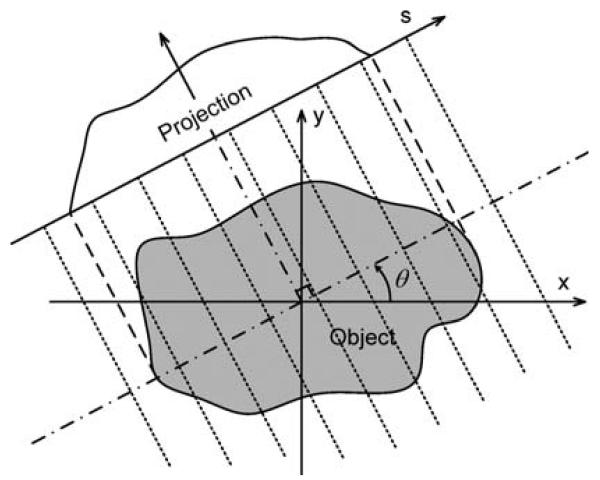
where θ is a projection angle, and s is the offset between an arbitrary X-ray path and the origin. The projection geometry is shown in Fig. 1. Let L(s, θ) denote the line defined by L(s, θ) = {x ∈ R2 : x · (cos θ, sin θ) = s}. Referring to the DBP reconstruction theory, the DBP data along L(s, θ) are calculated as [16]
| (16) |
To simplify notations, we introduce a 1-D coordinate t along L(s, θ). The function f(x, y) restricted to L(s, θ) is denoted as fL(t). In particular, if (x, y) ∈ L(s, θ), then
| (17) |
Similarly, the restriction of g(x, y) onto L is denoted gL(t). Assume that along L the object is supported on the interval a1 < t < a4. Then, the Hilbert transform of fL(t) equals gL(s, θ) [16]:
| (18) |
Equations (16) and (18) establish a relationship between the object function and its DBP data. Given, p(s, θ), one can compute the DBP data and invert the Hilbert transform along any line L in the field-of-view (FOV). In our paper, we call such a line a chord. This process gives us f(x, y) on different chords.
Fig. 1.
Illustration of projection geometry.
By (16), the calculation of DBP data requires that p(s, θ) covers at least a 180° range for any point on the chord L. In the case of interior reconstruction, p(s, θ) is truncated along s and only an interior ROI meets the data requirement. In other words, interior DBP data are truncated. In the following, we use the SVD-THT method to address the interior reconstruction.
B. Inversion of the Truncated Hilbert Transform
Let us choose a chord L through an ROI. We represent an object along this line as f(t), and its DBP data as g(t). Let t = a1, a4 denote the boundary of the object support, and let t = a2, a3 denote the boundary of the ROI. With the interior problem, we have a1 < a2 < a3 < a4, and the available DBP data g(t) are truncated. The available part of DBP is denoted by g23(t), t ∈ (a2, a3). According to the SVD-THT theory, fSVD(t) the estimation of f(t), can be done using the following steps:
Solve the Sturm–Liouville problem defined by (4). The result is a set of eigen-functions φn(t), n ≥ 0, which are orthonormal on (a2, a3). Then, apply (7) to obtain functions ψn(t), n ≥ 0, which are orthonormal on (a1, a4).
Compute the DBP data g23(t) using (16).
- Choose N and decompose g23(t) in terms of φn(t), 0 ≤ n ≤ N
(19) - Compute fSVD(t) by a linear combination of ψn(t), 0 ≤ n ≤ N, following (14) as
(20) An estimated solution of ROI along the line L is given by fSVD(t), a2 ≤ t ≤ a3.
C. Null Space Compensation
Theoretically speaking, truncated DBP data (ROI data) do not provide suf cient information for exact reconstruction of the ROI image. The missing data lead to a nontrivial null space associated with the truncated Hilbert transform (THT). To compensate for the nonuniqueness of SVD-THT reconstruction, a set of basis functions on the null space is used to estimate the missing information.
Suppose there are M basis functions in the null space. Denote each of them as fnull,m(t), m = 1, 2,…,M. The compensation can be performed by adding a linear combination of fnull,m(t) to fSVD(t). The compensated ROI can be expressed as
| (21) |
where km is the weighting factor for the mth null space base function. The values of km can be estimated using an optimization method which will be described in the following section.
Generation of fnull,m(t) can be done in various ways. As the DBP data are known inside the ROI, the only requirement for generating fnull,m(t) is that the Hilbert transform of fnull,m(t) be equal to zero on the ROI. In our work, this is done as follows. First, along the chord L select the regions which are inside the object support but outside the ROI. In our case these are the regions (a1, a2) and (a3, a4). Then divide them into M sub-segments seg1, seg2,…,segM without overlapping. To avoid singularities at the four boundary points the actual regions are chosen as (a1 + δ, a2 − δ) and (a3 + δ, a4 − δ) where δ > 0 is a small number. On each subsegment, a linear function gnull,m(t) in the DBP space is created
| (22) |
where bm is a number corresponding to the mth subsegment. When gnull,m(t) are generated in the range of the nite Hilbert transform (FHT), the original functions in the image space can be calculated by the following inverse nite Hilbert transform (iFHT) equation:
| (23) |
Here, is a weight function. Equation (23) is a special version of the iFHT that requires no line integral constant of fnull,m(t) [22]. As fnull,m(t) is unknown in our problem, using (23) avoids the calculation of the integral constant. The fact that gnull,m(t) is in the range of FHT implies that the Hilbert transform of fnull,m(t) on (a1, a4) is precisely gnull,m(t). It also guarantees that fnull,m(t) is in the null space, and the ROI region of the DBP data is not affected by the compensation. According to the reference, insuring that the range condition is satisfied requires [22]
| (24) |
The first equation in (24) can be ful lled by adjusting bm for each gnull,m(t). This derivation is trivial and is omitted. The second equation in (24) is satisfied automatically for functions of the type in (22).
D. Constrained Optimization
In this section, we develop an optimization method, which incorporates a known subregion as well as other forms of prior knowledge into the null space compensation.
First, a known subregion inside the ROI is considered. Assume that the known part of f(t) is represented in the form f(t) = fpri(t), t ∈ [a5, a6] where [a5, a6] is a subinterval inside the ROI. Then, the optimization problem can be described as
| (25) |
The second form of prior knowledge is based on the following observation. Inside the ROI fcmp(t, {km}) becomes more unstable when t moves away from the known subregion [a5, a6]. This effect is the most pronounced when t is close to the ROI boundary. To reduce such instability we introduce another minimization term, which equals to the integral of the absolute value of the first-order derivative of fcmp(t, {km})
| (26) |
where δ > 0 is sufficiently small. Because the DBP data are truncated at a2 and a3 the calculation of the truncated Hilbert transform leads to singularities at the ROI boundaries. To avoid such singularities δ is added in (26), which makes the minimization more stable. Combining (25) and (26) we get a new optimization objective
| (27) |
where β ∈ (0, 1) is a relaxation factor.
Third, for a stable solution constraints can be applied during the optimization step. Inside the ROI, the non-negativity is required
| (28) |
as well as the integral constraint
| (29) |
E. 2-D ROI Reconstruction
The SVD-THT reconstruction of a 2-D ROI is achieved by merging multiple 1-D chord-based reconstructions. When the DBP data are not truncated, a set of parallel chords covering the whole object is sufficient. For an interior problem, however, the chords need to be chosen in a careful manner. The reason is that interior reconstruction requires that each chord pass through a prior known subregion. In most clinical cases possible prior known subregions are the aorta, large artery, lung airways, and muscles. Most frequently they are all located in small inner regions in CT images. Therefore, a group of parallel chords passing through a known subregion cannot cover the whole ROI. Several papers addressing this issue have been published. Possible solutions consist of either choosing two sets of parallel chords, or using radial chords which all pass through a common point inside the subregion [16]. Since the latter one leads to radial artifacts, the former is chosen in our work and a three-step reconstruction scheme is designed.
Step 1, a set of horizontal parallel chords that pass through the subregion is chosen, and the SVD-THT with compensation is performed along each chord. Step 2, the region reconstructed in Step 1 is regarded as a known subregion, and a set of vertical parallel chords which cover the entire ROI is reconstructed. Step 3, it is well known that images on parallel chords are reconstructed independently leading to artifacts and poor noise stability. To overcome this problem, a least squares tting algorithm is designed. Utilizing the ROI that is reconstructed at the second step, a new set of horizontal chords passing through the full ROI is chosen and the tting process can be described in the following fashion. For each chord, we compute
| (30) |
where
| (31) |
An illustration of the proposed three-step reconstruction scheme is shown in Fig. 2. Note that to reconstruct along each chord the four boundary points need to be determined in advance. To reduce computational cost, it is suggested that chords along the same direction share the same boundary points. In this case the three-step scheme requires a total number of eight boundary points (four for the vertical chords and four for the horizontal chords). Accordingly, two sets of {φn} and {ψn} are required (one set for the vertical chords, and one for the horizontal chords).
Fig. 2.
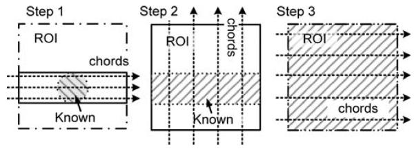
Illustration of the three-step chord reconstruction scheme.
IV. Numerical Experiments
In this section, numerical simulation and pre-clinical experiments and results are presented. First, we focus on the validation of the THT-SVD algorithm by showing a 1-D reconstruction test. Then we give 2-D reconstruction results on both simulated and real CT data.
A. 1-D Profiling
The proposed SVD-THT method is implemented on a single line. The four boundary points are a1 = −2.56, a2 = −1.0, a3 = 1.0, and a4 = 2.56. The ROI data g23(t) are obtained by computing the Hilbert transform of a predetermined function f(t) on (a1, a4). The function f(t) that contains 1024 samples is selected from a central column of the Shepp–Logan phantom. Also, g23(t) contains 400 samples.
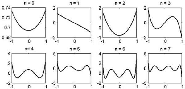
The required Sturm–Liouville problem is solved using a MATLAB toolbox called MATSLISE [23]. Because MATSLISE does not support singular boundary conditions [cf. (4)], the functions φn(t) are computed by solving the regular Sturm–Liouville problem with zero boundary conditions on the interval (a2 + ε, a3 − ε) where ε > 0 is sufficiently small. Visual comparisons of the eigen-functions computed using MATSLISE and the eigen-functions computed using a more accurate algorithm designed specifically for this problem showed almost no difference. Since the latter code was much more cumbersome and did not result in any noticeable gain of accuracy, we always used MATSLISE in our experiments. After the eigen-functions are computed, an orthonormality check is performed. Fig. 3 shows the first eight φn(t) calculated by MATSLISE. As one can see from the figure, eigen-functions with larger index n contain more high frequency information.
Fig. 3.
The first eight eigen-functions of the Sturm–Liouville problem. The boundary points are a1 = −2.56, a2 = −1.0, a3 = 1.0, and a4 =2.56.
By applying (19) g23(t) is projected onto each φn(t). During decomposition the total number of eigen-functions N can be chosen experimentally by taking into account noise level in the data, detector sampling rate, and the desired spatial resolution. A larger N can be used to recover smaller details for low noise data, while a smaller N is better for data with strong noise. For high accuracy we regard g23(t) as a continuous function, which can be obtained by performing linear interpolation between neighboring sampled pixels. Then all coefficients kn (n ≤ N) are computed.
The calculation of ψn is done by a continuous Hilbert transform instead of the FFT convolution method. Consider two neighboring sample points ti and ti+1. The contribution of φn(t) on the interval [ti, ti+1] to the Hilbert transform H23(φn)(x) can be expressed as
| (32) |
where
| (33) |
All ψn are normalized using (7). Finally, by applying (20) we get the interior ROI reconstruction without null space compensation. Results with two different choices of N are shown in Fig. 4, where (a) is the true profile. In (b) and (c) N equals 80 and 160, respectively. Next the null space compensation is performed. The minimization problem in (27)–(29) is solved using MATLAB Optimization Toolbox. The prior known subregion is the interval, [−0.1 0.1], which constitutes 10% of the total ROI width. The number of null space functions M is set to 10. Results are shown in Fig. 5: (a) is the true prfile; (b) and (c) are the compensated profiles with N = 80 and 160, respectively.
Fig. 4.

Reconstruction results by the SVD-THT without compensation using different number of eigen-functions N. (a) True profile. For (b) and (c) N equals to 80 and 160, respectively.
Fig. 5.

Reconstruction results by the SVD-THT with null space compensation using different number of eigen-functions N. (a) True profile. (b) and (c) Compensated profiles with N equals to 80 and 160, respectively. Location of prior known subregion is marked with a bold line segment in each panel.
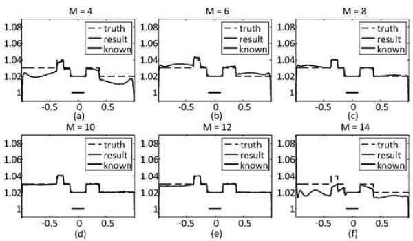
To test the robustness of the SVD-THT method, three different locations of the prior known subregion are chosen. They are[−0.35, −0.55], [−0.30, −0.10], and [0.35, 0.55]. The width of the known subregion is 0.2, which is also 10% of the total ROI range. The number of eigen-functions is set to N = 200, and the number of null space functions is set to M = 10. The results are shown in Fig. 6. Besides, two more tests are carried out. One is to demonstrate the in uence of the number of null space functions. Six groups of reconstructions with different M are compared. The prior known subregion is located in the center of the ROI and its width is 10% of the total ROI range. The results are given in Fig. 7. From (a)–(f), M is set to 4, 6, 8, 10, 12, and 14, respectively. The other is to investigate the stability with respect to the location of the ROI inside the object support. Three sets of boundary points are selected. The first set is the standard ROI con guration in which the boundary points are a1 = −2.56, a2 = −1.0, a3 = 1.0, and a4 = 2.56. In the other two sets the ROI area occupies a large portion of the object support or is close to the object boundary. The four boundary points for the second set are a1 = −2.56, a2 = −2.0, a3 = −0.4, and a4 = 2.56, and for the third set are a1 = −2.56, a2 = −2.0, a3 = 2.0, and a4 = 2.56. In each case the prior known subregion is assumed to be in the center of the ROI. The number of eigen-functions is set to N= 200 and the number of null space functions is set to M = 10. The reconstruction results are shown in Fig. 8.
Fig. 6.

Reconstruction results by the SVD-THT with null space compensation using different prior known subregions. From left to right: the known subregions are [−0.35, −0.55], [−0.30, −0.10], and [0.35, 0.55], respectively. The location of prior known subregion is marked with a bold line segment.
Fig. 7.
Reconstruction results by the SVD-THT with null space compensation using different number of null space functions M. From (a)–(f) M equals to 4, 6, 8, 10, 12, and 14, respectively. The location of prior known subregion is marked with a bold line segment.
Fig. 8.

Reconstruction results by the SVD-THT with null space compensation and different locations of the ROI. The boundary points are a1 = −2.56, a2 = −1.0, a3 = 1.0, and a4 = 2.56, in (a). In (b) they are a1 = −2.56, a2 = −2.0, a3 = 2.0, and a4 = 2.56. In (c) they are a1 = −2.56, a2 = −2.0, a3 = 2.0, and a4 = 2.56. The location of prior known subregion is marked with a bold line segment.
B. 2-D Numerical Simulation
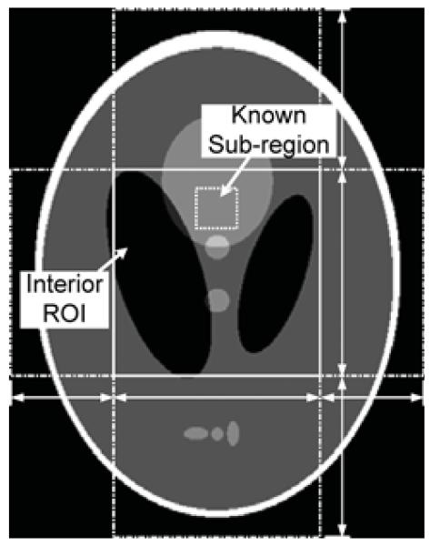
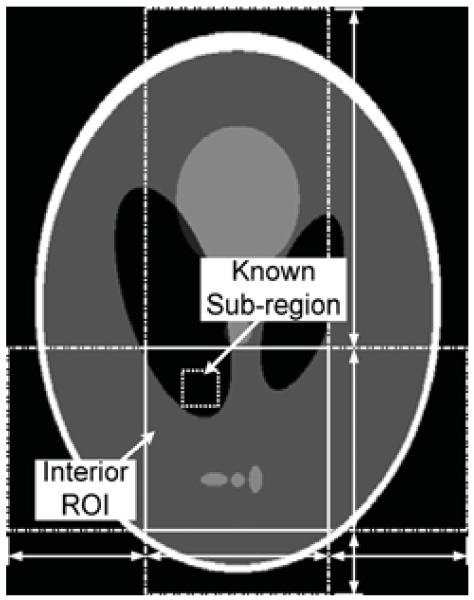
The 2-D numerical reconstruction is first verified using the well-known Shepp–Logan phantom. Similar to the previous section, the phantom is magni ed by a factor of 2.78. A rectangle of width 4.0 and height 5.12 is considered as the image support, and an interior ROI is defined inside the phantom. We assume that the interior ROI is a rectangle of size 2.0 × 2.0 located at the center of the image. A prior known subregion inside the ROI is selected whose size is 0.4 × 0.4. The configuration of the experiment is illustrated in Fig. 9, where the ROI region is marked with a solid rectangle and the prior known subregion is marked with a small dotted rectangle. The horizontal line segments with arrows indicate the four horizontal boundary points for the SVD-THT that are a1 = −2.0, a2 = −1.0, a3 = 1.0, and a4 = 2.0. The vertical line segments with arrows indicate the vertical boundary points that are a1 = −2.56, a2 = −1.0, a3 = 1.0, and a4 = 2.56.
Fig. 9.
An interior problem of the Shepp–Logan phantom. The gray scale window is [1.0, 1.05].
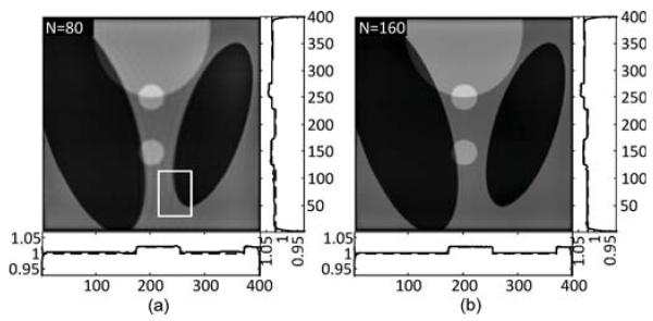
The projections are analytically generated based on the parameters of the phantom assuming a parallel beam geometry. The length of the detector array is 5.12, which consists of 1024 pixels. A total number of 1200 views are uniformly acquired in a range of 180°. During the course of projection simulation, only the rays passing through the ROI are computed. The DBP ROI data are calculated from the truncated sinogram. The boundary points for the horizontal and vertical chords are determined as shown in Fig. 9. In the compensation process, the number of null space functions is set to M = 8 for the two groups of chords. Finally, the SVD-THT with compensation is applied to obtain the ROI reconstruction. The results are shown in Fig. 10. The ROI image consists of 400 × 400 pixels of size 0.005 × 0.005 each. The number of eigen-functions N is set to 80 in (a) and 160 in (b). For each reconstruction two plots are drawn. One is along a vertical line and the other is along a horizontal line. Both of the lines pass through the ROI center. For each plot, the longer axis stands for the locations of image pixels, while the shorter axis stands for pixel values. On each plot the reconstructed result is shown as a solid curve, and the exact profile is shown as a dashed curve. Furthermore, the results are quantitatively evaluated in term of root mean square error (RMSE). The RMSE is calculated with respect to the true Shepp–Logan phantom using the central 90% of the ROI. This is done to avoid the singularity at the ROI boundary. The most notable effect of changing the value of N is the sharpness of edges. Hence, we also present a spatial resolution term, which is statistically estimated orthogonally across the edge of an ellipsoid as the full-width at half-maximum (FWHM) of the line response function tted into the Gaussian function [24], [25]. The edge that is used for calculation is marked by a white rectangle shown in Fig. 10(a). Quantitative results are listed in Table I.
Fig. 10.
The SVD-THT reconstruction results of the Shepp–Logan phantom from noise-free projections. The number of eigen-functions N is 80 in (a) and 160 in (b). In (a), the white rectangle indicates the subregion to measure the spatial resolution along the ellipsoid edge.
TABLE I.
Error Statistics for the Reconstructions in Fig. 10 in Terms of RMSE and Spatial Resolution
| Index | N | RMSE | Spatial resolution |
|---|---|---|---|
| (a) | 80 | 3.97×10⁻³ | 4.4×10⁻³ |
| (b) | 160 | 1.90×10⁻³ | 3.4×10⁻³ |
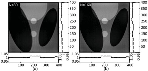
A major advantage of the SVD type methods is the stability with respect to noise. To test our method, reconstructions are performed from the noisy data. Following Fuchs [26], a 0.1% Gaussian noise is added to each of the original projection data sets as an acceptable approximation to Poisson noise in numerical simulations. The results are shown in Fig. 11. The number of eigen-functions N is 80 in (a) and 160 in (b). The gray scale window is [1.0, 1.05]. Similar to the noise-free tests, the RMSE and spatial resolution are quantitatively analyzed in each case, and the results are presented in Table II.
Fig. 11.
The SVD-THT reconstruction of the Shepp–Logan phantom from noisy projections. The number of eigen-functions N is set to 80 in (a) and 160 in (b).
TABLE II.
Error Statistics for the Reconstructions in Fig. 11 in Terms of RMSE and Spatial Resolution
| Index | N | RMSE | Spatial resolution |
|---|---|---|---|
| (a) | 80 | 3.50×10⁻³ | 6.0×10⁻³ |
| (b) | 160 | 4.04×10⁻³ | 3.7×10⁻³ |
C. Challenging Interior Problems
To evaluate the robustness of the proposed SVD-THT method, three challenging interior problems are tested. First, a new ROI inside the Shepp–Logan phantom is selected. The new ROI is very close to the phantom boundary. It is well known that the boundary of the Shepp–Logan phantom consists of a high density ring to simulate a human skull. However, the interior ROI mainly contains low density objects with very low contrast. This may challenge the algorithm stability and reconstruction accuracy. The new configuration is shown in Fig. 12. The four horizontal boundary points are a1 = −2.0, a2 = −0.8, a3 = 0.8, and a4 = 2.0. The four vertical boundary points are a1 = −2.56, a2 = −2.0, a3 = −0.4, and a4 = 2.56. The ROI region is marked with a solid rectangle with a size of 1.6 × 1.6. The prior known subregion is marked with a small dotted rectangle with a size of 0.32 × 0.32. The projections are analytically simulated in the same way as in Section IV-B. Reconstruction parameters are N = 160 and M = 8. Pixel size in the reconstructed image is 0.05 × 0.05.
Fig. 12.
Challenging interior problem on the Shepp–Logan phantom.
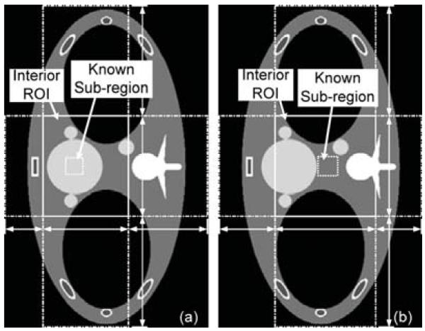
While the Shepp–Logan phantom mainly contains low contrast objects, high contrast objects such as bones and air cavities are commonly found in many clinical CT applications. In the presence of high contrast objects, it makes the reconstruction algorithms sometimes difficult to properly recover the soft tissues even when the projection data are not truncated. For the interior problems, the situation is even severe. To make the experiments more challenging, the FORBILD Thorax phantom [27] is also considered with two additional small disks in the heart [11]. The phantom is scaled down eight times to t into a 5.12 × 5.12 rectangle. For interior reconstruction two ROIs are selected as shown in Fig. 13. While the vertebra is excluded from the ROI but is located close to the ROI boundary in the configuration Fig. 13(a), part of the vertebra is covered in the configuration Fig. 13(b). In both configurations the low-density air cavities are partially covered. The prior known subregions are as follows. In (a) it is a 0.28 × 0.28 rectangle located close to the ROI boundary. In (b) it is a 0.32 × 0.32 rectangle located in the ROI center. All the boundary points are calculated before the reconstruction. For (a) the horizontal boundary points are a1 = −1.6, a2 = −1.0, a3 = 0.36, and a4 = 1.6, and the vertical boundary points are a1 = −2.56, a2 = −0.8, a3= 0.8, and a4 = 2.56. For (b) the horizontal boundary points are a1 = −1.6, a2 = −0.72, a3 = 0.88, and a4 = 1.6, and the vertical boundary points are a1 = −2.56, a2 = −0.8, a3 = 0.8, and a4 = 2.56. Projections are analytically simulated as in the Section IV-B, and the parameters are set as N = 360 and M = 6. A large N is used because of the high contrast objects, which require more eigen-functions to recover the sharp edges and reduce the Gibbs effect. The value of M is chosen experimentally. The pixel size of the reconstructed images is 0.05 × 0.05.
Fig. 13.
Two interior problems on the FORBILD Thorax phantom. The ROI regions are marked by solid rectangles. The prior known subregions are marked by small dotted rectangles. The horizontal and vertical line segments with arrows indicate the four boundary points for the SVT-THT method. The gray scale window is [0.92, 1.07].
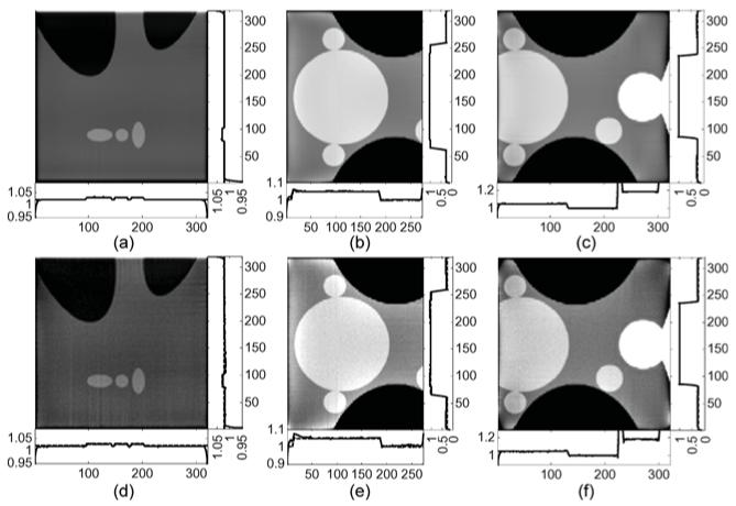
The results for the above three challenging interior problems are shown in Fig. 14, where (a) is the reconstructed image for the Shepp–Logan interior problem in Fig. 12, (b) is for the Thorax interior problem in Fig. 13(a), and (c) is for the Thorax interior problem in Fig. 13(b). In addition, reconstructions are repeated from noisy data. A 0.1% Gaussian noise is added to the original projections in the Shepp–Logan interior problem, and a 0.3% Gaussian noise is added to the Thorax interior problems. Corresponding results are shown in Fig. 14(d)–(f), respectively. For the reconstruction of (d) N = 120. And for (e) and (f) N = 280. The gray scale window for (a) and (d) is [0.95, 1.05]. The gray scale window for (b), (c), (e), and (f) is [0.92, 1.07].
Fig. 14.
SVD-THT reconstruction results of the problems defined in Figs. 12 and 13. (a)–(c) Noise-free reconstructions for Fig. 12 and Fig. 13(a) and (b), respectively. (d)–(f) Corresponding reconstructions from noisy data.
D. Preclinical Application
Thorax scans of a living sheep from a SIEMENS 64-slice CT scanner are employed to demonstrate the applications of the proposed algorithm (under the approval of Virginia Polytechnic Institute and State University IACUC committee). The thorax scans are necessary for pneumal and cardiac disease therapy and surgery assistance. Interior tomography will bring benefits to the related clinical applications as it can reduce X-ray dose. Two sets of projections are selected. One uses a normal dose protocol, and the other uses a low dose protocol. For the normal dose scan, the tube voltage and current are set to 100 kV and 150 mA. For the low dose scan the tube voltage and current were set to 80 kV and 17 mA. The scanning is in a typical fan-beam geometry after appropriate cone-beam weighting. The scanning radius is 570 mm. A total number of 1160 projections are uniformly acquired over 360°, and each projection contains 672 equiangular detector elements.
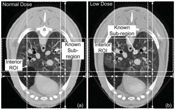
To construct an interior ROI problem, necessary preprocessing is performed on the original projection data. First, the projection data are rebinned from the fan-beam to parallel beam geometry, which allows a direct calculation of the Hilbert space data using (16). Then the ltered back-projection algorithm is used to obtain full reconstructions to serve as benchmarks for the interior problems. After that, the interior problems are specified as shown in Fig. 15. The reference images containing 1024 × 1024 pixels are reconstructed. The actual physical size of the image is 41.08 × 41.08 cm2. The ROI is located in the image center and has a size of 12.8 × 12.8 cm2 containing 320 × 320 pixels. For the normal dose scan, a small inner area of trachea is selected as a known subregion, whose actual size is 0.87 × 0.87 cm2 containing 22 × 22 pixels. We assume that the CT value inside the subregion is a constant and equals to the CT number of air. For the low dose scan, an inner area of an artery is selected. We assume that pixel values inside the subregion are known as an average value calculated from the FBP result. The actual size of the region is 1.14 × 1.14 cm2 and it contains 28 × 28 pixels. The boundary points for the SVD-THT method are determined in advance, and they are the same in both problems. Along the horizontal chords, they are a1 = −16.0, a2 = −8.0, a3 = 8.0, a4 = 16.0, and along the vertical chords they are a1 = −20.5, a2 = −8.0, a3 = 8.0, a4 = 20.5. All ai here are given in centimeters.
Fig. 15.
Two interior problems of real datasets from a sheep thorax perfusion study. (a) Normal dose data set and (b) low dose data set. The images are reconstructed by an FBP algorithm from the complete projection data. The gray scale window is [−1000 HU, 320 HU].
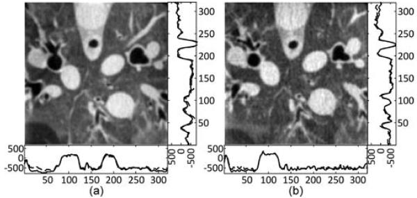
Once the interior ROIs are selected, the projection data are manually truncated accordingly. The SVD-THT reconstruction scheme is the same in both of the experiments with N = 160 and M = 6. The results are provided in Fig. 16, where (a) corresponds to the normal dose reconstruction, and (b) corresponds to the low dose reconstruction. The gray scale window for each result is set to [−1000, 320] HU.
Fig. 16.
The SVD-THT reconstructions from real CT data corresponding to the interior problems are defined in Fig. 15. The gray scale window is [−1000 HU, 320 HU].
E. Comparative Studies
To demonstrate the advantages of the proposed SVT-THT algorithm, comparative studies are performed with respect to a POCS-type algorithm. According to the work by Yu et al. [28], the implementation of the POCS-type algorithm consists of two major steps. In the first step the ordered-subset simultaneous algebraic reconstruction technique (OS-SART) is used to reconstruct an ROI image from truncated projection data. In the second step one performs iterative minimization of the L1 norm of the ROI gradient image. Note that all the results reconstructed by the POCS algorithm in this paper were added the constraint of the minimization of the L1 norm of the ROI gradient image. For a more detailed description please refer to the original paper. To deal with truncated data better, prior knowledge is utilized in order to improve stability [11], [12]. To make a fair comparison, the following prior knowledge is added: information about the object boundary, prior known subregion, and non-negativity. The additional constraints are imposed on the intermediate images after each L1 norm minimization step as follows. First, a new region is determined by enlarging 10% of the object boundary. All pixels outside this region are set to zero. Second, the values inside the prior known subregion are set to the known (or estimated) values. Finally, all negative values in the intermediate image are set to zero. Besides, the parameters are adjusted for each interior problem for a best performance.
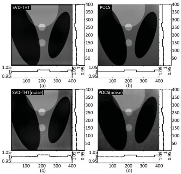
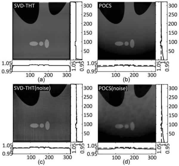
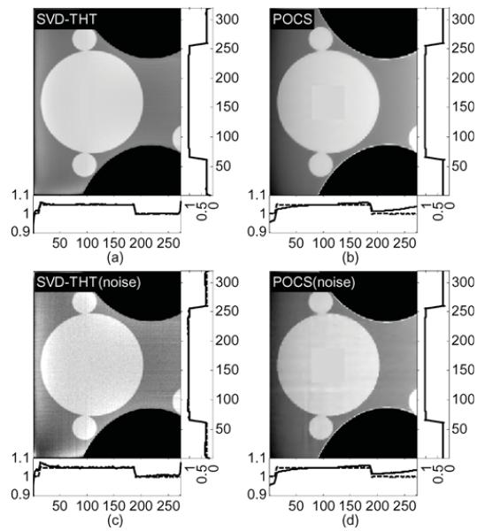
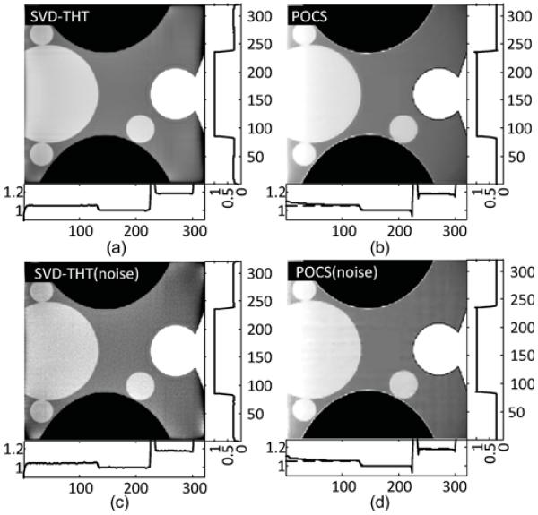
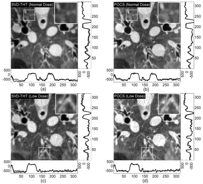
The interior problems described in the previous subsections are tested. Among them four are based on the phantoms and two are based on real CT data. For numerical phantoms, reconstructions from noise-free and noisy projections are compared. All reconstruction results are shown and compared in multiple gures. The reconstructions of the Shepp–Logan phantom are shown in Figs. 17 and 18. The reconstructions of the Thorax phantom are shown in Figs. 19 and 20. The results with real CT data are presented in Fig. 21.
Fig. 17.
Reconstruction result comparisons for the Shepp–Logan interior problem defined in Fig. 9.
Fig. 18.
Reconstruction result comparisons for the Shepp–Logan interior problem defined in Fig. 12.
Fig. 19.
Reconstruction comparisons for the Thorax interior problem defined in Fig. 13(a).
Fig. 20.
Reconstruction comparisons for the Thorax interior problem defined in Fig. 13(b).
Fig. 21.
Reconstruction comparisons of real sheep thorax study data sets for the interior problems defined in Fig. 15. The gray scale window is set to [−1000, 320] (HU). The images indicated by the dashed rectangles are magnified in the top-right corner to emphasize the difference between the results reconstructed by the SVD-THT and POCS.
V. Discussions and Conclusion
From Fig. 4, it is noticeable that the reconstructed profile is smoother in (b) than in (c). It may be concluded from the comparison that when N increases, more high frequency details such as sharp edges can be found, i.e., the recovery of high frequency information is improved. This phenomenon is especially visible in Fig. 5, where the compensated profiles are plotted. We notice also that the reconstructions suffer from the prominent Gibbs effect with a smaller N. For the specific case of our numerical results, we suggest that N should be chosen no less than 160.
The results in Fig. 6 show that the proposed null space compensation is capable of recovering the missing information about an ROI aided by a prior known subregion. The compensated profiles are close to the exact ones in most of the ROI. However, the reconstruction accuracy decreases in places which are far away from the known subregion and close to the ROI boundaries. This is caused by the sharp DBP data truncation at the ROI boundaries.
The results in Fig. 7 illustrate how the total number of null space functions M affects the compensation. It can be seen that a proper choice of M is important. When M is too small, the few functions cannot adequately represent the null space, resulting in a biased profile. On the other hand, when M is too large, there are too many unknowns in (27) and the stability of compensation becomes poor. As a result oscillations may occur (see the case M = 14). In our experiments a proper choice of M is between 8 and 12. The reconstructions with different locations of the ROI in Fig. 8 show the reconstructions are stable in all three cases. The change of the ROI location makes little or no in uence on the performance of the proposed method.
Next let us discuss the 2-D image reconstruction experiments. It can be seen from Fig. 10 that the inner ROI area of the Shepp–Logan phantom is accurately reconstructed. There are no obvious artifacts in the ROI center, and dropdowns can be found close to the ROI boundaries. The reason is that small intervals of length δ are excluded from the optimization in (27) to reduce the in uence of boundary singularities. The effect of different choices of N can also be well demonstrated in Fig. 10. Blurred edges can be seen in Fig. 10(a) where N equals 80. The Gibbs effect is also visible in the image. However, the edges are sharper in Fig. 10(b) where N = 160. This observation is consistent with the quantitative results in Table I. According to Table I, the RMSE is reduced by 52% and the spatial resolution is increased from 4.4 × 10⁻³ to 3.4 × 10⁻³ when N is changed from 80 to 160. In Fig. 11, when noise is added to the original projection data, the results suffer from noise and artifacts. As expected, image quality decreases farther away from the known subregion. Because the known subregion is located close to the upper boundary of the ROI, noise leads to a larger bias on the opposite side of the image. In the regions close to the known subregion, image values are stable. Comparing the results with different N we infer that decreasing the number of eigen-functions can reduce noise and make the whole ROI more uniform. Based on the data in Table II, when N = 80 the RMSE is 87% of that of N = 160. A smaller N improves stability. On the other hand, spatial resolution decreases when N decreases. When N = 160, image resolution is higher. In summary, a balance between stability and spatial resolution is achievable by adjusting N. From the additional interior reconstructions in Fig. 14, it can be seen that the SVD-THT method is sufficiently robust. It accurately recovers both low and high contrast features inside the ROI. Moreover, it can be seen from Fig. 14(b) and (c) that the presence of high contrast features does not lead to artifacts regardless of whether the former are located inside or outside the ROI. With noisy data, image quality decreases somewhat, especially near the ROI boundaries. However the central area remains stable.
Fig. 16 shows the reconstruction results from real preclinical CT data. Blood vessels, tracheas and other organs are clear and discriminable. For the normal dose data, a large N is used to for high spatial resolution. For the low dose data, N is reduced to improve stability and suppress noise. Besides, two different known subregions are tested. In Fig. 16(a), the known subregion contains only air, whose CT value is accurately known and remains constant throughout the subregion. In Fig. 16(b), the known subregion is inside an artery, whose uniformity is only approximate. In the experiment, we assume that its CT value is nevertheless constant and equals to some averaged value. Image quality is good in both cases. Sometimes a prior known subregion with a constant CT number is not easy to nd, because air, water, or other highly uniform media do not exist anywhere inside the animal or human body. As an alternative choice, a relatively smooth area such as soft tissue, a large artery, or vein can be chosen. Additionally, the size of the known subregion is important because a larger one will result in higher stability and lead to better interior reconstruction.
The experimental results shown in Figs. 17–21 demonstrate the advantages of our SVD-THT method. There are biases in some of the POCS results, especially in Fig. 18 where the ROI is close to the object boundary and the biases are noticeable at the bottom of the ROI. What is more, in Fig. 19(b) and (d), an intensity gradient can be seen from the horizontal profile at the bottom of the images. In Fig. 17(d), a small gradient can be observed from the vertical profile on the right of the image. These gradients are found in ROIs which are located away from the center of the object support. The more one-sided a ROI is, the more prominent the gradient becomes. Besides, the existence of high density objects can strongly affect the reconstruction results. Comparing the POCS results in Figs. 19 and 20, the gradient effect in Fig. 20 is much smaller than that in Fig. 19. Yet the main difference between the two problems is the location of the vertebra. The vertebra is excluded from the ROI in Fig. 19, while most of the vertebra is included in the ROI in Fig. 20. This indicates that a high density object outside the ROI degrades the image quality of the POCS reconstruction results. On the other hand, biased values can be seen only close to the edge of the ROI in the results reconstructed by the SVD-THT method, while stable image can be found in most of the ROI. Compared to the POCS method, location of high density objects relative to the ROI has much smaller influence on the proposed method. This is because the proposed SVD-THT method does not need to reconstruct the object outside the ROI. POCS methods reconstruct the entire object, both inside and outside the ROI. Hence any error in the recovery of a high density object outside the ROI results in significant artifacts inside the ROI. The real data reconstruction results are compared in Fig. 21. The SVD-THT method tries to balance the noise stability and detail preservation. According to the theory of L1 norm minimization [29], the POCS reconstruction reduces image noise by finding a solution with minimum L1 norm of its gradient. As a result the reconstructed images have some blocky effects [see the local magnifications located in the upper-left corner of each ROI result in Fig. 21, and also Fig. 17(d) and Fig. 18(d)]. For practical interior CT imaging, the presence of noise is inevitable and it makes the problem more challenging. As discussed above, several additional factors may influence the reconstruction stability such as the ROI location relative to high density features inside the object. To suppress these interferences, more iterations and more prior information are needed for the POCS based methods. However, our SVD-THT method does a better job without either increasing computation cost or taking into account additional prior knowledge.
In conclusion, a new SVD algorithm is proposed for interior tomography. Both numerical simulation and preclinical experiment results demonstrate the reconstruction capability. The reconstruction results show high stability under some critical conditions even with noise. Because interior tomography is a general approach, which can help to reduce radiation dose and suppress scattering artifacts we believe that the proposed algorithm may have a significant impact on the preclinical/clinical CT applications and be extended to some other tomographic modalities such as SPECT, PET, etc.
Acknowledgments
This work was supported in part by the National Natural Science Foundation of China (NNSFC) under Grant 60871084 and Grant 10905030, in part by the Beijing Natural Science Foundation (research on key techniques of medical cone-beam CT reconstruction from little data based on compressed sensing theory), in part by the National Science Foundation/Major Research Instrumentation (NSF/MRI) program (CMMI-0923297), and in part by the National Institutes of Health (NIH) under Grant (EB011785). The work of A. Katsevich was supported by NSF under Grant DMS-0806304 and Grant DMS-1115615.
Contributor Information
Xin Jin, Department of Engineering Physics, Tsinghua University and Key Laboratory of Particle and Radiation Imaging (Tsinghua University), Ministry of Education, Beijing 100084, China.
Alexander Katsevich, Department of Mathematics, University of Central Florida, Orlando, FL 32816 USA.
Hengyong Yu, Biomedical Imaging Division, VT-WFU School of Biomedical Engineering and Sciences, Virginia Tech, Blacksburg, VA 24060 USA; Wake Forest University Health Sciences, Winston-Salem, NC 27157 USA.
Ge Wang, Biomedical Imaging Division, VT-WFU School of Biomedical Engineering and Sciences, Virginia Tech, Blacksburg, VA 24060 USA; Wake Forest University Health Sciences, Winston-Salem, NC 27157 USA.
Liang Li, Department of Engineering Physics, Tsinghua University and Key Laboratory of Particle and Radiation Imaging (Tsinghua University), Ministry of Education, Beijing 100084, China.
Zhiqiang Chen, Department of Engineering Physics, Tsinghua University and Key Laboratory of Particle and Radiation Imaging (Tsinghua University), Ministry of Education, Beijing 100084, China.
References
- [1].Yu HY, Ye YB, Wang G. “Interior tomography: Theory, algorithms and applications,”; Proc. SPIE; 2008.p. 70780F. [Google Scholar]
- [2].Louis AK, Rieder A. “Incomplete data problems in X-ray computerized tomography,”. Numer. Math. 1989;56(4):371–383. [Google Scholar]
- [3].Maass P. “The interior Radon transform,”. SIAM J. Appl. Math. 1992;52(3):710–724. [Google Scholar]
- [4].Faridani A, Ritman EL, Smith KT. “Local tomography,”. SIAM J. Appl. Math. 1992;52(2):459–484. [Google Scholar]
- [5].Katsevich AI, Ramm AG. “New methods for finding values of the jumps of a function from its local omographic data,”. Inverse Probl. 1995;11:1005–1023. [Google Scholar]
- [6].Faridani A, et al. “Local tomography II,”. SIAM J. Appl.. Math. 1997 Aug;57(4):1095–1127. [Google Scholar]
- [7].Natterer F. “The mathematics of computerized tomography,”. Soc. Indust. Math. 2001 [Google Scholar]
- [8].Defrise M, et al. “Truncated Hilbert transform and image reconstruction from limited tomographic data,”. Inverse Probl. 2006;22:1037–1053. [Google Scholar]
- [9].Ye YB, et al. “A eneral local reconstruction approach based on a truncated Hilbert transform,”. Int. J Biol. Imag. 2007:8. doi: 10.1155/2007/63634. [DOI] [PMC free article] [PubMed] [Google Scholar]
- [10].Ye YB, Yu HY, Wang G. “Exact interior reconstruction with cone-beam CT,”. Int. J Biol. Imag. 2007:5. doi: 10.1155/2007/10693. [DOI] [PMC free article] [PubMed] [Google Scholar]
- [11].Kudo H, et al. “Tiny a priori knowledge solves the interior problem in CT,”. Phys. Med. Biol. 2008;53:2207–2231. doi: 10.1088/0031-9155/53/9/001. [DOI] [PubMed] [Google Scholar]
- [12].Courdurier M, et al. “Solving the interior problem of computed tomography using a priori knowledge,”. Inverse Probl. 2008;24:065001. doi: 10.1088/0266-5611/24/6/065001. [DOI] [PMC free article] [PubMed] [Google Scholar]
- [13].Li L, et al. “A general region-of-interest image reconstruction approach with truncated Hilbert transform,”. J. X-ray Sci. Tech. 2009;17(2):135–152. doi: 10.3233/XST-2009-0218. [DOI] [PubMed] [Google Scholar]
- [14].Gel’fand IM, Graev MI. “Crofton’s function and inversion formulas in real integral geometry,”. Funct. Anal. Appl. 1991;25(1):1–5. [Google Scholar]
- [15].Ye YB, Yu HY, Wang G. “Gel’fand-Graev’s reconstruction formula in the 3D real space,”. Med. Phys. 2011;38(7):S69–S75. doi: 10.1118/1.3577765. [DOI] [PMC free article] [PubMed] [Google Scholar]
- [16].Noo F, Clackdoyle R, Pack JD. “A two-step Hilbert transform method for 2-D image reconstruction,”. Phys. Med. Biol. 2004;49:3903–3923. doi: 10.1088/0031-9155/49/17/006. [DOI] [PubMed] [Google Scholar]
- [17].Xu Q, Mou XQ, Wang G. “Statistical interior tomography,”. IEEE Trans. Med. Img. 2011 May;30(5):1116–1128. doi: 10.1109/TMI.2011.2106161. [DOI] [PMC free article] [PubMed] [Google Scholar]
- [18].Yu HY, Ye YB, Wang G. “Interior reconstruction using the truncated Hilbert transform via singular value decomposition,”. J. X-ray Sci. Tech. 2008;16(4):243–251. [PMC free article] [PubMed] [Google Scholar]
- [19].Katsevich A. “Singular value decomposition for the truncated Hilbert transform,”. Inverse Probl. 2010;26:115011. [Google Scholar]
- [20].Katsevich A. “Singular value decomposition for the truncated Hilbert transform: Part II,”. Inverse Probl. 2011;27:075006. [Google Scholar]
- [21].Gakhov FD. Boundary Value Problems. Pergamon; Oxford, U.K.: 1966. [Google Scholar]
- [22].Okada S, Elliot D. “The nite Hilbert transform in L2,”. Math. Nachr. 1991;153:43–56. [Google Scholar]
- [23].Ledoux V, Daele MV, Berghe GV. “Matslise: A Matlab package for the Numerical Solution of Sturm-Liouville and Schrödinger equations,”. ACM Trans. Math. Soft. 2005;31(4):532–554. [Google Scholar]
- [24].Wang G, Yu H, Ye Y. “A scheme for multisource interior tomography,”. Med. Phys. 2009;36(8):3575–3581. doi: 10.1118/1.3157103. [DOI] [PMC free article] [PubMed] [Google Scholar]
- [25].Schlueter FJ, et al. “Longitudinal image deblurring in spiral CT,”. Radiology. 1994;193(2):413–418. doi: 10.1148/radiology.193.2.7972755. [DOI] [PubMed] [Google Scholar]
- [26].Fuchs T. Simulation of noise [Online] Available: http://www.imp.uni-erlangen.de/phantoms/noise/noise_sim.htm.
- [27].Sourbelle K. Thorax phantom [Online] Available: http://www.imp.uni-erlangen.de/phantoms/thorax/thorax.htm.
- [28].Yu H, Wang G. “Compressed sensing based interior tomography,”. Phys. Med. Biol. 2009;54:2791–2805. doi: 10.1088/0031-9155/54/9/014. [DOI] [PMC free article] [PubMed] [Google Scholar]
- [29].Candes E, Romberg J, Tao T. “Robust uncertainty principles: Exact signal reconstruction from highly incomplete frequency information,”. IEEE Trans. Inf. Theory. 2006 Feb;52(2):489–509. [Google Scholar]


