Methods of MRI-Based Structural Imaging in the Aging Monkey

Abstract

Rhesus monkeys, whose typical lifespan can be as long as 30 years in the presence of veterinary care, undergo a cognitive decline as a function of age. While cortical neurons are largely preserved in the cerebral cortex, including primary motor and visual cortex as well as prefrontal association cortex there is marked breakdown of axonal myelin and an overall reduction in white matter predominantly in the frontal and temporal lobes. Whether the myelin breakdown is diffuse or specific to individual white matter fiber pathways is important to be known with certainty. To this end the delineation and quantification of specific frontotemporal fiber pathways within the frontal and temporal lobes is essential to determine which structures are altered and the extent to which these alterations correlate with behavioral findings. The capability of studying the living brain non-invasively with MRI opens up a new window in structural-functional and anatomic-clinical relationships allowing the integration of information derived from different scanning modalities in the same subject. For instance, for any particular voxel in the cerebrum we can obtain structural T1-, diffusion- and magnetization transfer-magnetic resonance imaging (MRI) based information. Moreover, it is thus possible to follow any observed changes longitudinally over time. These acquisitions of multidimensional data in the same individual within the same MRI experimental setting would enable the creation of a data base of integrated structural MRI-behavioral correlations for normal aging monkeys to elucidate the underlying neurobiological mechanisms of functional senescence in the aging non-human primate.

Introduction

Studies of normal aging using the rhesus monkey as an animal model have shed new light on the aging process. Using morphological methods ranging from standard light microscopy to electron microscopy has demonstrated that normal aging in the forebrain is characterized by dramatic changes in white matter while gray matter is largely preserved. Specifically, studies have demonstrated that cortical neurons are not lost with age although there are changes in cortical neuropil such as thinning in layer 1 and mild dendritic atrophy (1, 2). In contrast there are major changes in forebrain subcortical white matter including ubiquitous breakdown of the integrity of the myelin sheaths of axons (1, 3) and a reduction in axon numbers (4). These changes are thought to be the underlying neurobiological correlate of the overall volume reduction in white matter as documented by MRI (magnetic resonance imaging) (2, 5) and cognitive decline that occurs with aging (6-8). Anatomical studies in humans also indicate that neuron numbers are preserved in the cerebral cortex (9-11), while white matter is lost (12). While these types of histological examinations are critical for examining the microstructures of the brain, because they are so labor intensive, they can only sample limited brain regions. Consequently, whether the myelin breakdown is diffuse or is topographically specific both in temporal appearance and in severity is an open question. Unlike morphogical studies using post-mortem tissue samples, MRI allows the non-invasive, in vivo assessment of many different brain parameters including the topography and volume of gray and white matter brain structures. Moreover, as discussed below, newer imaging modalities allow for the assessment of a wide variety of tissue properties beyond simple morphology.

MRI Protons are the most commonly used nuclei for MR in medical imaging. Through the use of radiofrequency pulses and manipulations of static and dynamic magnetic fields, signals can be received and localized from protons in the body (13, 14). These signals are turned into spatial images, which characterize the contribution from each ‘voxel’ (volume element). Much of the utility of MR imaging arises from the array of properties that this signal can be made to highlight. These include the intrinsic magnetic properties of tissue, such as relaxation times (T1, T2) and proton density (13, 14). The macroscopic and microscopic movements of protons can also be detected, providing the basis for depiction of circulation, including angiography (15) and tissue perfusion parameters such as blood flow and blood volume (16-18), as well as diffusion characteristics (19-21). Since MR signal is modulated by the local magnetic field that the protons experience, tissue properties that alter the local magnetic field can be detected, including variations in blood oxygenation state (22) and the chemical composition of tissue (for example, protons that are contained in water experience a different local magnetic field than protons that are contained in fat, etc.) (23-25). All of these MR signal sensitivities can be used to create images that reveal distinctive characteristics of tissue. New or revised imaging protocols are continually being developed which are sensitive to additional properties of brain tissue, with an enlarging repertoire of potential clinical and research applications.

Multimodal Imaging While morphometric methods using T1-weighted images have been extremely useful for morphometric investigations focused on precise volumetric changes of detailed brain anatomy over time, the integration of morphometry with other imaging modalities has opened a novel window for neuroscience allowing investigation of the living brain (24). For example, in the aging monkey brain, white matter changes including myelin defects and loss of myelinated fibers would be predicted to result in modified water diffusivity, and hence alterations in fractional anisotropy (FA). DT-MRI (diffusion tensor-MRI) is sensitive in these changes, facilitating mapping of degenerating fiber tracts as a function of age. Thus, the combination of morphometry with DT-MRI offers a unique opportunity to study white matter fiber tract anatomy, in addition to cortical and subcortical gray matter structure. The combined use of T1-MRI morphometry, DT-MRI and magnetization transfer MRI (MT-MRI), are important assets for the correlation with behavioral measures and the study of structure-function relationships.

Future Directions Magnetic resonance technologies have introduced a new set of tools for capturing features of normal brain anatomy and function in living monkeys. Quantitative applications remain a work in progress, but represent a vast, untapped source of biologically relevant information (26-28). As such these tools have begun to revolutionize the way we view the brain – both literally and figuratively – as well as our expectations for future investigative possibilities. In the following sections we survey the methodologies for T1-based morphometric analysis, diffusion imaging (including two distinct techniques, namely a) DT-MRI, and b) high angular resolution diffusion imaging (HARDI)), MT-MRI as well as applications of some of these techniques to studies of the aging monkey brain.

Methodology

Monkey Brain Scanning For image acquisition, monkeys are anesthetized with a mixture of ketamine and xylazine and the head stabilized in the coronal stereotactic plane using a specially designed stereotactic machine constructed from lexan and brass or alternatively, lexan alone, which effectively avoids interfering with image acquisition (29). This allows the monkey's head to be completely stabilized in the scanner, eliminating movement artifact. It also allows reliable positioning in the exact same coronal stereotactic orientation in the scanner for subsequent scanning sessions. This dramatically simplifies alignment and registration of different scan sequences both within and between scanning sessions. This is an especially important consideration for longitudinal studies. It also standardizes the orientation between subjects within the limits of standard stereotactic variability. A full scanning protocol can include up to five different scanning modalities in a single 2 hour scanning session. In addition to the ability to anesthetize and reproducibily stabilize the brain, use of non-human primate subjects also allows scans to be repeated within one or two weeks, if upon analysis, any of the scans prove to have unaccepatable artifacts.

Image acquisition

A) T1-, T2-, and Proton density-weighted MRI State-of-the art MRI provides a degree of anatomic detail that allows both the detection of structures of the brain and the measurement of their volumes (30). Given its relative non-invasiveness and anatomic resolution, MRI has become the method of choice for neuroanatomic evaluation and morphometric analysis. MRI's success in neuroimaging results in part from the wide variety of tissue properties to which the MRI acquisition can be made sensitive. Usually, MR imaging is designed to take advantage of the differences in T1 (longitudinal relaxation time), T2 (transverse relaxation time), and differences in the intrinsic proton density found between gray matter, white matter, and cerebrospinal fluid (CSF) (Figure 1).

Figure 1.

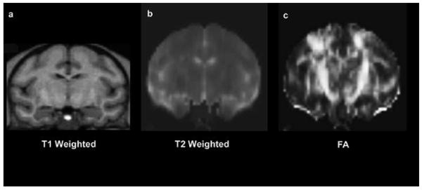
Example coronal MR images showing in the same subject (a) T1 (longitudinal relaxation time), (b) T2 (transverse relaxation time), and (c) Fractional Anisotropy (FA) map in a rhesus monkey brain. Note the contrast differences between the gray matter, white matter and cerebrospinal fluid (CSF).

B) Diffusion Imaging

B₁ Diffusion Tensor MRI Beginning in the mid-1940s development of diffusion tensor imaging (DT-MRI) has progressed rapidly including both, technological advances (31-38) and anatomical applications (20, 21, 39-42). DT-MRI measures the three-dimensional self-diffusion of water. From the DT-MRI data there are derived scalar metrics such as fractional anisotropy (FA) and lattice anisotropy (LA). FA, the mostly used of the two metrics, is a calculated measure from DT-MRI data that is dependent on the orientational coherence of the diffusion compartments within a voxel and provides an index of white matter restrictional microstructure (39). In brain white matter, diffusion is largely restricted by the axonal projections and would occur primarily in a single orientation in highly anisotropic (i.e., highly oriented) regions of the brain such as the stems (compact portion) of the major fiber tracts. In contrast, regions that are less organized in a single orientation (i. e., more isotropic) provide less structured restriction of the molecules. An example of an anisotropic cerebral region is the stem of the corticospinal tract, which constitutes much of the posterior limb of the internal capsule; instead, a more isotropic region is the corona radiata where crossing of the axons of different fiber tracts occurs. The FA metric assesses biophysical properties that affect FA, such as axonal density, myelination and orientation coherence, within the fiber tracts (43). The FA has a value of 0 for isotropic diffusion (e.g. minimally organized restriction in a single orientation as in regions with crossing fibers) and a value of 1 for maximally anisotropic diffusion (e.g. maximally organized restriction in a single orientation as in the internal capsule) (Figure 1). Experimentally observed differences in FA values of similar anatomical regions between groups of animals would suggest a difference in the white matter microenvironment. For example, lower fiber density or decreased directionality would result in less tightly packed fiber bundles, and thus, water diffusion would be less restricted and FA values would be lower. FA has been used to examine changes in the white matter in clinical studies of multiple sclerosis (44), schizophrenia (45), alcoholism (46, 47), amyotropic lateral sclerosis (48), and other degenerating conditions.

Recent studies have also documented significant declines in the orientational organization of the white matter in normal and pathological aging, suggesting that DT-MRI may be a useful tool for the study of brain aging (49-52). From a morphological anatomic perspective, DT-MRI analysis enables us to characterize the stem of a white matter fiber pathway in terms of its orientation, location and size. To date DT-MRI fiber tract analysis has been performed in two different ways. Using manual or model-independent methods by which we can derive the trajectory of the stem of a fiber bundle and approximate its extreme peripheries using segmentation (20, 53, 54). This direct, manual, slice-by-slice segmentation based method has been named the “color-map approach” (53, 55). A different, automated tractographic approach by which we can trace efficiently the stem of a fiber pathway, uses mathematically driven model-based methods (56, 57). Although the field of DT-MRI-based brain tractography is expanding rapidly with impressive results, it has to be pointed out that there are still some conceptual obstacles to overcome and in this stage we can only identify and characterize the stems of the major fiber tracts with reliability (20, 55, 58). Moreover, the solution to the problem of elucidating the sprays and the extreme peripheries of the bundles has not yet been solved completely (59, 60). Therefore, when we use the term pathway, tract or bundle, as analyzed by DT-MRI in the present study, we refer commonly to its stem, i.e., the compact portion of the fiber tract where the axons course together (as opposed to the tract's spray, origins and terminations) (20).

B₂ High angular resolution diffusion imaging (HARDI) HARDI is used to refer to diffusion spectrum imaging (DSI) and Q-ball imaging (QBI). The use of HARDI techniques aims to overcome limitations of DT-MRI in extracting information of white matter architecture (60-63). Specifically, QBI and DSI allow the delineation of multiple orientations within a voxel, a property that has been applied to such white matter regions as the corona radiata where fibers are crossing. QBI is a HARDI method capable of resolving complex, intravoxel white matter heterogeneity. Investigators have recently validated the QBI reconstruction in a rayon fiber phantom (64) and separately in a phantom constructed from excised rat spinal cord (65). Recently, there has been developed a method combining DT-MRI with QBI, i.e., multiple waveform fusion (MWF) (66). Tractography can be also performed using HARDI data.

C) Magnetization Transfer MRI MT-MRI was originally described by Wolff and Balaban (67, 68). This method has been proven useful for following demyelination and lesions where demyelination occurs such as in multiple sclerosis. One publication examined the effects of myelin injury versus demyelination. These authors concluded that changes in a quantity termed the magnetization transfer ratio (MTR) were much smaller in the case of myelin injury compared to frank demyelination - thus the predominant MT effect in white matter may be attributable to the amount of myelin (69). Other investigators, though, have found nice correlations between histopathologic metrics of diffuse axonal injury and MTR (70). Thus, an exact interpretation of the meaning of changes in white matter MTR is an open question. Nonetheless, MT imaging may offer the potential for quantifying changes in myelination that might occur as a function of aging.

A number of publications have examined the effect of aging on the white matter MTR in humans, and most of these studies have shown that there is a decrease in MTR as a function of age (71-73). However, a few studies (74) have shown no difference. This variability in results might be due to the difference in sequence parameters used as well as small effect sizes, partial volume averaging and differences in neuroanatomical interpretation.

Quantification

A) Image Registration

Image Registration is commonly necessary to facilitate calculations of derived parametric maps (i.e. diffusion tensor, magnetization transfer), to increase signal to noise ratio by averaging of multiple acquisitions, and to integrate information across modalities of imaging and between individual subjects. Image registration can be intra-subject, involving repeated images of the same subject or inter-subject, involving registration of images between different subjects to facilitate comparisons. In general, image registration for the studies presented here is performed using the FSL-FLIRT software package (75, 76). This tool invokes a linear (affine) registration based upon image intensity similarity maximisation. This tool can be used both intra- and inter-subject, as well as within and between imaging modalities. The representation of the neocortex is particularly complex, due to its constrained topology and highly curved topography and inter-individual variability. This complexity can lead to registration errors, which are inherently present in all procedures involving inter-subject mapping. Limitations are due in part to the finite number of degrees of freedom allowed in the transformation procedure, as well as the ill-posed nature of inter-subject correspondence in topology with respect to detailed topography and function. The ultimate sensitivity of a method is constrained to identification of regions of change that are large with respect to limitations in the precision of linear registration procedures arising from inter-subject anatomic variability.

B) Morphometric Analysis

The quantification of morphometric properties is a valuable adjunct in the interpretation of MR images. This approach takes advantage of the digital nature of the MR image, and its utility for computerized image analysis. There are many morphometric properties of normal and pathologic structures that are perceptually apparent to the human observer. To this end, quantification of properties such as volume (size), shape, location, and intensity characteristics within a region have found utility for many classes of structural analysis (77).

Structures are observed in an image based on regions of intensity, homogeneity, and similarity. Different contrast mechanisms for MR images result in the identification of different types of structures. In images with T1 contrast, for example, image intensity provides good differentiation (i.e. contrast) between the gray matter, white matter and cerebrospinal fluid (CSF) compartments of the brain. This anatomic structure-based contrast makes these types of images useful for the quantification of anatomic structure. Other MR images (those with T2 contrast, for example) often show markedly contrasting signal intensity differences in the transition between normal tissue and that which is diseased or damaged (i.e. some tumors, infarction, infections, etc.). Such images are particularly suitable for the quantitative characterization of the volumetric extent of the pathologic process.

The entire monkey brain can be segmented morphometrically into discrete regions of interest or parcellation units (PUs) including general (gross) segmentation, and individually tailored, topographically defined parcellation methods applied to subcortical nuclei and brainstem. In addition, the neocortex can be subjected to a further analysis into fine-grained neuroanatomic units applied to the cerebral cortex. Quantification of alterations at local and whole-brain levels can be accomplished. This morphometric system uses the volumetric method developed at the Center for Morphometric Analysis. This complex method has been developed over eighteen years and has been applied extensively to multiple study populations (78-81). This system, which was originally developed for the human brain is here modified and adapted to the monkey brain. It consists of the segmentation of the different brain structures followed by parcellation of the neocortex as described in detail in the following.

Segmentation is the process of delimiting homogeneous regions using classification and labeling procedures. Segmentation, as a topic in imaging science, radiology, computer vision, etc., has a long and rich literature. A number of comprehensive reviews provide a detailed overview of this topic (82, 83). Segmentation is a necessary precursor to quantitative regional morphometric treatments as introduced above. The specific procedures used for segmentation will depend on the nature of the image intensity information. In addition to the input image itself, segmentation procedures typically take advantage of derived features such as edge information, textures, spatial variation in illumination, etc. (84). Segmentation may also depend in part on manual or automated knowledge-based judgments regarding inter-structural boundaries (85, 86). User input is often (but not always) required for segmentation to provide training data, establish parameters, or to verify/modify the resultant regions. Methodologies have been developed which allow brain segmentation based on many types of neuroanatomic description. Typical anatomic divisions include the forebrain, brainstem, and cerebellum. The ventricular system can be also segmented into lateral ventricles, third ventricle and fourth ventricle. The forebrain can further be segmented by standard algorithms into cerebral cortex, cerebral white matter, caudate nucleus, nucleus accumbens septi, putamen, globus pallidus, thalamus, basal forebrain, hypothalamus, peduncular tegmentum, posterior-ventral diencephalic region (containing the red nucleus and the subthalamic nucleus), hippocampus, and amygdala (80, 87).

Cortical parcellation is a system of subdivisions of the cerebral cortex. This is performed using dedicated software, which allows the principal cerebral cortical gyri to be parcellated by a semi-automated method into twenty-five regions of interest or parcellation units (PUs) per hemisphere, with reference to a set of anatomical landmarks and the course of fissures as shown in Figures 4c and 5 (78, 88). The parcellation operation is initiated after the brain has been segmented into gray matter and white matter compartments. The segmented cortex is defined superficially by a contour at the cerebral surface and by a contour at the cortex-central white matter boundary. The cortex, thus delimited and ready for parcellation, is a continuous ribbon at the outer margin of the hemisphere.

Figure 4.

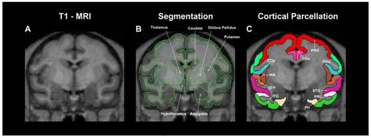
Example illustration showing the result of segmentation (middle) and cortical parcellation (right) in a coronal MRI section of the monkey cerebrum. Abbreviations: CGa: anterior cingulate gyrus; ITG: inferior temporal gyrus; PH: parahippocampal gyrus; POG: postcentral gyrus; PRG: precentral gyrus; PRL: prelunate gyrus; STG: superior temporal gyrus; STP: supratemporal plane.

Figure 5.

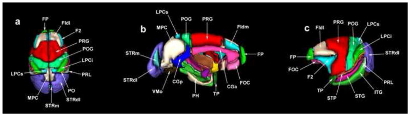
3-D surface renderings of the cortical parcellation units (PUs) used in the present parcellation system in the monkey. Abbreviations: CGa: anterior cingulate gyrus; CGp: posterior cingulate gyrus; F1dl: dorsolateral superior frontal gyrus; F1dm: dorsomedial superior frontal gyrus; F2: inferior frontal gyrus; FOC: frontoorbital cortex; FP: frontal pole; ITG: inferior temporal gyrus; LPCi: inferior part of the lateral parietal cortex; LPCs: superior part of the lateral parietal cortex; MPC: medial parietal cortex; PH: parahippocampal gyrus; POG: postcentral gyrus; PRG: precentral gyrus; PRL: prelunate gyrus; STG: superior temporal gyrus; STP: supratemporal plane; STRdl: dorsolateral striate cortex; STRm: medial striate cortex; TP: temporal pole; VMO: medial occipital cortex.

C) Diffusion Imaging

C₁ Diffusion Tensor MRI Currently, our research group has utilized three different strategies to analyze DT-MRI data: a) ROI-based individual analysis, b) tractography, and c) voxel-based inter-group difference fractional anisotropy (FA) map analysis.

a) ROI-based Segementation

This analysis consists of tensor solution analysis, color-coding and generation of principal eigenvector maps (PEMs), and segmentation of individual fiber tracts.

The tensor solution analysis is based on measurements of diffusion properties for each individual subject. A diffusion image is “built” as follows. The acquisition of the DT-MRI requires the acquisition of six directionally weighted samples of the effect of the diffusion process relative to the axes of the imaging system. In addition, the attenuation of MR signal in the presence of gradients in each of these directions is calculated relative to a baseline (an image acquired with no diffusion encoding. Therefore, a minimum of seven total acquisitions are required (six directions and one baseline). Based on these seven measurements the diffusion tensor (D) is computed (19) and then the directionality of diffusion is assessed by an eigen decomposition of the diffusion tensor.

Color-coding and generation of PEMs

To visualize the direction and location of fiber bundles, a color is assigned for each voxel location by using the primary eigenvector (corresponding to the largest eigenvalue) of D. At each voxel, the absolute values of the x, y, and z components are used as the red, green, and blue color values, respectively, such that a red voxel in the image means the vector points left-right (or right-left), green means the vector points anterior-posterior (or posterior-anterior), and blue means that the vector points superior-inferior (or inferior-superior). For instance, if the primary eigenvector of the diffusion tensor for a given voxel is nearly parallel to the x-axis, then the x value of the vector will be large and the color will be pure red. The color of oblique vectors will be a mixture of red, green and blue depending on the magnitudes of the vector components. This color-coding scheme is shown in Figure 2 with the appropriate color painted onto a sphere. The principal eigenvector map (PEM) is the result of color-coding a tensor image. The PEM can incorporate information about the magnitude of diffusion anisotrophy by making the intensity of the color proportional to an anisotrophy metric. This emphasizes the stems (i.e., the compact portions of the fiber tracts) by diminishing the brightness of everything else. Here “anisotropy” is either fractional or lattice anisotropy (20, 21, 39, 58, 89). Since the particular sensitivities of these anisotropy measures differ, there is no a priori reason to limit the type of anisotropy to the observation of any particular structure (90). By definition these resulting maps, i.e., the PEMs are in exact registration with the diffusion-weighted acquisition.

Figure 2.

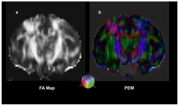
In this figure are shown three steps of the methodology used for the creation of a diffusion image as explained in detail in the text. The tensor representation can be visualized in various ways. For instance: a) a fractional anisotropy (FA) map shows bright regions of high anisotropy; b) a primary eigenvector map (PEM) demonstrates the orientation of the major axis of the diffusion ellipse in 3-D space which can be modulated by anisotropy such as fractional or lattice anisotropy to emphasize the stems of the fiber tracts by decreasing the brightness of surrounding (less anisotropic) voxels. Both a) and b) are in registration as they are the same image processed differently. The colored sphere in the lower center shows the color-coding RGB scheme that has been adopted. Red indicates left-right (or right-left), green indicates anterior-posterior (or posterior-anterior), and blue indicates superior-inferior (or inferior-superior) orientation.

For the segmentation of individual fiber tracts we use the color-coded PEMs on which we identify, select and label the voxels pertaining to each individual fiber bundle on each coronal slice as determined by relative location, orientation, and anatomic specification. We complete the segmentation procedure by progressing in the rostrocaudal dimension through all coronal sections relevant for a specific bundle. Thus we identify, select and label the voxels that belong to a specific fiber tract comprehensively. In practical terms this is reliably done only for the “stems” of the fiber bundles where the fibers run compact from origin to termination (20, 58). This approach has been named “color-map approach” (53); it is documented in detail in previous publications of ours (20, 55) and has been used in Application A2a (i.e., in “DT-MRI: ROI-based Individual Analysis”) as well. This procedure generates specific regions of interest (ROIs) in each individual subject. For each region of interest (ROI), the size (number of voxels and volume), mean, and standard deviation of fractional anisotropy (FA) are calculated. These diffusion parameters (size, and anisotropy) characterizing specific brain ROIs can be eventually correlated with values derived from the other MRI modalities. For all analyses described above there can be used available tools such as TK-Medit and SVV (surface and volume visualizer). SVV allows 3-D reconstructions of fiber tracts based on the relevant voxels selected manually on each coronal slice using TK-Medit.

b) Tractography

Diffusion tensor tractography (DTT) allows reconstruction of 3-D representations of fiber tracts using the fiber assignment by continuous tracking (FACT) algorithm (53, 91). In brief, using FACT (53) fiber tracking is done based on a process of following the flow field of the principal eigenvectors. Tracking is initiated from the center of a voxel and proceeds according to the vector direction. At the point where the track leaves the voxel and enters the next, its direction is changed to that of the neighbor. The continuity of the fiber trajectory is affected by the occurrence of sudden transitions in the fiber orientation and local anisotropy (53). The tractographic method used for the cingulum bundle (CB) is shown in Figure 3. In 3a, the color fractional anisotropy (FA) map or principal eigenvector map (PEM) is shown in a coronal section. The gray scale map of the identical coronal section is used as background in 3b, c. In 3b, one region of interest (ROI) for the left hemisphere was selected as seed location to initiate the fiber tracking process. This ROI was strategically placed on the stem of CB based on the FA color map. It should be pointed out that anatomically driven selection of seed locations and a priori anatomical knowledge of the tracts are necessary for the successful delineation and interpretation of a fiber pathway using tractography. The rostral portion of CB (3c) in the left hemisphere is shown from the fiber tracking process of neighboring voxels that had a primary diffusion orientation close (as determined by an angular threshold) to the orientation of the seed voxel. The color gives the orientation of the eigenvector as shown in the colored sphere. The CB (3d) is contrasted against a background consisting of a FA map of a mid-sagittal plane. Gray scale maps of a coronal plane are added for reference. Similarly, tractography can be performed using HARDI datasets.

Figure 3.

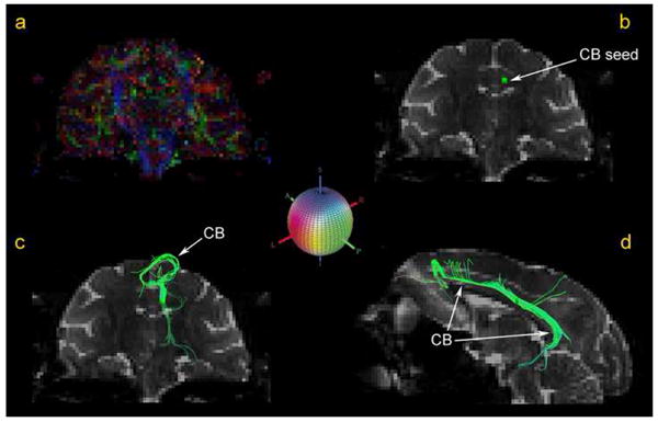
The cingulum bundle (CB) is shown in figure 3a-d as traced using DT-MRI-based tractography. In 3a, the color fractional anisotropy (FA) map or principal eigenvector map (PEM) is shown in a coronal section. The gray scale map of the identical coronal section is used as background in 3b, c. In 3b, one region of interest (ROI) for the left hemisphere was selected as seed location to initiate the fiber tracking process. This ROI was strategically placed on the stem of CB based on the FA color map. The rostral portion of CB (3c) in the left hemisphere is shown as resulted from the fiber tracking process. The color gives the orientation of the eigenvector as shown in the colored sphere, which shows the color-coding RGB scheme that has been adopted. Red indicates left-right (or right-left), green indicates anterior-posterior (or posterior-anterior), and blue indicates superior-inferior (or inferior-superior) orientation. The longitudinal extent of the CB is shown in d) contrasted against a background consisting of a FA map of a mid-sagittal plane.

c) Voxel-based inter-group FA map analysis

3-D volumetric comparisons of FA maps

This FA analysis employs whole brain volumetric techniques. FA maps are first smoothed using a 4mm 3-D Gaussian smoothing kernel. This smoothing provides a more reliable estimate of FA at each point. To register the FA datasets, each participant's smoothed FA map is spatially aligned such as that their AC-PC line is horizontal, the mid-sagittal plane is vertical and the mid-commissural points are aligned. Next, to create group FA maps, we average the datasets of all subjects within each age group. A t-test is then performed at each voxel to determine inter-group differences in FA. Next, we threshold the maps at a level adjusted for multiple comparisons. To visualize the data within an anatomical context, the inter-group differences are displayed onto an average anatomical dataset created from the anatomical datasets of all subjects participating in the study. For this analysis, software is used in the FreeSurfer environment or in FSL.

C₂ High angular resolution diffusion imaging (HARDI) QBI reconstructs the diffusion orientation distribution function (ODF) (u) from the diffusion signal by using the Funk-Radon transform (61). The diffusion ODF describes the probability for a spin to displace in a cylindrical element around the director u. The diffusion ODF is defined as the radial projection of the diffusion probability density function (PDF), $\psi (u)=\frac{1}{z}{\int }_0^{\infty }drP(r\mathbf{\text{u}})$ where P(r) is the PDF and r is the relative spin diffusion vector (61). Visualizations can be generated using TrackVis (92). Recently, a new reconstruction scheme for QBI, termed multiple wavevector fusion (MWF), has been developed. This substantially boosts the sampling efficiency and signal-to-noise of QBI (66). The MWF reconstruction operates by nonlinearly fusing the diffusion signal from separate DTI and QBI acquisitions (66). In addition, an intravoxel peak connectivity metric (IPCM) has been developed, which calculates the peak connectivity between an ODF and its neighboring voxels.

D) Magnetization Transfer MRI (MT-MRI)

Voxel-based inter-group difference MTR map analysis: 3-D volumetric comparisons of MTR maps: To register the MTR datasets, each participant's MTR map is spatially aligned such that their AC-PC line is horizontal, the mid-sagittal plane is vertical and the mid-commissural points are aligned. We compute the MTR for each individual for all voxels of its dataset (67, 93, 94). Then within each group we compute the average and standard deviation of each voxel and we create the group map. Then we create the inter-group difference map by computing a t-test on a voxel-by-voxel basis. We then visualize the data thresholding on the maps and adjust for multiple comparisons. Finally, we display them onto an average anatomic brain, which is created from the T1 morphometric datasets of the subjects participating in the study. For the analyses described above we have used in-house tools in the domain of the FreeSurfer system (95).

E) Integrated MR neuro-exam

A number of recently developed magnetic resonance (MR) techniques such as structural T1-weighted MRI and DT-MRI allow for measurement of parameters relevant to the neurobiological mechanisms of cognitive and behavioral phenomena. The comprehensive integration of such multidimensional datasets has laid the groundwork for enabling measures of brain cortical and subcortical gray structures and fiber tracts. Multimodal data must be integrated into a common coordinate space to permit unified representation of the brain and to compute differences between individuals and groups, resulting in a host of measures that represent a quantitative dimension vector and can be used to elucidate the structural underpinnings of the structural, functional, behavioral and clinical dimension vector statistically. For instance, the relative contributions of each of these imaging modalities can be assessed for any developmental, aging or degenerative process using principal component analysis. Consequently, the cognitive and emotional networks in normality and their alterations in disease become the targets for intervention and for developing effective treatments that may rectify the disease process and lead to healing. The non-invasive nature of MRI allows repeated experiments on an individual subject, either during the course of one examination period or on multiple occasions. These data must be registered accurately, in both space and time, and interpreted to isolate physiological phenomena of interest from extraneous sources. Three-dimensional, high-resolution, anatomic MRI images will serve as the basis for interrelating this information.

It is important that computational models investigating variability of structure be able to integrate these multiple data representations. This will lead to an optimized, temporally efficient MRI neuro-exam that captures the salient features of the structural, metabolic and functional states as they change over time. Monitoring these manifestations could elucidate the neurobiological underpinnings of normal brain development and aging, as well as the end points of etiology, natural history and therapeutic intervention in disease states (24).

E) Correlations of Imaging Studies with Behavior

The monkeys used in our study were repeatedly tested over a period spanning approximately nine months with a battery of behavioral tests assessing learning, attention, executive function and recognition memory (6, 96). In our analysis, the monkeys were stratified based on age in two groups, i.e., young (less or equal to 15 years of age) and old (more than 15 years of age) (6). Data from the neuroimaging studies were compared with age-related changes in cognitive function in the following way. First, specific regions of interest (ROIs) including specific frontal and temporal fiber tracts (such as the superior longitudinal fascicle II, the cingulum bundle and the anterior part of the corpus callosum as identified in the DT-MRI) are selected and measures of their average FA are determined in both the right and left hemispheres in each subject. These FA measures are then summed across hemispheres to produce a bilateral mean FA value. Those tract-specific measures of fractional anisotropy, within the aged group, are then correlated with two different sets of behavioral measures of cognitive function such as executive function and recognition memory (6). Results of this specific study are summarized later on, under Application A4 (i.e., “Structural-behavioral correlations”). Similarly, behavioral measures can be correlated with other structural measures such as volume.

Applications in the Aging Monkey Brain Using Structural MRI

In what follows, we surveyed sample applications relevant to the aging monkey brain using T1-MRI based morphometric analysis (A1), diffusion imaging (A2), magnetization transfer MRI (A3) and structural-behavioral correlations (A4).

A1. Morphometric Analysis application

The results presented here are related to segmentation (Figure 4) (global cortical and subcortical) and detailed cortical parcellation (Figures 4 and 5) on monkey brains. The specific information regardingof the morphometric imaging protocol used for this study as well as preliminary results related to the completed segmentation of 19 brains are given in Table 1 and the cortical parcellation of one brain is given in Table 2.

Table 1.

Results of segmentation in 19 rhesus monkey brains. The volumes of the different structures are expressed in cm³.

Structure		Young (N=12)	Old (N=7)
Whole Brain*		95.7 +/- 12.9	91.3 +/- 11.7
Total Cerebrum		82.8 +/- 11.5	78.6 +/- 10.5
Neocortical Gray Matter (Cortex)		46.3 +/- 6.8	40.5 +/- 4.7
White Matter		26.6 +/- 4.5	28.5 +/- 5.0
Hippocampus		1.0 +/- 0.1	1.0 +/- 0.1
Amygdala		0.5 +/- 0.1	0.5 +/- 0.1
Lateral Ventricle		0.8 +/- 0.2	0.9 +/- 0.4
Basal Ganglia
Caudate		1.0 +/- 0.2	0.9 +/- 0.2
Nucleus Accumbens		0.2 +/- 0.1	0.2 +/- 0.0
Putamen		1.8 +/- 0.3	1.6 +/- 0.3
Pallidum		0.7 +/- 0.1	0.8 +/- 0.2
Diencephalon		3.9 +/- 0.5	3.7 +/- 0.5
Thalamus		1.8 +/- 0.2	1.7 +/- 0.3
Ventral Diencephalon**		2.1 +/- 0.3	2.0 +/- 0.3

Table 2.

Results of cortical parcellation in one rhesus monkey cerebrum. Volumes (cm³) of frontal, temporal, parietal and occipital neocortical parcellation units in a monkey brain (N=1).

Region		Right Volume (cm3)	Left Volume (cm3)	Total Volume (cm3)
Cerebrum		37.13	37.45	74.58
Frontal Lobe		12.77	12.85	25.62
Cortex		6.60	6.64	13.24
	FP	0.29	0.37	0.66
	F1dl	0.87	0.78	1.65
	F1dm	0.30	0.27	0.57
	F2	0.57	0.66	1.22
	PRG	2.68	2.69	5.37
	COa	0.18	0.19	0.37
	FOC	0.92	0.85	1.77
	CGa	0.71	0.76	1.46
	SC	0.09	0.09	0.18
Temporal Lobe		9.10	8.93	18.03
Cortex		6.05	5.94	11.99
	TP	0.41	0.38	0.79
	STG	1.34	1.30	2.64
	ITG	2.61	2.57	5.18
	STP	0.61	0.63	1.24
	PH	0.65	0.61	1.26
	INS	0.43	0.45	0.88
Parietal Lobe		7.05	7.10	14.15
Cortex		4.03	4.13	8.16
	COp	0.19	0.19	0.38
	CGp	0.47	0.55	1.02
	MPC	1.24	1.29	2.53
	POG	1.16	1.17	2.33
	LPCs	0.27	0.27	0.54
	LPCi	0.70	0.66	1.36
Occipital Lobe		9.06	9.45	18.51
Cortex		5.60	5.85	11.45
	PRL	0.85	0.88	1.73
	STRdl	3.25	3.46	6.71
	STRm	0.47	0.48	0.95
	VMO	1.03	1.03	2.06

Abbreviations: BSF=basal forebrain, COa=anterior central operculum, CGa=anterior cingulate gyrus cortex, F1dl=superior frontal gyrus cortex (dorsolateral), F1dm=superior frontal gyrus cortex (dorsomedial), F2=inferior frontal gyrus cortex, FOC=frontoorbital cortex, FP=frontopolar cortex, INS=insular cortex, PH=parahippocampal gyrus cortex, SC=subcallosal cortex, STP=supratemporal cortex, T1=superior temporal gyrus cortex, T3=inferior temporal gyrus cortex, TP=temporopolar cortex.

Morphometric Imaging protocol Preliminary results were obtained using 1.5-TeslaSiemens Sonata magnet at the MGH-NMR Center located in the MGH-East complex at the Charlestown Navy Yard, Charlestown, Massachusetts. This involved MP-RAGE volume acquisitions, with 1.0 mm thick sagittal slices for a total of 128 effective slices, 0 gap (increasing slice thickness if necessary to cover complete brain), in plane resolution .8 × .8 mm²; TR=2.730 milliseconds (ms), TE=2.8 ms (minimum), TI=300 ms, Flip Angle=7 degrees, matrix=256 × 256, bandwidth=190 Hz/pixel, NEX=4 to obtain high signal to noise ratio. The acquisition time is approximately 40 minutes.

Segmentation and Cortical parcellation The anatomic analysis is designed in a hierarchical fashion as diagrammed in Figure 8. The first step is a general segmentation system, which divides the brain into large regional units of analysis, including cerebrum, cerebellum, ventricles and brainstem, with a potential further subdivision of the cerebellum (80, 81, 97). General segmentation then subdivides the cerebrum into cerebral cortex, central white matter, hippocampus, amygdala, lateral ventricles, caudate, putamen, globus pallidus, nucleus accumbens septi and thalamus (Figure 4). The next step is subdivision of cerebral cortex, subcortical gray matter and central white matter (81). This fine-grain parcellation of the cerebrum is referenced to a set of neuroanatomic landmarks, which are robustly visible on MRI scans. These are principally sulci, or intersections of sulci with the consequence that the neocortical parcellation units correspond principally to complete or parts of the canonical set of gyri of the normal human brain (78, 88). Gyral topography can be adequately referenced to underlying cytoarchitectonic subdivisions and thereby to specific neural systems components (98-100). Thus this system recognizes the classic lobar subdivisions (frontal, temporal, parietal, occipital, limbic) or gyri and it can approximate the hierarchical systems organization as has been described by (101). Overall, twenty-five regions of interest (i.e., parcellation units or PUs) were parcellated. Eight PUs resided within the frontal lobe and included frontal pole (FP), superior frontal gyrus (F1) (including both, the dorsolateral F1 or F1dl and the dorsomedial F1 or F1dm), inferior frontal gyrus (F2), frontoorbital cortex (FOC), precentral gyrus (PRG), anterior part of the central operculum (COa), anterior cingulate gyrus (CGa) and subcallosal cortex (SC). The temporal lobe was composed of six PUs including the temporal pole (TP), supratemporal plane (STP), superior temporal gyrus (STG), inferior temporal gyrus (ITG), parahippocampal gyrus (PH) and the insula (INS). The parietal lobe included seven PUs, which were the postcentral gyrus (POG), posterior part of the central operculum (COp), superior part of the lateral parietal cortex (LPCs), inferior part of the lateral parietal cortex (LPCi), medial parietal cortex (MPC and posterior cingulate gyrus (CGp). Finally, the occipital lobe was subdivided into four PUs, which included the prelunate gyrus (PRL), dorsolateral striate cortex (STRdl), medial striate cortex (STRm), dorsal part of the medial occipital cortex (DMO) and ventral part of the medial occipital cortex (VMO).

Figure 8.

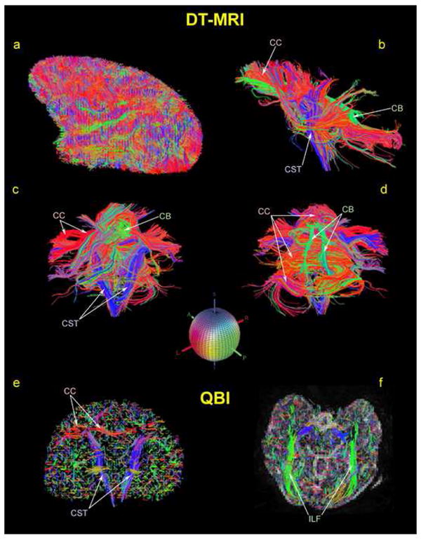
An array of reconstructed fiber tracts based on the DT-MRI data of a rhesus monkey using the TrackVis software package is shown. Specifically, the corpus callosum (CC) in red, the corticospinal tract (CST) in blue and the cingulum bundle (CB) in green are illustrated. The colored sphere shows the color-coding RGB scheme that has been adopted. Red indicates left-right (or right-left), green indicates anterior-posterior (or posterior-anterior), and blue indicates superior-inferior (or inferior-superior) orientation.

The images shown in Figure 5 were produced by an in-house software system (named “surface and volume visualizer” or SVV) that allowed us to visualize surfaces reconstructed from the segmentation and cortical parcellation data.

A2. Diffusion Imaging

We have analyzed ten brain datasets of healthy rhesus monkeys using DT-MRI (6). These ten monkeys pertained to two different age groups; specifically five monkeys were young (age 5 to 10) and five were old (20 years of age and older).

DT-MRI The preliminary results were obtained using a 1.5-Tesla Siemens Sonata scanner. We sampled the diffusion tensor, D, using a seven-shot T2-echo-planar imaging (EPI) technique with the following parameters: TR = 5200 ms, TE = 60 ms, averages = 96 (4 measurements of 24 averages each), number of slices = 40 to cover the entire brain, FOV = 166.4, data matrix = 128 × 128, in-plane voxel resolution = 1.3 × 1.3 mm², slice orientation was in the coronal plane, slice thickness = 2 mm, skip 1 mm, bandwidth = 1220 Hz/pixel, diffusion sensitivity: b = 600 s/mm², with approximate SNR = 100 and imaging time of approximately 75 minutes. Diffusion tensor images are generated by fitting a tensor model to the registered images containing the directional information.

Several observations were made using the acquired DT-MRI datasets based on three different types of analyses as follows.

a) ROI-based Individual Analysis

In this preliminary analysis a specific region of interest (ROI), the cingulum bundle (CB) was identified, segmented and measured on each individual monkey brain dataset. For the CB ROI, the size (number of voxels and volume), and the fractional anisotropy (FA) were measured. In Figure 6 the result of a manual segmentation of the CB on a single coronal slice is shown. By progressing in the rostrocaudal dimension throughout the entire trajectory of this bundle we segmented its stem comprehensively on a coronal slice-by-slice fashion (55). This manual procedure has been named segmentation “color-based approach.” The results of this analysis are shown in Table 3.

Figure 6.

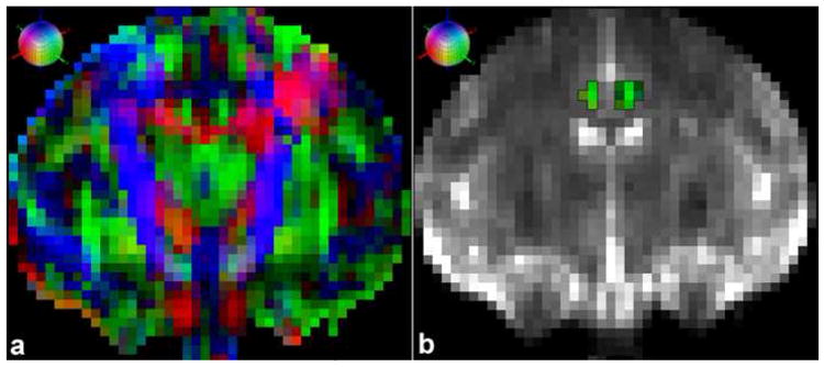
(a) Coronal DT-MRI principal eigenvector map (PEM) of a rhesus macaque brain. (b) Coronal T2-MR image with the color-coded (green voxels) segmented cingulum bundle (CB) registered. Scanning was done using the 1.5-Tesla Siemens Sonata system. Each voxel in the image was assigned a color based on the orientation of the largest eigenvalue of the diffusion tensor. A red voxel in the image means the vector points left-right (or right-left), green means the vector points anterior-posterior (or posterior-anterior), and blue means that the vector points superior-inferior (or inferior-superior). The colored sphere shows the adopted RGB color-coding scheme.

Table 3.

Diffusion Tensor Imaging statistics of the cingulum bundle (CB) in monkeys. SEM is standard error of the mean.

Group	Animal	Fractional Anisotropy	Lattice Anisotropy	Number of Voxels	Volume (cm3)
Young (N=5)	1	0.12 (0.10)	0.12 (0.05)	103.00	0.35
	2	0.11 (0.09)	0.11 (0.05)	146.00	0.49
	3	0.18 (0.12)	0.18 (0.09)	108.00	0.37
	4	0.18 (0.10)	0.18 (0.07)	180.00	0.61
	5	0.17 (0.11)	0.17 (0.08)	180.00	0.61
	Mean	0.15	0.15	143.40	0.48
	SEM	0.01	0.01	7.46	0.03
Old (N=5)	1	0.16 (0.04)	0.07 (0.03)	27.00	0.09
	2	0.18 (0.11)	0.18 (0.08)	154.00	0.52
	3	0.13 (0.11)	0.13 (0.06)	146.00	0.49
	4	0.17 (0.08)	0.17 (0.06)	159.00	0.54
	5	0.11 (0.08)	0.11 (0.05)	87.00	0.29
	Mean	0.15	0.13	114.60	0.39
	SEM	0.01	0.01	11.38	0.04
	Total Mean	0.15	0.15	124.85	0.42
	Total SEM	0.00	0.00	3.27	0.01

These data are consistent with the possibility that CB volume decreases, beginning in middle age. To test this, more animals are needed. In addition, the utilization of a scanning protocol that allows the acquisition of smaller voxels would increase the accuracy for identification and segmentation of individual fiber stems.

Preliminary results from one monkey dataset scanned on a 3-Tesla Siemens Allegra system are shown in Figure 7. Higher magnetic fields than 1.5 Tesla allow the acquisition of smaller isotrophic voxels for a similar signal-to-noise ratio (SNR).

Fig 7.

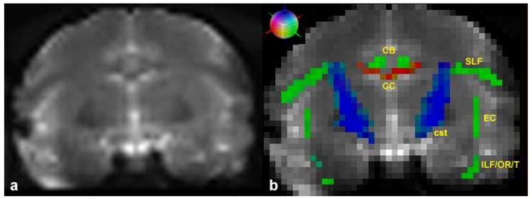
(a) Coronal T2-EPI image of a rhesus macaque brain. (b) Segmented color-coded fiber tracts registered on the identical coronal slice. Scanning was done using the 3-Tesla Siemens Allegra system. Red color-coding corresponds to left-right (or right-left), green to anterior-posterior (or posterior-anterior), and blue to superior-inferior (or inferior-superior). Abbreviations: CB=cingulum bundle (green), CC=corpus callosum (red), CST=corticospinal tract (blue), EC=extreme capsule (green), ILF/OR/T=inferior longitudinal fasciculus/optic radiation/tapetum complex (green), SLF=superior longitudinal fasciculus (green). Besides the CC and CB that are located in the medial part of the cerebrum, the rest of the bundles shown in this figure (i.e., SLF, EC, ILF/OR/T, and cst) course more laterally and their counterparts (not labeled) are mirrored on the opposite hemisphere. The colored sphere indicates the adopted RGB color-coding scheme. Red indicates left-right (or right-left), green indicates anterior-posterior (or posterior-anterior), and blue indicates superior-inferior (or inferior-superior) orientation.

b) Tractography

We show an array of reconstructed fiber tracts based on the DT-MRI and HARDI (QBI) data of a rhesus monkey using the TrackVis software package. The corpus callosum, corticospinal tract and cingulum are depicted in Figure 8.

c) Voxel-based inter-group difference FA map analysis: Mapping FA data

Once the FA datasets of the thirteen monkeys participating in this preliminary study were registered, the FA map for each individual was created and then within each group we computed the average and standard deviation of each voxel and we created the average group map. Thus three group average FA maps were created, i.e., one for each age group (young, middle-aged, and old). Then we created the three different (young vs. old, young vs. middle-aged, and middle-aged vs. old) inter-group maps by computing a t-test on a voxel-by-voxel basis and we thresholded the maps. These preliminary results were uncorrected for multiple comparisons due to the fact that the number of subjects participating in the study was low. The inter-group difference FA maps were displayed onto an average anatomic brain, which was created from the thirteen T1 morphometric datasets of the subjects participating in this preliminary study.

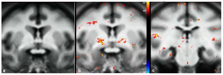
As shown in Figure 9, in which an inter-group difference of FA maps for the young group (N=5) vs. the old group (N=5) is displayed, FA is sensitive to age related changes in the white matter. The results, although preliminary, suggest that there could be specific fiber tracts that are selectively vulnerable to these changes. These fiber tracts are mainly association and commissural fibers interconnecting the associative cortical areas of the different lobes. In particular, the superior and inferior longitudinal fascicles were involved as well as the cingulum bundle and the corpus callosum. These preliminary findings suggest that DT-MRI could be a promising avenue to investigate age related fiber tract changes in the monkey.

Figure 9.

Inter-group difference FA maps in the monkey. A representative coronal slice of the average anatomical brain at the level of the callosal genu is shown in (a). The FA statistical map of inter-group difference (young vs. old) for this level is displayed in (b) onto the average anatomical image showing bilateral statistically significant (p<.05) differences in the superior longitudinal fasciculus bilaterally and the callosal genu.

A3. Magnetization Transfer MRI (MT-MRI)

Thirteen brain datasets of healthy rhesus monkeys were scanned and analyzed. Of these monkeys, seven were young (age 5 to 10 15 to 19) and three were old (20 years of age and older). All of them were scanned for MT-MRI and then two different types of analyses were performed: a) ROI-based individual analysis, and b) voxel-based inter-group difference magnetization transfer ratio (MTR) map analysis. The MT analysis includes intra-subject registration for the calculation of the individual MTR maps, as well as inter-subject registration to perform the inter-group voxel-based analysis.

Imaging The preliminary results were obtained using the 1.5T Siemens Sonata scanner. Voxel-based inter-group difference MTRmap analysis: To map MT ratios (MTRs) all MT-MRI datasets were registered. Then we created the MTR map for each individual and subsequently within each group we computed the average group map. We then created the inter-group MTR difference maps. The inter-group difference MTR maps were displayed onto an average anatomic brain, which was created from the thirteen T1 morphometric datasets of the subjects participating in this preliminary study.

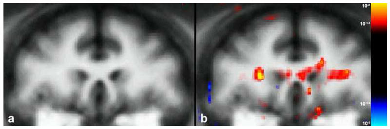
As shown in these figures the magnetization transfer contrast is sensitive to age related changes in the white matter and the results are regionally selective yet bilateral suggesting that there could be specific white matter pathways (rather than a more diffuse process) that are selectively vulnerable to these changes (Figure 10). These preliminary results suggest that myelin changes may occur in the white matter of the older monkeys and that myelin defects may be higher in the older group. They also suggest that magnetization transfer could be a useful way to quantify and localize age related alterations in myelination.

Figure 10.

Results of inter-group MTR difference statistical map analysis between young and old monkeys shown in two representative coronal slices. In (a) a representative coronal slice of the average anatomical brain at the level of the anterior commissure is shown. b) MTR statistical maps were displayed onto the average anatomical image showing bilateral statistically significant (p<.001) differences in the anterior commissure, superior longitudinal fasciculus and cingulum bundle. At a more posterior coronal level (c) these differences are pronounced at the right inferior longitudinal fasciculus and the left cingulum bundle.

A4. Structural-behavioral correlations

In this example application, we report a published result of our group (6), in which we correlated FA measures of specific fiber tracts connecting the prefrontal cortex such as the superior longitudinal fascicle II, the cingulum bundle and the anterior part of the corpus callosum with behavioral measures for cognitive function. Interestingly, these three prefrontal fiber tracts showed correlations of lower FA values associated with poorer performance in a task of executive function, i.e., the Conceptual Set Shifting Task (CSST), a monkey version of the human Wisconsin Card Sort Test (6) (Figure 11).

Figure 11.

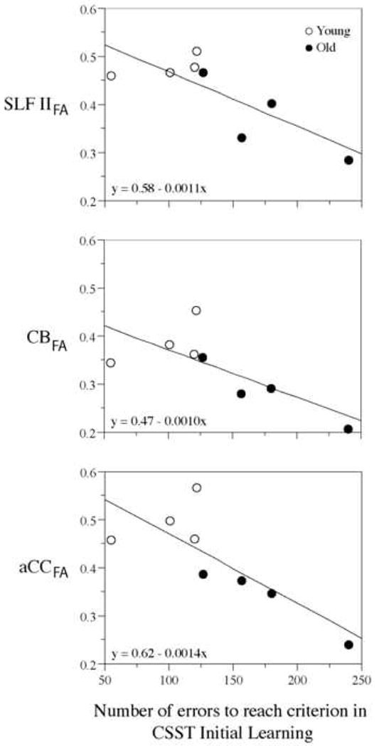
Scatterplots showing the correlations between FA maps of bilateral regions of interest and the number of errors to reach criterion performance in the initial learning phase of the Cognitive Set Shifting Task (CSST). Linear regression lines are shown, as well as fitting equations. The plot symbols are distinct for the young and old monkey groups for display purposes only. These plots show a correlation of lower FA values in CB, SLF II and aCC associated with poorer performance. In addition, there is shown a separation between young and old monkeys indicating that this could be related to an age effect (6). Abbreviations: CB: cingulum bundle; SLF II: superior longitudinal fascicle II; aCC: anterior corpus callosum; CSST: Cognitive Set Shifting Task.

Conclusion

This review has addressed quantitative neuroimaging studies of the aging monkey brain, the integration of different imaging modalities in brain structure analysis, and the correlation of behaviors with brain structure. It elaborates on the classes of information that are readily available in the MR image and methods for extracting quantitative results, and presents sample applications of these types of techniques to the monkey brain. These applications emphasize tissue and anatomically based contrasts regarding the nature of structural change, and the repercussions of brain changes with specific behaviors as a function of aging. The results underscore our capability to study changes in the monkey brain structures - quantitatively and in vivo – during the aging process and associate them with changes in specific behaviors and cognitive decline.

References

- 1.Peters A, Morrison JH, Rosene DL, Hyman BT. Cereb Cortex. 1998;8:295–300. doi: 10.1093/cercor/8.4.295. [DOI] [PubMed] [Google Scholar]
- 2.Peters A, Rosene DL. J Comp Neurol. 2003;462:139–43. doi: 10.1002/cne.10715. [DOI] [PubMed] [Google Scholar]
- 3.Peters A, Rosene DL, Moss MB, Kemper TL, Abraham CR, Tigges J, Albert MS. J Neuropathol Exp Neurol. 1996;55:861–74. doi: 10.1097/00005072-199608000-00001. [DOI] [PubMed] [Google Scholar]
- 4.Sandell JH, Peters A. J Comp Neurol. 2003;466:14–30. doi: 10.1002/cne.10859. [DOI] [PubMed] [Google Scholar]
- 5.Guttmann CR, Jolesz FA, Kikinis R, Killiany RJ, Moss MB, Sandor T, Albert MS. Neurology. 1998;50:972–8. doi: 10.1212/wnl.50.4.972. [DOI] [PubMed] [Google Scholar]
- 6.Makris N, Papadimitriou GM, van der Kouwe A, Kennedy DN, Hodge SM, Dale AM, Benner T, Wald LL, Wu O, Tuch DS, Caviness VS, Moore TL, Killiany RJ, Moss MB, Rosene DL. Neurobiol Aging. 2007;28:1556–67. doi: 10.1016/j.neurobiolaging.2006.07.005. [DOI] [PubMed] [Google Scholar]
- 7.Persson J, Nyberg L, Lind J, Larsson A, Nilsson LG, Ingvar M, Buckner RL. Cereb Cortex. 2006;16:907–15. doi: 10.1093/cercor/bhj036. [DOI] [PubMed] [Google Scholar]
- 8.Walhovd KB, Fjell AM, Reinvang I, Lundervold A, Dale AM, Eilertsen DE, Quinn BT, Salat D, Makris N, Fischl B. Neurobiol Aging. 2005;26:1261–70. doi: 10.1016/j.neurobiolaging.2005.05.020. discussion 75-8. [DOI] [PubMed] [Google Scholar]
- 9.Gomez-Isla T, Price JL, McKeel DW, Jr, Morris JC, Growdon JH, Hyman BT. J Neurosci. 1996;16:4491–500. doi: 10.1523/JNEUROSCI.16-14-04491.1996. [DOI] [PMC free article] [PubMed] [Google Scholar]
- 10.Haug T. In: Senile Dementia of the Alzheimer's Type. Traber J, Gispen WH, editors. Springer-Verlag; Berlin: 1985. pp. 150–63. [Google Scholar]
- 11.Pakkenberg B, Gundersen HJ. J Comp Neurol. 1997;384:312–20. [PubMed] [Google Scholar]
- 12.Marner L, Nyengaard JR, Tang Y, Pakkenberg B. J Comp Neurol. 2003;462:144–52. doi: 10.1002/cne.10714. [DOI] [PubMed] [Google Scholar]
- 13.Haacke EM. Magnetic resonance imaging: physical principles and sequence design. J. Wiley & Sons; New York: 1999. [Google Scholar]
- 14.Hinshaw WS, Lent AH. Proc IEEE. 1983;71 [Google Scholar]
- 15.Caputo GR, Kondo C, Higgins CB. Am J Card Imaging. 1993;7:233–42. [PubMed] [Google Scholar]
- 16.Aksoy FG, Lev MH. Semin Ultrasound CT MR. 2000;21:462–77. doi: 10.1016/s0887-2171(00)90038-6. [DOI] [PubMed] [Google Scholar]
- 17.Rosen BR, Belliveau JW, Aronen HJ, Kennedy D, Buchbinder BR, Fischman A, Gruber M, Glas J, Weisskoff RM, Cohen MS, et al. Magn Reson Med. 1991;22:293–9. doi: 10.1002/mrm.1910220227. discussion 300-3. [DOI] [PubMed] [Google Scholar]
- 18.Sudikoff S, Banasiak K. Curr Opin Pediatr. 1998;10:291–8. doi: 10.1097/00008480-199806000-00012. [DOI] [PubMed] [Google Scholar]
- 19.Basser PJ, Mattiello J, LeBihan D. J Magn Reson B. 1994;103:247–54. doi: 10.1006/jmrb.1994.1037. [DOI] [PubMed] [Google Scholar]
- 20.Makris N, Worth AJ, Sorensen AG, Papadimitriou GM, Wu O, Reese TG, Wedeen VJ, Davis TL, Stakes JW, Caviness VS, Kaplan E, Rosen BR, Pandya DN, Kennedy DN. Ann Neurol. 1997;42:951–62. doi: 10.1002/ana.410420617. [DOI] [PubMed] [Google Scholar]
- 21.Pierpaoli C, Basser PJ. Magn Reson Med. 1996;36:893–906. doi: 10.1002/mrm.1910360612. [DOI] [PubMed] [Google Scholar]
- 22.Ogawa S, Tank DW, Menon R, Ellermann JM, Kim SG, Merkle H, Ugurbil K. Proc Natl Acad Sci U S A. 1992;89:5951–5. doi: 10.1073/pnas.89.13.5951. [DOI] [PMC free article] [PubMed] [Google Scholar]
- 23.Guimaraes AR, Baker JR, Jenkins BG, Lee PL, Weisskoff RM, Rosen BR, Gonzalez RG. Magn Reson Med. 1999;41:877–82. doi: 10.1002/(sici)1522-2594(199905)41:5<877::aid-mrm4>3.0.co;2-3. [DOI] [PubMed] [Google Scholar]
- 24.Jenkins BG, Chen YI, Kuestermann E, Makris NM, Nguyen TV, Kraft E, Brownell AL, Rosas HD, Kennedy DN, Rosen BR, Koroshetz WJ, Beal MF. Ann N YAcad Sci. 1999;893:214–42. doi: 10.1111/j.1749-6632.1999.tb07828.x. [DOI] [PubMed] [Google Scholar]
- 25.Ross B, Michaelis T. Magn Reson Q. 1994;10:191–247. [PubMed] [Google Scholar]
- 26.Pineiro R, Pendlebury ST, Smith S, Flitney D, Blamire AM, Styles P, Matthews PM. Stroke. 2000;31:672–9. doi: 10.1161/01.str.31.3.672. [DOI] [PubMed] [Google Scholar]
- 27.Schellinger PD, Fiebach JB, Jansen O, Ringleb PA, Mohr A, Steiner T, Heiland S, Schwab S, Pohlers O, Ryssel H, Orakcioglu B, Sartor K, Hacke W. Ann Neurol. 2001;49:460–9. [PubMed] [Google Scholar]
- 28.Schwamm LH, Koroshetz WJ, Sorensen AG, Wang B, Copen WA, Budzik R, Rordorf G, Buonanno FS, Schaefer PW, Gonzalez RG. Stroke. 1998;29:2268–76. doi: 10.1161/01.str.29.11.2268. [DOI] [PubMed] [Google Scholar]
- 29.Saunders RC, Aigner TG, Frank JA. Exp Brain Res. 1990;81:443–6. doi: 10.1007/BF00228139. [DOI] [PubMed] [Google Scholar]
- 30.Caviness VS, Jr, Filipek PA, Kennedy DN. Brain Dev. 1992;14(Suppl):S80–5. [PubMed] [Google Scholar]
- 31.Bloch F. Physics Review. 1946;70:460. [Google Scholar]
- 32.Chien D, Buxton RB, Kwong KK, Brady TJ, Rosen BR. J Comput Assist Tomogr. 1990;14:514–20. doi: 10.1097/00004728-199007000-00003. [DOI] [PubMed] [Google Scholar]
- 33.Douek P, Turner R, Pekar J, Patronas N, Le Bihan D. J Comput Assist Tomogr. 1991;15:923–9. doi: 10.1097/00004728-199111000-00003. [DOI] [PubMed] [Google Scholar]
- 34.Le Bihan D, Breton E, Lallemand D, Grenier P, Cabanis E. Laval-Jeantet Radiology. 1986;161:401–7. doi: 10.1148/radiology.161.2.3763909. [DOI] [PubMed] [Google Scholar]
- 35.Moseley ME, Cohen Y, Kucharczyk J, Mintorovitch J, Asgari HS, Wendland MF, Tsuruda J, Norman D. Radiology. 1990;176:439–45. doi: 10.1148/radiology.176.2.2367658. [DOI] [PubMed] [Google Scholar]
- 36.Stejskal EO, Tanner JE. Journal of Chemical Physics. 1965;42:288–92. [Google Scholar]
- 37.Torrey H. Phys Rev. 1956;194:563–65. [Google Scholar]
- 38.Turner R, Le Bihan D, Delannoy J, Pekar J. 8th Annual Meeting of the Society of Magnetic Resonance in Medicine; Amsterdam, The Netherlands. 1989. [Google Scholar]
- 39.Basser PJ, Pierpaoli C. J Magn Reson B. 1996;111:209–19. doi: 10.1006/jmrb.1996.0086. [DOI] [PubMed] [Google Scholar]
- 40.Davis TL, Wedeen VJ, Weisskof RM, Rosen BR. 12th Annual Meeting of the Society of Magnetic Resonance in Medicine; New York, NY. 1993. [Google Scholar]
- 41.Filley CM. Neurology. 1998;50:1535–40. doi: 10.1212/wnl.50.6.1535. [DOI] [PubMed] [Google Scholar]
- 42.Pierpaoli CJ. Central Nervous System Spectrums. 2002;7:510–15. [Google Scholar]
- 43.Beaulieu C. NMR Biomed. 2002;15:435–55. doi: 10.1002/nbm.782. [DOI] [PubMed] [Google Scholar]
- 44.Cercignani M, Iannucci G, Rocca MA, Comi G, Horsfield MA, Filippi M. Neurology. 2000;54:1139–44. doi: 10.1212/wnl.54.5.1139. [DOI] [PubMed] [Google Scholar]
- 45.Kubicki M, Westin CF, Maier SE, Mamata H, Frumin M, Ersner-Hershfield H, Kikinis R, Jolesz FA, McCarley R, Shenton ME. Harv Rev Psychiatry. 2002;10:324–36. doi: 10.1080/10673220216231. [DOI] [PMC free article] [PubMed] [Google Scholar]
- 46.Pfefferbaum A, Sullivan EV. Neuroimage. 2002;15:708–18. doi: 10.1006/nimg.2001.1018. [DOI] [PubMed] [Google Scholar]
- 47.Pfefferbaum A, Sullivan EV, Hedehus M, Adalsteinsson E, Lim KO, Moseley M. Alcohol Clin Exp Res. 2000;24:1214–21. [PubMed] [Google Scholar]
- 48.Ellis CM, Simmons A, Jones DK, Bland J, Dawson JM, Horsfield MA, Williams SC, Leigh PN. Neurology. 1999;53:1051–8. doi: 10.1212/wnl.53.5.1051. [DOI] [PubMed] [Google Scholar]
- 49.Moseley M. NMR Biomed. 2002;15:553–60. doi: 10.1002/nbm.785. [DOI] [PubMed] [Google Scholar]
- 50.Nusbaum AO, Tang CY, Buchsbaum MS, Wei TC, Atlas SW. AJNR Am J Neuroradiol. 2001;22:136–42. [PMC free article] [PubMed] [Google Scholar]
- 51.Pfefferbaum A, Sullivan EV, Hedehus M, Lim KO, Adalsteinsson E, Moseley M. Magn Reson Med. 2000;44:259–68. doi: 10.1002/1522-2594(200008)44:2<259::aid-mrm13>3.0.co;2-6. [DOI] [PubMed] [Google Scholar]
- 52.Sullivan EV, Adalsteinsson E, Hedehus M, Ju C, Moseley M, Lim KO, Pfefferbaum A. Neuroreport. 2001;12:99–104. doi: 10.1097/00001756-200101220-00027. [DOI] [PubMed] [Google Scholar]
- 53.Mori S. Central Nervous System Spectrums. 2002;7:529–34. [Google Scholar]
- 54.Pierpaoli C, Jezzard P, Basser PJ, Barnett A, Di Chiro G. Radiology. 1996;201:637–48. doi: 10.1148/radiology.201.3.8939209. [DOI] [PubMed] [Google Scholar]
- 55.Makris N, Pandya DN, Normandin JJ. Central Nervous System Spectrums. 2002;7:522–28. [Google Scholar]
- 56.Conturo TE, Lori NF, Cull TS, Akbudak E, Snyder AZ, Shimony JS, McKinstry RC, Burton H, Raichle ME. Proc Natl Acad Sci U S A. 1999;96:10422–7. doi: 10.1073/pnas.96.18.10422. [DOI] [PMC free article] [PubMed] [Google Scholar]
- 57.Mori S, Crain BJ, Chacko VP, van Zijl PC. Ann Neurol. 1999;45:265–9. doi: 10.1002/1531-8249(199902)45:2<265::aid-ana21>3.0.co;2-3. [DOI] [PubMed] [Google Scholar]
- 58.Makris N, Papadimitriou GM, Worth AJ, Jenkins BG, Garrido L, Sorensen AG, Wedeen V, Tuch DS, Wu O, Cudkowicz ME, Caviness VS, Jr, Rosen B, Kennedy DN. In: Neuropsychopharmacology: The Fifth Generation of Progress. KL Davis, Charney D, Coyle J, Nemeroff C., editors. Lippincott, Williams, and Wilkins; New York: 2002. pp. 357–71. [Google Scholar]
- 59.Davis TL, Tuch DS. Central Nervous System Spectrums. 2002;7:505–09. [Google Scholar]
- 60.Tuch DS, Reese TG, Wiegell MR, Makris N, Belliveau JW, Wedeen VJ. Magn Reson Med. 2002;48:577–82. doi: 10.1002/mrm.10268. [DOI] [PubMed] [Google Scholar]
- 61.Tuch DS. Magn Reson Med. 2004;52:1358–72. doi: 10.1002/mrm.20279. [DOI] [PubMed] [Google Scholar]
- 62.Tuch DS, Reese TG, Wiegell MR, Wedeen VJ. Neuron. 2003;40:885–95. doi: 10.1016/s0896-6273(03)00758-x. [DOI] [PubMed] [Google Scholar]
- 63.Tuch DS, Wisco JJ, Khachaturian MH, Ekstrom LB, Kotter R, Vanduffel W. Philos Trans R Soc Lond B Biol Sci. 2005;360:869–79. doi: 10.1098/rstb.2005.1651. [DOI] [PMC free article] [PubMed] [Google Scholar]
- 64.Perrin M, Poupon C, Rieul B, Leroux P, Constantinesco A, Mangin JF, Lebihan D. Philos Trans R Soc Lond B Biol Sci. 2005;360:881–91. doi: 10.1098/rstb.2005.1650. [DOI] [PMC free article] [PubMed] [Google Scholar]
- 65.Campbell JS, Siddiqi K, Rymar VV, Sadikot AF, Pike GB. Neuroimage. 2005;27:725–36. doi: 10.1016/j.neuroimage.2005.05.014. [DOI] [PubMed] [Google Scholar]
- 66.Khachaturian MH, Wisco JJ, Tuch DS. Magn Reson Med. 2007;57:289–96. doi: 10.1002/mrm.21090. [DOI] [PubMed] [Google Scholar]
- 67.Balaban RS, Ceckler TL. Magn Reson Q. 1992;8:116–37. [PubMed] [Google Scholar]
- 68.Wolff SD, Balaban RS. Radiology. 1994;192:593–9. doi: 10.1148/radiology.192.3.8058919. [DOI] [PubMed] [Google Scholar]
- 69.Stanisz GJ, Midha R, Munro CA, Henkelman RM. Magn Reson Med. 2001;45:415–20. doi: 10.1002/1522-2594(200103)45:3<415::aid-mrm1054>3.0.co;2-m. [DOI] [PubMed] [Google Scholar]
- 70.McGowan JC, McCormack TM, Grossman RI, Mendonca R, Chen XH, Berlin JA, Meaney DF, Xu BN, Cecil KM, McIntosh TK, Smith DH. Magn Reson Med. 1999;41:727–33. doi: 10.1002/(sici)1522-2594(199904)41:4<727::aid-mrm11>3.0.co;2-6. [DOI] [PubMed] [Google Scholar]
- 71.Ge Y, Grossman RI, Babb JS, Rabin ML, Mannon LJ, Kolson DL. AJNR Am J Neuroradiol. 2002;23:1334–41. [PMC free article] [PubMed] [Google Scholar]
- 72.Hofman PA, Kemerink GJ, Jolles J, Wilmink JT. Magn Reson Med. 1999;42:803–6. doi: 10.1002/(sici)1522-2594(199910)42:4<803::aid-mrm24>3.0.co;2-f. [DOI] [PubMed] [Google Scholar]
- 73.Silver NC, Barker GJ, MacManus DG, Tofts PS, Miller DH. J Neurol Neurosurg Psychiatry. 1997;62:223–8. doi: 10.1136/jnnp.62.3.223. [DOI] [PMC free article] [PubMed] [Google Scholar]
- 74.Mehta RC, Pike GB, Enzmann DR. Top Magn Reson Imaging. 1996;8:214–30. [PubMed] [Google Scholar]
- 75.Jenkinson M, Smith S. Med Image Anal. 2001;5:143–56. doi: 10.1016/s1361-8415(01)00036-6. [DOI] [PubMed] [Google Scholar]
- 76.Smith SM, Jenkinson M, Woolrich MW, Beckmann CF, Behrens TE, Johansen-Berg H, Bannister PR, De Luca M, Drobnjak I, Flitney DE, Niazy RK, Saunders J, Vickers J, Zhang Y, De Stefano N, Brady JM, Matthews PM. Neuroimage. 2004;23(1):S208–19. doi: 10.1016/j.neuroimage.2004.07.051. [DOI] [PubMed] [Google Scholar]
- 77.Kennedy DN, Makris N, Bates JF, Caviness VS., Jr . In: Developmental Neuroimaging. Thatcher RW, Lyon GR, Rumsey J, Krasnegor N, editors. Academic Press; San Diego: 1996. pp. 29–41. [Google Scholar]
- 78.Caviness VS, Jr, Makris N, Meyer JW, Kennedy DN. Journal of Cognitive Neuroscience. 1996;8:566–88. doi: 10.1162/jocn.1996.8.6.566. [DOI] [PubMed] [Google Scholar]
- 79.Filipek PA, Kennedy DN, Caviness VS., Jr Annals of Neurology. 1988;24:356. doi: 10.1002/ana.410250110. [DOI] [PubMed] [Google Scholar]
- 80.Filipek PA, Richelme C, Kennedy DN, Caviness VS., jr Cerebr Cort. 1994;4:344–60. doi: 10.1093/cercor/4.4.344. [DOI] [PubMed] [Google Scholar]
- 81.Makris N, Meyer JW, Bates JF, Yeterian EH, Kennedy DN, Caviness VS. Neuroimage. 1999;9:18–45. doi: 10.1006/nimg.1998.0384. [DOI] [PubMed] [Google Scholar]
- 82.Clarke LP, Velthuizen RP, Camacho MA, Heine JJ, Vaidyanathan M, Hall LO, Thatcher RW, Silbiger ML. Magn Reson Imaging. 1995;13:343–68. doi: 10.1016/0730-725x(94)00124-l. [DOI] [PubMed] [Google Scholar]
- 83.Viergever MA, Maintz JB, Niessen WJ, Noordmans HJ, Pluim JP, Stokking R, Vincken KL. Comput Med Imaging Graph. 2001;25:147–51. doi: 10.1016/s0895-6111(00)00065-3. [DOI] [PubMed] [Google Scholar]
- 84.Wells WM, Grimson WL, Kikinis R, Jolesz FA. IEEE Trans Med Imaging. 1996;15:429–42. doi: 10.1109/42.511747. [DOI] [PubMed] [Google Scholar]
- 85.Collins D, Holmes C, Peters T, Evans A. Hum Brain Mapp. 1995;3:190–208. [Google Scholar]
- 86.Thompson PM, MacDonald D, Mega MS, Holmes CJ, Evans AC, Toga AW. J Comput Assist Tomogr. 1997;21:567–81. doi: 10.1097/00004728-199707000-00008. [DOI] [PubMed] [Google Scholar]
- 87.Kennedy DN, Filipek PA, Caviness VR. IEEE Trans Med Imaging. 1989;8:1–7. doi: 10.1109/42.20356. [DOI] [PubMed] [Google Scholar]
- 88.Rademacher J, Galaburda AM, Kennedy DN, Filipek PA, Caviness VS., Jr Journal of Cognitive Neuroscience. 1992;4:352–74. doi: 10.1162/jocn.1992.4.4.352. [DOI] [PubMed] [Google Scholar]
- 89.Pajevic S, Pierpaoli C. Magn Reson Med. 1999;42:526–40. [PubMed] [Google Scholar]
- 90.Shimony JS, McKinstry RC, Akbudak E, Aronovitz JA, Snyder AZ, Lori NF, Cull TS, Conturo TE. Radiology. 1999;212:770–84. doi: 10.1148/radiology.212.3.r99au51770. [DOI] [PubMed] [Google Scholar]
- 91.Lori NF, Akbudak E, Shimony JS, Cull TS, Snyder AZ, Guillory RK, Conturo TE. NMR Biomed. 2002;15:494–515. doi: 10.1002/nbm.779. [DOI] [PubMed] [Google Scholar]
- 92.Wang R, Benner T, Sorensen AG, Wedeen VJ. Proc Intl Soc for Magn Reson Med. Berlin, Germany: 2007. [Google Scholar]
- 93.Hsieh PS, Balaban RS. J Magn Reson. 1987;74:574–79. [Google Scholar]
- 94.Wolff SD, Balaban RS. Magn Reson Med. 1989;10:135–44. doi: 10.1002/mrm.1910100113. [DOI] [PubMed] [Google Scholar]
- 95.Fischl B, Sereno MI, Dale AM. Neuroimage. 1999;9:195–207. doi: 10.1006/nimg.1998.0396. [DOI] [PubMed] [Google Scholar]
- 96.Herndon JG, Moss MB, Rosene DL, Killiany Behav RJ. Brain Res. 1997;87:25–34. doi: 10.1016/s0166-4328(96)02256-5. [DOI] [PubMed] [Google Scholar]
- 97.Makris N, Hodge SM, Haselgrove C, Kennedy DN, Dale A, Fischl B, Rosen BR, Harris G, Caviness VS, Jr, Schmahmann JD. J Cogn Neurosci. 2003;15:584–99. doi: 10.1162/089892903321662967. [DOI] [PubMed] [Google Scholar]
- 98.Rademacher J, Caviness VS, Jr, Steinmetz H, Galaburda AM. Cereb Cortex. 1993;3:313–29. doi: 10.1093/cercor/3.4.313. [DOI] [PubMed] [Google Scholar]
- 99.Sanides F. Die Architektonik des menschlichen Stirnhirns. Springer-Verlag; Berlin & New York: 1962. [Google Scholar]
- 100.Sanides F. In: The Structure and Function of Nervous Tissue. Bourne GF, editor. Vol. 5. Academic Press; New York: 1972. pp. 330–453. [Google Scholar]
- 101.Pandya DN, Rosene DL. In: Epilepsy and the Corpus Callosum. Reeves AG, editor. Plenum Publishing Corporation; New York, NY: 1985. pp. 21–39. [Google Scholar]