

Abstract
Electron crystallography of two-dimensional crystals allows the structural study of membrane proteins in their native environment, the lipid bilayer. Determining the structure of a membrane protein at near-atomic resolution by electron crystallography remains, however, a very labor-intense and time-consuming task. To simplify and accelerate the data processing aspect of electron crystallography, we implemented a pipeline for the processing of electron diffraction data using the Image Processing Library & Toolbox (IPLT), which provides a modular, flexible, integrated, and extendable cross-platform, open-source framework for image processing. The diffraction data processing pipeline is organized as several independent modules implemented in Python. The modules can be accessed either from a graphical user interface or through a command line interface, thus meeting the needs of both novice and expert users. The low-level image processing algorithms are implemented in C++ to achieve optimal processing performance, and their interface is exported to Python using a wrapper. For enhanced performance, the Python processing modules are complemented with a central data managing facility that provides a caching infrastructure. The validity of our data processing algorithms was verified by processing a set of aquaporin-0 diffraction patterns with the IPLT pipeline and comparing the resulting merged data set with that obtained by processing the same diffraction patterns with the classical set of MRC programs.
Keywords: electron crystallography, electron diffraction, image processing, software
Introduction
The quality of a protein structure determined by electron crystallography depends on the quality of the two-dimensional (2D) crystals, of the collected data, and of the data analysis. The experimental parameters for each of these aspects need to be carefully optimized for each new protein to allow structure determination at near-atomic resolution (Abeyrathne et al., 2010; Hite et al., 2010b; Raunser and Walz, 2009; Schenk et al., 2010b; Schenk et al., 2010a). This process remains very labor-intense and time-consuming. In the work presented here we focus on streamlining the processing of electron diffraction patterns to achieve optimal data analysis in a time-efficient manner.
Electron crystallography was pioneered at the MRC Laboratory of Molecular Biology in Cambridge (UK) to study the structure of bacteriorhodopsin (bR). By combining electron microscopy (EM) images of purple membranes, naturally occurring 2D crystals of bR, taken at different tilt angles, Richard Henderson and Nigel Unwin were able to produce the first intermediate-resolution three-dimensional (3D) structure of a membrane protein (Henderson and Unwin, 1975). It took many more technical and methodological advances before electron crystallography yielded the structure of bR at near-atomic resolution (Henderson et al., 1990). One important factor was the use of electron diffraction data to obtain more accurate amplitude values (e.g., Glaeser et al., 1986), which are affected in EM images by the contrast transfer and envelope functions of the electron microscope. The combination of phases extracted from EM images and amplitudes measured from electron diffraction patterns has become standard in the determination of high-resolution structures by electron crystallography, and this approach has now yielded near-atomic resolution structures for several more proteins (Holm et al., 2006; Jegerschöld et al., 2008; Mitsuoka et al., 1999; Murata et al., 2000; Nogales et al., 1998; Wang and Kühlbrandt, 1991).
With improvements in the quality of electron microscopes, specimen preparation and data processing software, it has meanwhile become possible to produce density maps at a resolution that allows model building exclusively with image data (Chen et al., 2009; Liu et al., 2010; Maki-Yonekura et al., 2010; Miyazawa et al., 2003; Settembre et al., 2010; Unwin, 2005; Wolf et al., 2010; Yu et al., 2008; Zhang et al., 2011).
The collection of high-resolution images, however, has been challenging due to the fact that the quality of images is greatly affected by specimen drift and beam-induced movements (e.g., Glaeser and Downing, 2004; Glaeser and Hall, 2011), although this problem may be ameliorated in the future by collecting movies with direct detector device cameras and compensating for the drift before averaging the individual frames (Brilot et al., 2012; Campbell et al., 2012). By contrast, diffraction is translation-invariant, and specimen movement within the crystal plane does not affect the quality of electron diffraction patterns. Given that large, well-ordered 2D crystals are available, it is therefore much easier and faster to collect high-resolution diffraction patterns than high-resolution images, and if the structure of a homologous protein is already available, the phases can be obtained by molecular replacement. Recent structures of membrane proteins determined by electron crystallography are therefore based exclusively on electron diffraction data (Gonen et al., 2004; Gonen et al., 2005; Hiroaki et al., 2006; Hite et al., 2010a; Mitsuma et al., 2010; Tani et al., 2009). The importance of diffraction data in electron crystallography today has amplified the need for fast and accurate software for the analysis and merging of electron diffraction patterns.
To this day, the programs developed in the process of determining the first bR structure have remained the only software that can be used to analyze electron diffraction data of 2D protein crystals. To simplify the use of the MRC programs a graphical front end named XDP was developed by Mitsuoka et al. (1999), which was used in the structure determination of several membrane proteins. Still, the MRC software is not without drawbacks. The programs and scripts involved in the processing and merging of diffraction patterns are not easily comprehensible for users, especially for those lacking computational background. Furthermore, most of the MRC programs were initially designed to run on a different computer architecture from the x86-based architecture that is predominantly used these days, leading to artificial limitations, such as static memory allocation and lack of multiprocessor capability, that prevent the MRC programs from harnessing the full power of modern computers. For processing of images of 2D crystals, an easy-to-use graphical front end named 2dx was developed (Gipson et al., 2007), which facilitates automated processing of electron crystallographic image data. Since no such tool existed for the processing of electron diffraction patterns, we set out to develop a diffraction-processing pipeline based on the Image Processing Library & Toolbox (IPLT; www.iplt.org) (Philippsen et al., 2007).
IPLT was successfully used for the processing of electron crystallographic image data and yielded structural information for human aquaporin-2 (Schenk et al., 2005), aquaporin-8 (Agemark et al., 2012), and bacterial porins and transporters (Casagrande et al., 2009; Casagrande et al., 2008; Signorell et al., 2007). Because of its modular, flexible and extendable architecture, IPLT also offered a powerful platform to implement a pipeline for the processing of electron diffraction data. The pipeline presented in this work is organized as a set of Python modules that make use of low-level algorithms implemented in C++. The modules can be accessed either from a convenient graphical user interface (GUI) or from a more potent command line interface. The modular structure of the pipeline provides not only a clean and well-organized interface for the user, but it also allows developers to easily extend and customize the pipeline.
Results and Discussion
In the following paragraphs, we will first describe the workflow for the processing and merging of electron diffraction patterns with the new pipeline in IPLT, and we will discuss how a merged data set obtained by processing a set of aquaporin-0 (AQP0) electron diffraction patterns with the IPLT pipeline compares with one obtained by processing the same set of diffraction patterns with the established MRC routines. In the second part, we will describe the features of the GUI and data management implemented in the workflow.
1. Processing of electron diffraction patterns with the IPLT pipeline
1.1. Extraction of peak intensity values from diffraction patterns
The diffraction data extraction includes all necessary processing steps to extract reflection intensity data from recorded diffraction patterns. It comprises positioning of a beam stop mask, search for reflection peaks, assignment and subsequent refinement of the lattice, and background-corrected integration of the intensity of each reflection peak (Figure 1).
Figure 1. Steps in the extraction of intensity values from diffraction patterns.
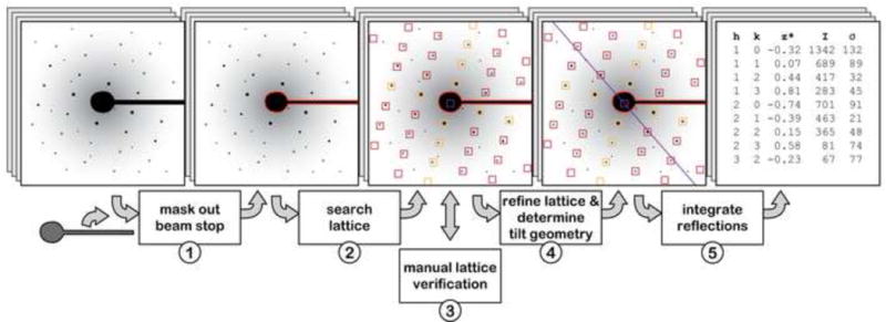
The intensity-extraction procedure of the IPLT diffraction-processing pipeline includes five steps. 1) Based on the user-defined shape of the beam stop, its position is automatically determined in each diffraction pattern. 2) The crystal lattice, including the origin, is automatically searched. 3) The determined lattice can be interactively verified by using the graphical data viewer, which also provides an efficient means to correct it if necessary. 4) The lattice is automatically refined using a lattice model that takes barrel and spiral distortions into account, after which the tilt geometry is determined based on the lattice vectors and the crystallographic unit cell. 5) To extract the reflection intensities, the area around each lattice peak is integrated and corrected for the background. The entire procedure can be automated to process a set of diffraction patterns at once, increasing the processing efficiency.
At the beginning of each project a polygonal shape is manually defined that describes the outline of the beam stop of the used electron microscope. The definition of the beam stop shape is conveniently done in the GUI, using one of the diffraction patterns as template. Once defined, the beam stop shape is automatically positioned on each diffraction pattern, which is more convenient than the manual method implemented in MRC/XDP.
Automated analysis of measured or calculated diffraction patterns requires the identification of the reflection peaks. A flexible and powerful peak search algorithm has been implemented in IPLT for this purpose. Its parameterization accounts for the expected peak spread and for better differentiation between signal and background. The latter results in a marked reduction in the number of identified false-positive peaks caused by noise. The algorithm can be applied in 1D, 2D and 3D peak searches, and a detailed description is provided in the Methods and Implementations section.
The lattice for each diffraction pattern is then automatically searched, based on the peak positions identified by the peak search (Figure 2). The lattice search includes determination of the lattice origin as well as lattice indexing that is consistent with the nominal tilt parameters known from data acquisition at the electron microscope. Compared to the manual method employed in XDP, these features greatly facilitate and speed up the indexing of diffraction patterns, especially of those recorded from tilted specimens. The correct indexing of the lattice can be verified using the graphical data viewer (see GUI section). The initial lattice found by the lattice search can be automatically refined by the use of a least squares-based algorithm. In addition to the refinement of the lattice vectors and the lattice origin, the algorithm also provides the option to determine and refine parameters for the correction of barrel and spiral distortions affecting the lattice.
Figure 2. Automatic lattice search and refinement.
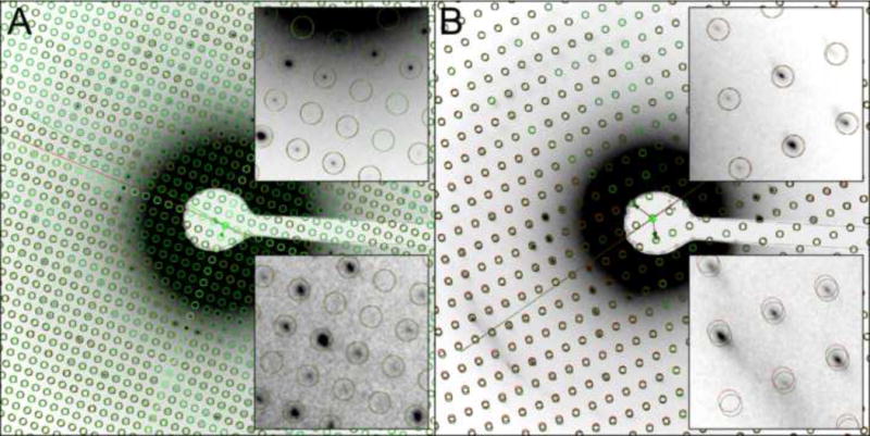
The lattice for each diffraction pattern is automatically searched and refined. The initial lattice identified by the lattice search step is shown in red, and the refined lattice in green. The orientation of the tilt axis is automatically determined based on the distortion of the lattice due to tilting of the sample plane. Panel (A) shows the initial and refined lattices overlaid on a diffraction pattern recorded from an untilted sample, and panel (B) shows the lattices overlaid on a diffraction pattern recorded from a sample tilted to 65°. The insets on the top right display a magnified view of a low-resolution area, and the insets on the bottom right display a magnified view of a high-resolution area. Lattice refinement is particularly important for the extraction of intensities of high-resolution reflections in diffraction patterns recorded from highly tilted samples (bottom right inset in panel (B)).
Once the lattice is refined, the reflection intensities are extracted by integration over the diffraction spots and correction for the background contribution. To determine the quality of the extracted intensities, the RFriedel factor is calculated for each diffraction pattern. The RFriedel value is also used as measure for the automated optimization of the radius used for integration.
1.2. Diffraction data merging
Once peak intensities have been extracted from a set of diffraction patterns, they have to be merged into a consistent 3D data set. Merging comprises the scaling of the peak intensities extracted from individual diffraction patterns, refinement of tilt geometry and fitting of lattice lines, followed by a discretization step. The data set can be iteratively refined to find optimal scaling and tilt parameters (Figure 3).
Figure 3. Merging of intensity data extracted from a set of diffraction patterns.
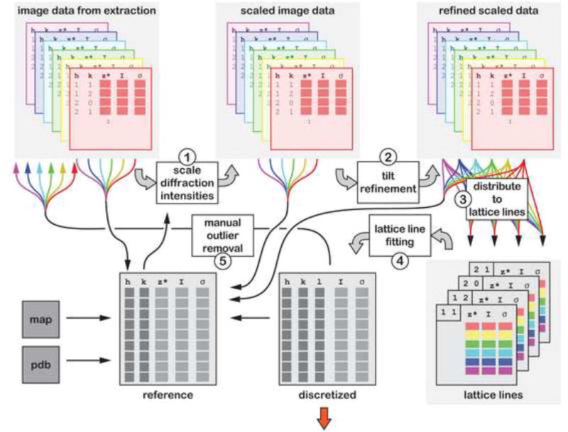
Merging of diffraction data with the IPLT pipeline comprises five steps that can be repeated iteratively to refine the merging parameters. 1) The scale and temperature factors are determined for the diffraction intensities extracted from a set of diffraction patterns to scale them to a common level. Reference data for scaling can either be taken from the original unscaled data, from a previous merging iteration (in the form of scaled, tilt geometry-refined or fitted data), or from an external reference. The reference data are either used directly in the form of individual reflections or as a resolution-binned intensity profile. 2) Based on the extracted diffraction intensities, the tilt geometry of each diffraction pattern is refined. 3) The refined tilt geometry is used to distribute the diffraction intensities along lattice lines. 4) Each lattice line can be fitted separately, allowing parallelization of the lattice-line fitting step. The fitted curves are discretized for further use as reference or for subsequent phasing (indicated by the red arrow). 5) The diffraction data and fitted lattice lines can be visually inspected using the lattice line viewer (Figure 5F) and outliers can be removed.
Scaling and temperature factors are determined to account for differences in intensity levels between different diffraction patterns. The flexible implementation of the IPLT scaling algorithm allows the use of different scaling references, such as unscaled reflection data, previously scaled reflection data, tilt geometry-refined reflection data, and even a density map or reflection data from an external reference. In contrast to the conventional common line scaling applied by the MRC programs, the IPLT pipeline provides the option of determining scale and temperature factors based on a resolution-binned intensity profile instead of the individual reflections, i.e., applying a Wilson-type scaling (Wilson, 1942). This option permits diffraction patterns of the full tilt range to be used as initial reference. The scaling module also allows separate temperature factors to be determined for the directions parallel and perpendicular to the tilt axis to account for anisotropy in the diffraction patterns. After merging the scaled data set, it is normalized to preserve the average intensity level within the full data set.
The initial values for tilt axis and angle of each diffraction pattern are refined against the scaled data set, and the resulting data set is normalized to avoid an overall stretching or compression of the data set along z*.
Lattice line fitting and discretization of the data set is performed by a multidimensional, non-linear least squares fit, which fits a sum of squared functions, each consisting of a sinc term multiplied by a complex factor, to the experimental intensity data set. Sparse areas or gaps in the data set are automatically taken care of during fitting. On a multiprocessor platform the lattice line fitting algorithm can fit several lattice lines in parallel.
1.3. Automation and optimization
Great care was taken to automate and optimize the IPLT processing pipeline to allow the processing of electron diffraction data in a time-efficient manner. Positioning of the beam-stop mask, determination of a lattice consistent with the nominal tilt geometry, lattice refinement, reflection integration, data merging, refinement of the merged data set, and lattice line fitting are all automated. IPLT only requires user input to verify the correctness of the determined lattice.
To further speed up data processing, the most time-consuming algorithms, i.e., lattice refinement, reflection integration and lattice line fitting, were re-implemented in a parallelized fashion.
To avoid the user from having to manually find the best set of parameters to extract the diffraction intensities, IPLT also includes an automatic procedure to optimize the radius that determines the size of the integrated reflection area. The integration algorithm allows diffraction intensities and error estimates of smaller sub-areas of the integration area to be calculated on the fly without reintegration of the peak areas. Therefore, each diffraction peak has to be integrated only once with the maximum radius. From the extracted intensity data the RFriedel factor can be calculated for any radius up to the maximal radius, and the optimal radius and the corresponding set of reflection intensities can be determined without reintegration of the reflection peaks. With the optimized lattice refinement and integration algorithms implemented in IPLT, lattice refinement, optimization of integration radius and data extraction took 38 s on a 2.8 GHz test machine, ~20 times faster than the implementation used in XDP (see Supplementary Information and Supplementary Information Figure 1).
Use of the automated and optimized algorithms together with an optimized data management strategy (see Section 2.2) allows efficient processing of big electron diffraction data sets.
1.4. Data quality
To assess the accuracy of the IPLT diffraction-processing pipeline, 276 diffraction patterns of AQP0 2D crystals grown with the lipid 1-stearoyl-2-oleoyl-sn-glycero-3-phosphatidylethanolamine were processed in parallel with both the IPLT and XDP diffraction processing pipelines. As XDP does not provide automatic lattice determination, the initial lattice parameters automatically determined in IPLT were also used for processing in XDP. Optimization of the box size used for peak integration was determined automatically in IPLT as described above, but had to be done manually in XDP. For each diffraction pattern, the RFriedel factor was calculated from the reflection intensities extracted by both processing pipelines. Comparison of the RFriedel values for reflections identified by both programs shows that the reflection data obtained with the IPLT pipeline are at least equally good as those obtained with the XDP pipeline (Figure 4). It should be noted, however, that 31% more reflections were picked up by IPLT than by XDP (Table 1, and see below).
Figure 4. Assessment of the quality of diffraction data extracted with the IPLT pipeline.
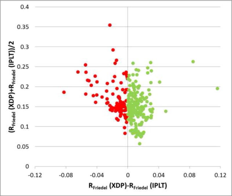
276 diffraction patterns of AQP0 2D crystals collected at tilt angles ranging from 0° to 70° were processed using the XDP/MRC software and the IPLT diffraction-processing pipeline. RFriedel factors were calculated for the two data sets, only including reflections that were identified by both XDP/MRC and the IPLT pipeline, hence ensuring an equal number of reflections for both RFriedel factor calculations. The equal number of reflections allows direct comparison of the RFriedel values for the extracted data and shows that XDP yielded lower RFriedel values for 93 diffraction patterns (red), whereas IPLT yielded lower RFriedel values for 183 diffraction patterns (green). Especially for good diffraction patterns with low RFriedel values, which are most likely to contain useful data to high resolution, the majority of patterns show a slightly lower RFriedel value when processed with IPLT.
Table 1. Assessment of the quality of diffraction data merged with the IPLT pipeline.
RMerge and RMeas statistics in resolution bins ranging from 100 Å to 2.5 Å for the data sets merged with the XDP/MRC software and the new IPLT processing pipeline. The table shows that the IPLT pipeline extracts ~31% more reflections than the XDP/MRC software, while still yielding better RMerge and RMeas values overall and in most resolution bins. Especially R-factors for data above a resolution of 3.33 Å improved by the use of the IPLT diffraction-processing pipeline.
| XDP | IPLT | ||||||
|---|---|---|---|---|---|---|---|
|
| |||||||
| Resolution bin (Å) | RMerge | RMeas | N | RMerge | RMeas | N | |
| 100.00 | 9.95 | 0.3159 | 0.3192 | 1411 | 0.3110 | 0.3129 | 6294 |
| 9.95 | 7.06 | 0.3233 | 0.3256 | 8006 | 0.3075 | 0.3095 | 10294 |
| 7.06 | 5.77 | 0.3477 | 0.3508 | 7950 | 0.3627 | 0.3654 | 10371 |
| 5.77 | 5.00 | 0.3263 | 0.3297 | 8429 | 0.3491 | 0.3526 | 10819 |
| 5.00 | 4.47 | 0.3180 | 0.3217 | 8645 | 0.3248 | 0.3283 | 10720 |
| 4.47 | 4.08 | 0.3041 | 0.3076 | 8636 | 0.3206 | 0.3239 | 10670 |
| 4.08 | 3.78 | 0.3273 | 0.3315 | 8743 | 0.3455 | 0.3495 | 11201 |
| 3.78 | 3.53 | 0.4046 | 0.4102 | 8580 | 0.4343 | 0.4397 | 10831 |
| 3.53 | 3.33 | 0.4609 | 0.4676 | 8242 | 0.4784 | 0.4852 | 10510 |
| 3.33 | 3.16 | 0.4445 | 0.4511 | 8486 | 0.4327 | 0.4387 | 10907 |
| 3.16 | 3.01 | 0.5913 | 0.6014 | 7796 | 0.5787 | 0.5877 | 10530 |
| 3.01 | 2.89 | 0.6188 | 0.6298 | 7444 | 0.5806 | 0.5908 | 9894 |
| 2.89 | 2.77 | 0.7004 | 0.7136 | 7308 | 0.6381 | 0.6510 | 9209 |
| 2.77 | 2.67 | 0.6903 | 0.7060 | 6174 | 0.5852 | 0.6016 | 7270 |
| 2.67 | 2.58 | 0.7423 | 0.7632 | 5036 | 0.6481 | 0.6675 | 7164 |
| 2.58 | 2.50 | 0.8309 | 0.8575 | 4607 | 0.7736 | 0.8027 | 5897 |
|
| |||||||
| Overall: | 0.3440 | 0.3478 | 115493 | 0.3347 | 0.3377 | 152581 | |
Merging and refinement of the data were also performed using both pipelines. The reflection data extracted with XDP were merged and refined using the XDP merging pipeline and the reflection data extracted using IPLT were merged and refined using the IPLT pipeline. As a result of this procedure, the merging outcomes also depend on the results of the extraction with the two programs. To allow for a fair comparison, the scale factor normalization implemented in IPLT was also added to the corresponding XDP script. This addition avoids scaling problems in XDP for a subset of diffraction patterns that lead to a continually decreasing scale factor for these patterns during the refinement iterations. Without the normalization, these patterns would have to be removed from the data set.
For the data merge in IPLT and XDP, RMerge and RMeas factors were calculated for the overall data and for a set of resolution bins (Table 1). The overall RMerge factors were 0.3347 for IPLT and 0.3440 for XDP. The less stringent filtering of the reflections in IPLT results in a 31% higher number of extracted reflection intensities (152,581 in IPLT versus 115,493 in XDP). The overall RMeas factors, which are corrected for sample multiplicity, were 0.3377 for the data set processed in IPLT and 0.3478 when it was processed in XDP (Table 1). The two R factor values clearly demonstrate that the automated IPLT processing pipeline is able to provide the same quality of data processing as the classical MRC/XDP software, while recovering more reflections. Of note, the additional diffraction intensities obtained by processing in IPLT result in improved RMeas factors in the resolution range from 3.33Å to 2.50Å.
2. Graphical user interface, data management, and software design
2.1. Graphical user interface
The “giplt_diffraction_manager” is the GUI for the IPLT diffraction-processing pipeline. If the giplt diffraction manager is opened within a folder that contains an IPLT diffraction project, it automatically loads the settings for that project. If it is opened in a directory that does not contain an IPLT diffraction project, it offers the choice of either opening an existing IPLT diffraction project in a different directory or of creating a new diffraction project. In the latter case, a wizard will collect all available information for the new project (unit cell parameters, symmetry, etc.) and will then guide the user through the remaining steps in the project creation process. Once a project is opened, the GUI is organized as three separate panels, labeled project, diffraction pattern, and merge.
The project tab displays all information relevant to the entire project (Figure 5A). It also allows changing of project-wide default parameters, addition of new diffraction patterns to the project, definition of the shape of the beam stop, and processing and merging of all diffraction patterns for an entire project.
Figure 5. Graphical user interface.
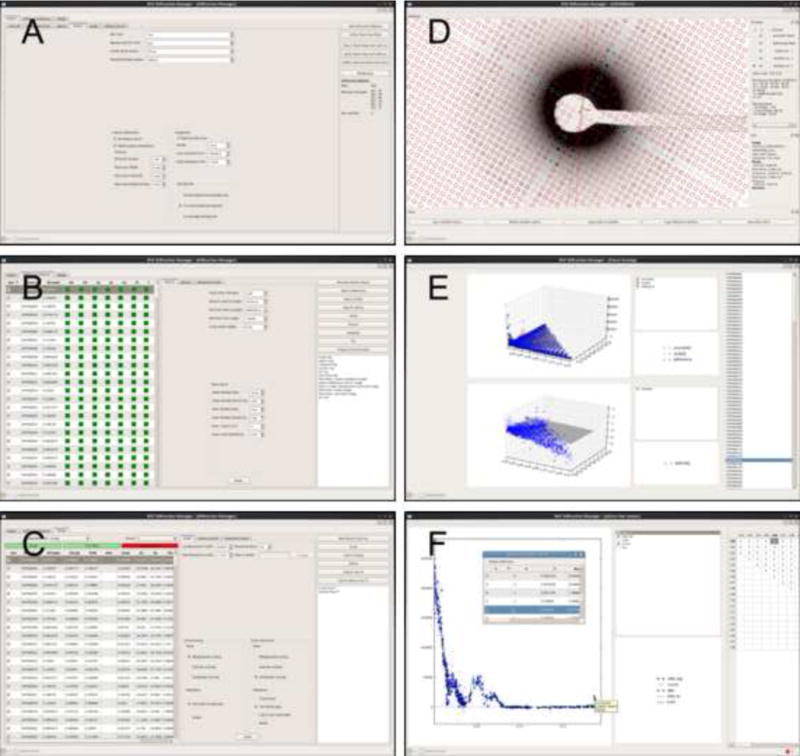
The GUI of the IPLT diffraction manager is organized as three panels. (A) The project panel is used to add new diffraction patterns to a project and to set project-wide parameters. (B) The diffraction pattern panel displays the processing status for each diffraction pattern and allows setting of pattern-specific parameters. (C) The merge panel organizes the merging and refinement of the diffraction data set. In addition to the three main panels, the IPLT diffraction manager features several widgets to display data during processing and refinement. (D) The data viewer displays diffraction patterns with overlaid processing data as for example lattices, beam stop mask, and extracted reflection data. (E) The scaling widget displays the fits used to determine the scale and temperature factors during merging. (F) The lattice line viewer displays the diffraction data and the fitted curve for each lattice line and allows easy identification and removal of outliers by using the integrated reflection list viewer (see inset). Larger views of these panels are provided as Supplementary Information Figures 2 to 7.
The diffraction pattern tab displays a table that lists all diffraction patterns included in the project (Figure 5B). This table provides an overview of the processing status of each diffraction pattern and also displays the RFriedel factors for diffraction patterns that are fully processed. The sorting feature of the table allows the user to easily identify diffraction patterns that are not fully processed or patterns of poor quality, which can be excluded from further processing at the user’s request. In addition, the diffraction pattern tab allows the user to override the default processing parameters for individual diffraction patterns, to manually process diffraction patterns, and to assess the processing results.
The merge tab facilitates the merging of a set of diffraction patterns into a 3D data set (Figure 5C). Since the IPLT diffraction-processing pipeline allows multiple merge instances, each merge instance is set up to reside within a dedicated directory. The merge instances themselves can be aggregates of multiple refinement cycles. The merging tab enables fine-grained control over the merging process. Diffraction patterns can be included in or excluded from individual merging instances or refinement cycles. In addition, it allows the user to easily judge the data and processing quality by providing RMerge values for the scaling and refinement steps as well as an interactive lattice line viewer to inspect the lattice lines fitted to the data.
The GUI has an extendable architecture that allows the user to add custom tabs that can provide functionality beyond the ones provided by default. For example, this feature was used to add an XDP custom exporter that can write out diffraction patterns and their lattices in an XDP-compatible format.
Interactive data viewer
The interactive data viewer is a central component of the IPLT diffraction processing GUI. It provides a wealth of potent features and sophisticated functionalities: (i) Memory-efficient graphical implementation allows fast translation and zooming, independent of the actual size of the diffraction pattern. (ii) Above a certain magnification scale, numerical values are displayed on each pixel. (iii) Mapping of pixel values to grey scale can be adjusted either manually or based on an interactively selected sub-region within a diffraction pattern. (iv) Data determined during the processing, such as the lattice or the reflection intensities, can be displayed by using overlays within the data viewer (Figure 5D).
Auxiliary sub-windows complement the main image view with additional features. For diffraction patterns, an info panel provides information about the mouse position and the current selection box. If at least one overlay is present, the overlay manager subwindow allows overlays to be activated, toggled on or off, and their parameters to be modified through overlay-specific submenus.
Overlays
Overlays serve as flexible extensions to the image viewer to provide GUI elements for a multitude of tasks. Their implementation in IPLT was described in Philippsen et al. (2007). Overlays allow graphical elements to be drawn on top of an image displayed in the viewer, thus decoupling algorithm-specific graphical displays from the generic image display. The overlays are constructed and assembled in a dynamic and interactive way through the Python shell. Their parameters can be set and retrieved through their Python representation or through a graphical menu that is provided by the overlay manager subwindow in the image viewer (see above). Several overlays can be added to a single image viewer as illustrated in Figure 5D. The diffraction-processing pipeline makes use of several overlay options.
Lattice overlay: The lattice overlay provides the options to display and interactively fit a 2D lattice. The lattice is defined by an origin, two lattice vectors, and values for barrel and spiral distortions. In addition, if the unit cell parameters are known, the tilt geometry is also displayed and adjusted automatically if the lattice is changed. The lattice can be modified interactively by dragging individual lattice points around with the mouse. Up to two lattice points can be anchored to prevent them from moving during lattice adjustment. Although the adjustment of individual lattice points allows efficient tweaking of the lattice parameters, manual placement of a point on a peak in the diffraction pattern is inaccurate. The lattice overlay therefore provides automatic peak fitting of the lattice point that is being adjusted: with a single key press the peak center of the current lattice point is fitted with sub-pixel precision and the center of the lattice point is set to the determined center of the peak. The 2D Gaussian fit initially developed for lattice refinement is re-used for fitting the peak center in the lattice overlay, illustrating the advantage of the modular structure of IPLT. As algorithms are independent from image input/output (IO) and are not hard-coded into one specific executable, they can easily be used in contexts different from the originally intended use.
Point list overlay: The point list overlay allows a list of points to be displayed on top of a diffraction pattern. It is typically used to visualize the results of a peak search.
Mask overlay: The mask overlay is used to display polygonal masks, and it can be used to create a new polygon to define a mask or to modify the nodes of an existing mask. In the diffraction-processing pipeline, the mask overlay is used to define and display the mask for the beam stop.
Plot viewer
IPLT is equipped with an interactive plot viewer to display 2D Cartesian data sets. The plot viewer widget allows multiple data sets to be displayed within one plot. It adds legends for easy identification of the data sets as well as a data set list with which individual data sets can be shown or hidden. The mouse can be used to move the plot and for zooming. The zooming functionality can either act on the X axis, the Y axis, or both axes together. Clicking on a data point displays additional information. There is also limited support for polar 2D and Cartesian 3D data sets, but moving and zooming have not yet been implemented for such data sets. The IPLT diffraction-processing pipeline uses the plot viewer to display data within the scaling widget and the lattice line viewer.
Scaling widget: The scaling widget provides a visual display of the fit used to determine the scale and temperature factors for each diffraction pattern (Figure 5E). For each diffraction pattern, the scaling widget can show in one plot the diffraction intensities of the input data I, the reference data Iref, and the output data after scaling Iscaled, plotted against 1/resolution2. In a second plot, ln(I/Iref) is plotted against 1/resolution2. For isotropic scaling, both plots are 2D Cartesian plots, and for anisotropic scaling both plots are 3D Cartesian plots.
Lattice line viewer: The interactive lattice viewer allows the quality of the lattice line fitting to be assessed. Individual lattice lines can be selected using the grid displayed on the right (Figure 5F). To the left, a scatter plot displays all diffraction intensities of the selected lattice line, together with the fitted curve. Clicking on a data point pops up a tooltip window that displays additional information, such as the number of the source pattern from which the diffraction intensity was extracted. Double-clicking on a data point opens a reflection list editor for the corresponding diffraction pattern that allows the selected intensity to be deleted. This feature is useful to remove outliers caused, for example, by spurious signals due to cosmic rays or sample contamination by crystalline ice, sugar or salt. The interactive lattice line viewer is crucial for efficient data processing because it provides a direct link between the lattice-fitted data and the unscaled raw data coming from the diffraction patterns. This link is lost with the conventional way of plotting lattice lines to a file.
2.2. Data management
As generally true in image processing, the use of proper data management strategies is also critical for efficient processing of electron diffraction data. The strategy used in IPLT diffraction processing includes the choice of a clear directory structure for organizing the generated data as well as log files, a hierarchical parameter storage concept in the portable xml file format, and a caching infrastructure to avoid unnecessary disk IO.
The directory structure adopted for IPLT diffraction processing consists of a root directory containing project-wide configuration data, and subdirectories for each recorded diffraction pattern and for each merging run.
Diffraction pattern meta-data (tilt geometry, lattice, etc.) and diffraction processing parameters are represented in a tree-like info hierarchy (see Philippsen et al. (2007) for implementation). IPLT diffraction processing employs a two-level hierarchy of configuration files. The top-level configuration file (project.xml) contains project-wide meta-data (e.g., unit cell definition of the 2D crystal) and the default values for all processing parameters. In addition, each diffraction pattern and merge subdirectory contains a second configuration file (info.xml) that only contains diffraction pattern-specific meta-data (e.g., lattice) as well as processing parameters that differ from the default values. During processing, parameters that are not included in the diffraction pattern-specific configuration file are read from the project-wide configuration file. This design presents the user with a transparent and straightforward parameter organization, and it avoids duplication of parameters and the need to synchronize between different configuration files.
Overall processing speed can be greatly increased by complementing the data-processing algorithms with a caching infrastructure. IPLT diffraction processing deviates here from the classical approach of chaining a series of executables together using a shell script. Instead, the processing procedures are implemented as Python modules that make use of low-level C++ algorithms. After application of an algorithm, rather than writing the processed data to disk and then re-reading the data from disk for the next algorithm, IPLT keeps these data in memory by using a central data manager that organizes the handles for diffraction pattern and reflection data (Figure 6). In addition to the performance gain, caching directly within IPLT also avoids normalization and data conversion steps normally performed to write and read data to and from a storage medium, which can introduce rounding artifacts.
Figure 6. Data management.
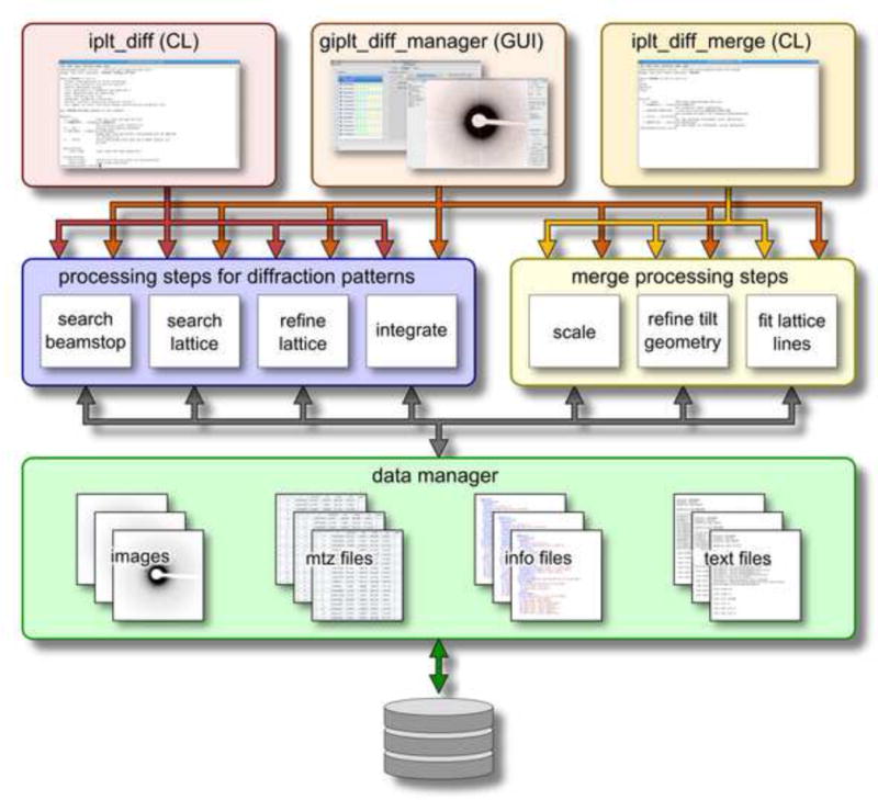
The IPLT diffraction-processing pipeline provides a graphical user interface, giplt_diff_manager, and two command line interfaces on the top level, iplt_diff for extracting reflection intensities from diffraction patterns and iplt_diff_merge for the merging of electron diffraction data. Both interfaces use the same set of intermediate-level Python processing modules to ensure consistent processing between GUI and command line, and to avoid code duplication. On the low level, the processing modules access a central data manager to retrieve and store image, reflection, text, and xml data, which allows extensive caching and re-use of data for multiple processing steps.
In addition to diffraction pattern and reflection data, meta-data, parameters and log output are also cached. Parameter and meta-data caching improves performance as these are often accessed from different places within the diffraction-processing pipeline and the GUI.
2.3. Software design
The current version of IPLT is built on the OpenStructure framework for Computational Structural Biology (OST; www.openstructure.org) (Biasini et al., 2010), calling upon OST’s framework for Computational Structural Biology and its core image storage and processing capabilities, its display widgets, and its extensive IO functionality. The image IO module supports a wide range of image file formats, including the mrc, ccp4, spider, dm3, situs and ipl formats, and it is therefore able to handle almost all image data generated in the EM community.
The diffraction-processing pipeline consists of a set of algorithms implemented in C++ that are linked by a set of high-level processing modules in Python and a GUI. Implementation of the GUI is based on the Qt toolkit (qt-project.org), which uses the native graphics application programming interface on Linux, OSX and Windows (note that it is therefore not necessary to run X-Windows on an OSX or Windows machine to use IPLT).
The diffraction-processing pipeline is distributed as part of the IPLT distribution, which is available as source code and binary packages for Linux, OSX and Windows at www.iplt.org.
Conclusions
The diffraction-processing pipeline in IPLT provides an automated way to process large electron diffraction data sets. Processing of diffraction patterns with IPLT incorporates more reflections and produces a merged 3D data set with a quality that is similar or slightly better than when the same patterns are processed with the MRC programs (Table 1). Because of the automation of all essential processing steps and the streamlined user interface that allows the user to quickly assess the data quality and, if necessary, to easily correct mistakes, data processing is easier and much faster with the IPLT pipeline.
IPLT supports a large number of image and reflection file formats, and it can thus interface with a wide range of image processing software. Furthermore, the modular design of IPLT and its diffraction-processing pipeline that uses a combination of C++ and Python make it easy to implement new algorithms and processing strategies. The two popular programming languages C++ and Python were chosen for the implementation of the IPLT diffraction-processing pipeline specifically to allow the wider community to contribute to the code. As IPLT is based on OpenStructure, the computational structural biology framework, there is great potential for further extension of IPLT by using the tools of OpenStructure for manipulating and displaying molecular structures.
The pipeline for efficient processing of electron diffraction data implemented in IPLT will reduce the overall time needed to determine the structure of a protein by electron crystallography. In addition, because of the automation, data can be processed at the same time when new data are being collected, thus providing fast feedback on the quality of the data that are being recorded. These factors will allow more extensive electron crystallographic studies to be performed within a reasonable amount of time. Examples would be electron diffraction studies of membrane proteins in different functional states (e.g., Subramaniam & Henderson, 1999), of membrane proteins carrying mutations (e.g., Subramaniam et al., 1999), or of lipid-protein interactions (Gonen et al., 2005; Hite et al., 2010a; Schenk et al., 2010a).
Methods & Implementation
1. Protein purification, crystallization and data collection
The core tissue of sheep lenses (Wolverine Packing Company, Detroit, MI) was dissected away from the soft cortical tissue, and membranes were prepared as previously described (Gonen et al., 2004). AQP0 was purified from the membranes as previously described (Hite et al., 2010a). Purified AQP0 was reconstituted into 2D crystals using 1-stearoyl-2-oleoyl-sn-glycero-3-phosphatidylethanolamine (Avanti Polar Lipids) at a lipid-to-protein ratio of 0.4 (mg/mg) by dialysis against 10 mM MES, pH 6, 150 mM NaCl, and 50 mM MgCl2 at 37°C for 5 days.
Specimens for collection of electron diffraction patterns were prepared using the carbon sandwich technique (Gyobu et al., 2004), and diffraction patterns were recorded on an FEI Tecnai G2 Polara as previously described (Hite et al., 2010a).
2. Diffraction data extraction
2.1. Beam stop determination
The position of the beam stop in a diffraction pattern is determined by a cross correlation-based search of the beam stop shape, as manually defined by a polygonal beam stop mask, within a filtered version of the diffraction pattern. To create the filtered diffraction pattern the user has a choice of either using i) a clipping algorithm, for which the minimum and maximum values are determined by a histogram analysis, ii) a Gaussian filter (see Supplementary Information), or iii) a local sigma thresholding algorithm.
2.2. Lattice determination
The position of a lattice point is based on its (h,k) indices and is given by , where is the origin and are the two reciprocal lattice vectors. The lattice search can be divided into four conceptually separate steps, which are: i) a peak search to identify the diffraction reflections, ii) determination of an initial set of lattice vectors , iii) determination of the lattice origin , and iv) adjusting the lattice vectors to be consistent with the tilt geometry.
i) Peak search
The task of a peak search is to identify a set of candidate lattice peaks in a diffraction pattern. It also serves as a data-reduction step, decreasing the data from a full-sized diffraction pattern to a set of peak coordinates. A detailed description of the peak search algorithm is provided in the Supplementary Information.
ii) Lattice vector determination
The lattice vectors of a diffraction lattice are determined by using a difference-vector algorithm based on the method described in Kabsch (1993). In a first step, a peak search is performed, and the parameters used in the peak search algorithms (sensitivity and peak size) are automatically refined according to the number of peaks found. Optimization is needed to avoid too many peaks (likely to introduce more noise peaks) or too few peaks. From this peak list, the distance vector between each pair of peaks is calculated. All these distance vectors contribute to a new image, the vector image. The vector image is generated starting from an image with all the pixel values set to zero. The pixel value is increased at each position of the image (index) defined by the components of the distance vectors. To increase the precision of the determined lattice, difference vectors, which in general have non-integer x and y values, contribute to all four pixels surrounding the exact vector positions by linear interpolation. On this vector image a second peak search is performed, and a second vector image is generated from these peaks. In this second vector image, the two closest points to the center that are not collinear are taken as a first guess for the lattice vectors.
iii) Origin determination
The correct lattice origin is determined in three steps: i) the geometric center of all peaks determined during the peak search is calculated. ii) Centering the lattice at the geometric center, the average offset from the nearest lattice point of all peaks is determined, and the lattice is shifted to minimize the average distance. iii) Starting from this refined origin the sum of the weighted difference of Friedel-related peaks is calculated for a set of lattice origins with −20 ≤ h, k ≤ 20. The peaks are weighted based on their proximity to the nearest lattice point. The origin yielding the lowest difference sum is used as final lattice origin.
iv) Lattice vector adjustment
There are several equally valid possibilities for to index a given lattice, which cannot be distinguished from the peak information itself. Therefore, additional knowledge about the data acquisition conditions has to be used to identify the correct indexing. IPLT determines the most likely indexing based on the nominal tilt angle βn and the nominal position of the tilt axis αn, which are known to a certain degree of error from the data acquisition conditions, and the tilt angle β and position of the tilt axis α as determined from the lattice using the method described in Shaw and Hills (1981). The optimal lattice is defined as the lattice minimizing f as given in (1):
| (1) |
The weighting factor w allows the weight of the axis angle with respect to the tilt angle to be adjusted depending on how well it is defined by the microscope. For microscopes in which the tilt axis position is random, the weight can be set to 0. The lattice vector adjustment uses the set of vectors determined by the lattice search as starting vectors for the initial round (n = 0) of an iterative refinement of the lattice vectors. It then determines the four candidate sets of vectors , and and calculates f for each of them. The candidate set with the lowest f is taken as starting set for the next iteration. The iteration stops once all candidate sets give a higher value for f than the starting set for that iteration.
2.3. Lattice refinement
The more complex lattice model used for lattice refinement includes barrel and spiral distortions, which are defined by two constants, Kb and Ks, and are given by (2)
| (2) |
For lattice refinement, the lattice determined during lattice search is superimposed on the original image. At each of the predicted lattice points, a 2D Gaussian function (see Supplementary Information) is fitted to determine the exact position of the potential peak. This list of positions is fed into the lattice refinement algorithm, which determines the best set of lattice parameters for Eq. (2). If both barrel and spiral distortions are set to zero, a linear least-squares routine is used, but otherwise a more involved, non-linear least-squares routine is employed. Both variants are implemented using a Levenberg-Marquardt algorithm from the Gnu Scientific Library (Galassi, 2009). The lattice refinement algorithm can also be called as a stand-alone routine outside the context of the lattice search algorithm.
2.4. Data extraction
For extraction of intensity values, the background-corrected intensity for each peak is calculated. The average background Bg(h,k,r) is determined by integrating the pixel values V((x,y)) with pixel positions (x,y) over a ring R with width dbg according to equation (3),
| (3) |
where rbg is the outer radius equal to half the shortest distance between two reflection peaks (see Supplementary Information Figure 8), and l is the peak position of index (h,k), according to equation (2).
The peak intensity I(h,k,r) is determined in a similar way by integration across a circle C around the peak center according to equation (4):
| (4) |
The user can select whether the error estimate for each integrated diffraction intensity is determined from the intensity fluctuation within the background ring around the reflection peak or from the similarity of Friedel-related spots.
During data extraction the radius r is automatically optimized within a user-given range. The peak intensities are calculated for each box radius within the search range, and the data set yielding the highest overall is used for further processing, with being the average amplitude of all extracted peaks. The use of the area integrator algorithm (see Supplementary Information for implementation details) allows each peak area to be integrated only once for the biggest radius in the search range. All peak intensities for smaller radii can then be calculated on the fly over the smaller peak areas without re-integration.
3. Diffraction data merging
3.1. Scaling
The reference data for the scaling algorithm can either come from a resolution-binned intensity profile or from a set of reference reflections. Both types of references can either be calculated from an initial merged and unscaled data set, a refined data set from a previous refinement cycle, or an external reference in the form of a density map or a set of structure factors.
The scaling and temperature factors are refined using a linear least-squares fit according to Ceska and Henderson (1990) with:
| (5) |
for isotropic scaling and:
| (6) |
for anisotropic scaling, where Iref are the reference intensities, Iobs are the observed intensities, S is the scale factor, d is the distance of a reflection peak from the center of the diffraction pattern, d⊥,d|| are the distance components perpendicular and parallel to the tilt axis, B is the isotropic temperature factor, and B⊥,B|| are the anisotropic temperature factors perpendicular and parallel to the tilt axis. After determination of the scaling and temperature factors, the scaled amplitudes Iscaled can be calculated as follows:
| (7) |
and:
| (8) |
After scaling refinement the data set is normalized according to:
| (9) |
| (10) |
| (11) |
where n is the number of diffraction patterns, Snorm is the scaling normalization factor, Bnorm is the temperature normalization factor, and Inorm is the intensity after normalization.
3.2. Tilt geometry refinement
The initial tilt geometry for each diffraction pattern is calculated from its lattice distortion using the algorithm outlined in Shaw and Hills (1981). The parameters for tilt axis and angle are then refined using a Nelder-Mead simplex algorithm (Nelder and Mead, 1965) with the RMerge of the diffraction data set versus the scaled and merged data set as target function.
Normalization
Normalization prevents stretching or compression along the z* axis during iterative refinement by multiplying all z* values of the tilt geometry refined data set for refinement round r by fnorm(r), which can be calculated based on the tilt angle ßi for each diffraction pattern. n is the number of diffraction patterns.
| (12) |
3.3. Lattice line fitting
For a bandwidth-limited, discretized function in real space, the resulting Fourier space is sufficiently described by a finite number of complex coefficients . If these coefficients were known for a particular lattice line, the central-section intersection value Fhk at a particular z* for a crystal with thickness c could be calculated by equation (13).
| (13) |
For a function Fhk(z∗) discretized at a regular interval, zn can be substituted by n/ND with N being the number of samples in z direction and D being the distance between two sample points. Equation (13) can then be rewritten as:
| (14) |
What is measured in reality is the intensity at each z*, i.e., I = |F|2
| (15) |
Defining , equation (15) can be written as:
| (16) |
The parameters of equation (16) are adjusted to best fit a set of experimental data points (Ii, zi*) by minimizing the sum S of squared residuals
| (17) |
using an Levenberg-Marquardt non-linear least-squares fitting algorithm (Levenberg, 1944) provided by the Gnu Scientific Library (Galassi, 2009). The discretized intensities can subsequently be obtained from the complex coefficients: . The initial guess for a set of coefficients is generated by calculating the average amplitude for each n by averaging the intensities of all experimental data points within the window and taking the square root. The phase φ is either randomized or set to zero. The algorithm automatically takes care of missing high-resolution data or sampling gaps in the data by excluding windows from fitting, in which the number of experimental data points falls below a user-defined threshold. With lattice lines being independent of each other, the fitting of lattice lines was parallelized using QtConcurrent. If present, the lattice line fit makes use of the hermitian symmetry.
Because the non-linear least squares are in general not globally concave, optimization is not guaranteed to converge, and the sum of squared residuals S may contain multiple local minima. To assign a measure of accuracy to the sample estimates, a bootstrapping method is used for several iterations of the lattice line fitting procedure, in which data are resampled with replacement, yielding a resampled data set of the same size as the initial data set.
4. R-factor calculation
The IPLT diffraction-processing pipeline uses R-factors to measure the agreement between the experimental data and a reference. The basic formula is always the same, with a sum over an intensity difference divided by a sum over intensities.
| (18) |
In contrast to R-factors used in x-ray crystallography (Blundell and Johnson, 1976), in electron crystallography, the intensities in the nominator are not used as their absolute values, but rather carry their sign with them, which is a consequence of background correction that allows intensities to go into the negative regime for the purpose of proper error distribution around the zero intensity line. In essence, the R-factors differ in the definition and calculation of their reference intensity Iref, which are explained in the following paragraphs.
4.1. RFriedel
RFriedel is the simplest and most readily available R-factor for individual diffraction patterns. As I (h,k,z*) = I(–h,–k,–z*), the majority of reflections have a Friedel mate in the pattern (except when obstructed by the beam stop). The reference intensity Iref in the above formulas then simply becomes the average between the Friedel mates .
| (19) |
RFriedel is an excellent measure for the quality of an individual diffraction pattern, as it is independent of the tilt geometry or any other data. As RFriedel is influenced by the parameters used for intensity integration, it allows fine-tuning of these parameters.
4.2 RMerge
In x-ray crystallography, a single reflection defined by an (h,k,l) triplet may be (and usually is) present multiple times in a data set. In the case of electron crystallography, the uneven distribution of intensity measurements along the lattice lines along z* requires a different approach to estimating the quality of a merge. For each reflection, a local window average from closely neighboring reflections on the same lattice line is calculated, and this average is then used as the reference value in the R-factor calculation:
| (20) |
The width of the local window (in Å-1) is set manually by the user. It should correspond roughly to the inverse thickness of the crystal sample.
RMerge can be calculated as soon as data from different diffraction patterns are combined. It can monitor the quality of scaling, it can be used as a target for tilt geometry refinement, it can serve as a filter to eliminate patterns that clearly do not fit the overall data set, and it allows determination of the high-resolution cutoff for the final reflection list.
4.3. RMeas
Because the RMerge value calculation has an implicit dependence on the redundancy of the data, IPLT also allows calculation of RMeas, a corrected R-factor that can be used as a robust indicator for data consistency even for highly redundant data sets (Diederichs and Karplus, 1997), which is often the case in electron diffraction studies. RMeas is calculated as follows:
| (21) |
where nwin is the number of reflections within the averaging window.
5. Framework
The diffraction-processing pipeline is built based on the tools provided by the IPLT image processing toolkit. IPLT consists of a hybrid C++/Python architecture (Philippsen et al., 2007), which allowed implementing the diffraction-processing algorithms in C++ for optimal performance while still retaining the ability to easily combine the algorithms into a processing pipeline by using Python scripts. Each step of the diffraction processing is implemented as an individual Python module, which can be accessed either from the command line or the GUI. The input and output of image data, reflection list data, meta data, and log files are decoupled from the processing modules and are handled by a central data manager.
5.1. OpenStructure integration
The modules containing the basic geometry classes, the image handle, the general image algorithms, the image IO, the Python shell and the graphical data viewer that were part of the former standalone IPLT package (Philippsen et al., 2007) were integrated into the OpenStructure framework (Biasini et al., 2010). The electron crystallography-specific functionality was retained within the IPLT package.
5.2. Reflection data
Reflection data are organized using a reflection list handle, the conceptual design of which is similar to the image handle already presented in Philippsen et al. (2007). The reflection list is implemented as a multi-map of reflections using a reflection index with integer h and k and fractional z* values. The reflection data can have an arbitrary number of (floating point) properties. These properties are defined at the level of the reflection list. As such, a reflection list can be conceptualized as a table, in which the rows contain the individual reflections, and the columns the properties. Each column is assigned a data type following the conventions introduced by the ccp4 mtz file format (Winn et al., 2011). Similar to the image handle interface, the reflection list interface also supports the concept of algorithms that can be applied to reflection data. The IO for reflection list data supports the mtz and text file formats commonly used by the MRC software package (Crowther et al., 1996).
5.3. Data manager
The data manager for IPLT diffraction processing is implemented in Python using a singleton design pattern. It implements four separate write-back caches for image data, reflection list data, info handles, and log files. For each of the cache instances the maximal amount of cached data can be given separately for fine-grained control. This allows, for example, to cache a greater number of xml files containing parameters during merging for fast access to the crucial parameters, while still allowing for reflection list data to be flushed to disk relatively often. For data known to be accessed frequently (e.g., the main configuration file for a project) the caches provide a locking mechanism to avoid eviction of the data from the cache. The caches maintain a time stamp for each cache entry to ensure that data are written to the disk in the same order as they were written to the cache. The data manager provides an interface to flush the caches to disk at any time, and it ensures that all cached data are written to disk upon termination of the program.
6. Graphical user interface
The majority of the GUI was implemented using the PyQt4 (www.riverbankcomputing.com) Python wrapper to the Qt4 toolkit (qt-project.org) with some performance-sensitive widgets such as, for example, the data viewer and overlays being implemented in C++/Qt4. The IPLT diffraction manager makes use of the graphical python shell, dockable windows, and the logging facility implemented for the GUI of OpenStructure. A more detailed description of the GUI implementation can be found in Supplementary Material.
Supplementary Material
Acknowledgments
We thank Valerio Mariani, Marco Biasini and Gian-Andrea Signorell for their contributions to the IPLT software, and Richard K. Hite, Po-Lin Chiu and Manish Kumar for testing the IPLT diffraction-processing pipeline and providing critical feedback. We would also like to thank all the people that contributed to the MRC programs and its various additions, as the algorithms implemented in these programs were inspiration for many of the algorithms implemented in IPLT. The work on IPLT described in this manuscript was supported by the National Center of Competence in Research (NCCR) of Structural Biology, the European Union (EU projects LSHG-CT-2004-502828 and LSHG-CT-2005-018811), and the Maurice E. Müller Foundation of Switzerland to A.E. The development of the IPLT diffraction-processing pipeline was supported by Swiss National Science Foundation fellowships for Advanced researchers (126253 and 136484) to A.D.S. Electron crystallographic work on AQPs in the Walz laboratory was supported by NIH grants R01 EY015107 (to T.W.) and U54 GM094598 (to David Stokes). T.W. is an investigator with the Howard Hughes Medical Institute.
Footnotes
Publisher's Disclaimer: This is a PDF file of an unedited manuscript that has been accepted for publication. As a service to our customers we are providing this early version of the manuscript. The manuscript will undergo copyediting, typesetting, and review of the resulting proof before it is published in its final citable form. Please note that during the production process errors may be discovered which could affect the content, and all legal disclaimers that apply to the journal pertain.
References
- Abeyrathne PD, Chami M, Pantelic RS, Goldie KN, Stahlberg H. Preparation of 2D crystals of membrane proteins for high-resolution electron crystallography data collection. Methods Enzymol. 2010;481:25–43. doi: 10.1016/S0076-6879(10)81001-8. [DOI] [PubMed] [Google Scholar]
- Agemark M, Kowal J, Kukulski W, Nordén K, Gustavsson N, et al. Reconstitution of water channel function and 2D-crystallization of human aquaporin 8. Biochimica et Biophysica Acta (BBA)-Biomembranes. 2012 doi: 10.1016/j.bbamem.2011.12.006. [DOI] [PubMed] [Google Scholar]
- Biasini M, Mariani V, Haas J, Scheuber S, Schenk AD, et al. OpenStructure: a flexible software framework for computational structural biology. Bioinformatics. 2010;26:2626–2628. doi: 10.1093/bioinformatics/btq481. [DOI] [PMC free article] [PubMed] [Google Scholar]
- Blundell TL, Johnson L. Protein Crystallography. Academic Press; 1976. [Google Scholar]
- Brilot AF, Chen JZ, Cheng A, Pan J, Harrison SC, et al. Beam-induced motion of vitrified specimen on holey carbon film. J Struct Biol. 2012;177:630–637. doi: 10.1016/j.jsb.2012.02.003. [DOI] [PMC free article] [PubMed] [Google Scholar]
- Campbell MG, Cheng A, Brilot AF, Moeller A, Lyumkis D, et al. Movies of ice-embedded particles enhance resolution in electron cryo-microscopy. Structure. 2012;20:1823–1828. doi: 10.1016/j.str.2012.08.026. [DOI] [PMC free article] [PubMed] [Google Scholar]
- Casagrande F, Harder D, Schenk A, Meury M, Ucurum Z, et al. Projection structure of DtpD (YbgH), a prokaryotic member of the peptide transporter family. J Mol Biol. 2009;394:708–17. doi: 10.1016/j.jmb.2009.09.048. [DOI] [PubMed] [Google Scholar]
- Casagrande F, Ratera M, Schenk AD, Chami M, Valencia E, et al. Projection structure of a member of the amino acid/polyamine/organocation transporter superfamily. J Biol Chem. 2008;283:33240–33248. doi: 10.1074/jbc.M806917200. [DOI] [PMC free article] [PubMed] [Google Scholar]
- Ceska TA, Henderson R. Analysis of high-resolution electron diffraction patterns from purple membrane labelled with heavy-atoms. J Mol Biol. 1990;213:539–60. doi: 10.1016/S0022-2836(05)80214-1. [DOI] [PubMed] [Google Scholar]
- Chen JZ, Settembre EC, Aoki ST, Zhang X, Bellamy AR, et al. Molecular interactions in rotavirus assembly and uncoating seen by high-resolution cryo-EM. Proc Natl Acad Sci U.S.A. 2009;106:10644–10648. doi: 10.1073/pnas.0904024106. [DOI] [PMC free article] [PubMed] [Google Scholar]
- Crowther RA, Henderson R, Smith JM. MRC Image Processing Programs. J Struct Biol. 1996;116:9–16. doi: 10.1006/jsbi.1996.0003. [DOI] [PubMed] [Google Scholar]
- Diederichs K, Karplus PA. Improved R-factors for diffraction data analysis in macromolecular crystallography. Nat Struct Biol. 1997;4:269–275. doi: 10.1038/nsb0497-269. [DOI] [PubMed] [Google Scholar]
- Galassi M. GNU scientific library : reference manual Network Theory. 2009. Bristol. [Google Scholar]
- Gipson B, Zeng X, Zhang ZY, Stahlberg H. 2dx–user-friendly image processing for 2D crystals. J Struct Biol. 2007;157:64–72. doi: 10.1016/j.jsb.2006.07.020. [DOI] [PubMed] [Google Scholar]
- Glaeser RM, Downing KH. Specimen charging on thin films with one conducting layer: discussion of physical principles. Microsc Microanal. 2004;10:790–796. doi: 10.1017/s1431927604040668. [DOI] [PubMed] [Google Scholar]
- Glaeser RM, Hall RJ. Reaching the information limit in cryo-EM of biological macromolecules: experimental aspects. Biophys J. 2011;100:2331–2337. doi: 10.1016/j.bpj.2011.04.018. [DOI] [PMC free article] [PubMed] [Google Scholar]
- Glaeser RM, Baldwin J, Ceska TA, Henderson R. Electron diffraction analysis of the M412 intermediate of bacteriorhodopsin. Biophys J. 1986;50:913–920. doi: 10.1016/S0006-3495(86)83532-9. [DOI] [PMC free article] [PubMed] [Google Scholar]
- Gonen T, Sliz P, Kistler J, Cheng Y, Walz T. Aquaporin-0 membrane junctions reveal the structure of a closed water pore. Nature. 2004;429:193–197. doi: 10.1038/nature02503. [DOI] [PubMed] [Google Scholar]
- Gonen T, Cheng Y, Sliz P, Hiroaki Y, Fujiyoshi Y, et al. Lipid-protein interactions in double-layered two-dimensional AQP0 crystals. Nature. 2005;438:633–638. doi: 10.1038/nature04321. [DOI] [PMC free article] [PubMed] [Google Scholar]
- Gyobu N, Tani K, Hiroaki Y, Kamegawa A, Mitsuoka K, et al. Improved specimen preparation for cryo-electron microscopy using a symmetric carbon sandwich technique. J Struct Biol. 2004;146:325–333. doi: 10.1016/j.jsb.2004.01.012. [DOI] [PubMed] [Google Scholar]
- Henderson R, Unwin PN. Three-dimensional model of purple membrane obtained by electron microscopy. Nature. 1975;257:28–32. doi: 10.1038/257028a0. [DOI] [PubMed] [Google Scholar]
- Henderson R, Baldwin JM, Ceska TA, Zemlin F, Beckmann E, et al. Model for the structure of bacteriorhodopsin based on high-resolution electron cryo-microscopy. J Mol Biol. 1990;213:899–929. doi: 10.1016/S0022-2836(05)80271-2. [DOI] [PubMed] [Google Scholar]
- Hiroaki Y, Tani K, Kamegawa A, Gyobu N, Nishikawa K, et al. Implications of the aquaporin-4 structure on array formation and cell adhesion. Journal of Molecular Biology. 2006;355:628–639. doi: 10.1016/j.jmb.2005.10.081. [DOI] [PubMed] [Google Scholar]
- Hite RK, Li Z, Walz T. Principles of membrane protein interactions with annular lipids deduced from aquaporin-0 2D crystals. EMBO J. 2010a;29:1652–1658. doi: 10.1038/emboj.2010.68. [DOI] [PMC free article] [PubMed] [Google Scholar]
- Hite RK, Schenk AD, Li Z, Cheng Y, Walz T. Collecting electron crystallographic data of two-dimensional protein crystals. Methods Enzymol. 2010b;481:251–282. doi: 10.1016/S0076-6879(10)81011-0. [DOI] [PubMed] [Google Scholar]
- Holm PJ, Bhakat P, Jegerschöld C, Gyobu N, Mitsuoka K, et al. Structural basis for detoxification and oxidative stress protection in membranes. J Mol Biol. 2006;360:934–945. doi: 10.1016/j.jmb.2006.05.056. [DOI] [PubMed] [Google Scholar]
- Jegerschöld C, Pawelzik SC, Purhonen P, Bhakat P, Gheorghe KR, et al. Structural basis for induced formation of the inflammatory mediator prostaglandin E2. Proc Natl Acad Sci U.S.A. 2008;105:11110–11115. doi: 10.1073/pnas.0802894105. [DOI] [PMC free article] [PubMed] [Google Scholar]
- Kabsch W. Automatic processing of rotation diffraction data from crystals of initially unknown symmetry and cell constants. J Appl Cryst. 1993;26:795–800. [Google Scholar]
- Levenberg K. A Method for the Solution of Certain Problems in Least Squares. Quart Appl Math. 1944;2:164–168. [Google Scholar]
- Liu X, Zhang Q, Murata K, Baker ML, Sullivan MB, et al. Structural Changes in a Marine Podovirus Associated with Release of its Genome Into Prochlorococcus. Nat Struct Mol Biol. 2010;17 doi: 10.1038/nsmb.1823. [DOI] [PMC free article] [PubMed] [Google Scholar]
- Maki-Yonekura S, Yonekura K, Namba K. Conformational change of flagellin for polymorphic supercoiling of the flagellar filament. Nat Struct Mol Biol. 2010;17:417–422. doi: 10.1038/nsmb.1774. [DOI] [PubMed] [Google Scholar]
- Mitsuma T, Tani K, Hiroaki Y, Kamegawa A, Suzuki H, et al. Influence of the cytoplasmic domains of aquaporin-4 on water conduction and array formation. J Mol Biol. 2010;402:669–681. doi: 10.1016/j.jmb.2010.07.060. [DOI] [PubMed] [Google Scholar]
- Mitsuoka K, Hirai T, Murata K, Miyazawa A, Kidera A, et al. The structure of bacteriorhodopsin at 3.0 Å resolution based on electron crystallography: implication of the charge distribution. J Mol Biol. 1999;286:861–82. doi: 10.1006/jmbi.1998.2529. [DOI] [PubMed] [Google Scholar]
- Miyazawa A, Fujiyoshi Y, Unwin N. Structure and gating mechanism of the acetylcholine receptor pore. Nature. 2003;423:949–955. doi: 10.1038/nature01748. [DOI] [PubMed] [Google Scholar]
- Murata K, Mitsuoka K, Hirai T, Walz T, Agre P, et al. Structural determinants of water permeation through aquaporin-1. Nature. 2000;407:599–605. doi: 10.1038/35036519. [DOI] [PubMed] [Google Scholar]
- Nelder JA, Mead R. A Simplex Method for Function Minimization. Comput J. 1965;7:308–313. [Google Scholar]
- Nogales E, Wolf SG, Downing KH. Structure of the alpha beta tubulin dimer by electron crystallography. Nature. 1998;391:199–203. doi: 10.1038/34465. [DOI] [PubMed] [Google Scholar]
- Philippsen A, Schenk AD, Signorell GA, Mariani V, Bernèche S, et al. Collaborative EM image processing with the IPLT image processing library and toolbox. J Struct Biol. 2007;157:28–37. doi: 10.1016/j.jsb.2006.06.009. [DOI] [PubMed] [Google Scholar]
- Raunser S, Walz T. Electron crystallography as a technique to study the structure on membrane proteins in a lipidic environment. Annu Rev Biophys. 2009;38:89–105. doi: 10.1146/annurev.biophys.050708.133649. [DOI] [PubMed] [Google Scholar]
- Schenk AD, Hite RK, Engel A, Fujiyoshi Y, Walz T. Electron crystallography and aquaporins. Methods Enzymol. 2010a;483:91–119. doi: 10.1016/S0076-6879(10)83005-8. [DOI] [PubMed] [Google Scholar]
- Schenk AD, Castaño-Díez D, Gipson B, Arheit M, Zeng X, et al. 3D Reconstruction from 2D Crystal Image and Diffraction Data. Methods Enzymol. 2010b;482:101–129. doi: 10.1016/S0076-6879(10)82004-X. [DOI] [PubMed] [Google Scholar]
- Schenk AD, Werten PJL, Scheuring S, de Groot BL, Müller SA, et al. The 4.5 Å structure of human AQP2. J Mol Biol. 2005;350:278–289. doi: 10.1016/j.jmb.2005.04.030. [DOI] [PubMed] [Google Scholar]
- Settembre EC, Chen JZ, Dormitzer PR, Grigorieff N, Harrison SC. Atomic model of an infectious rotavirus particle. EMBO J. 2010;30:408–416. doi: 10.1038/emboj.2010.322. [DOI] [PMC free article] [PubMed] [Google Scholar]
- Shaw PJ, Hills GJ. Tilted specimen in the electron microscope: a simple specimen holder and the calculation of tilt angles for crystalline specimens. Micron. 1981;12:279–282. [Google Scholar]
- Signorell GA, Chami M, Condemine G, Schenk AD, Philippsen A, et al. Projection maps of three members of the KdgM outer membrane protein family. J Struct Biol. 2007;160:395–403. doi: 10.1016/j.jsb.2007.08.007. [DOI] [PubMed] [Google Scholar]
- Tani K, Mitsuma T, Hiroaki Y, Kamegawa A, Nishikawa K, et al. Mechanism of aquaporin-4′s fast and highly selective water conduction and proton exclusion. J Mol Biol. 2009;389:694–706. doi: 10.1016/j.jmb.2009.04.049. [DOI] [PubMed] [Google Scholar]
- Unwin N. Refined Structure of the Nicotinic Acetylcholine Receptor at 4 Å Resolution. J Mol Biol. 2005;346:967–989. doi: 10.1016/j.jmb.2004.12.031. [DOI] [PubMed] [Google Scholar]
- Wang DN, Kühlbrandt W. High-resolution electron crystallography of light-harvesting chlorophyll a/b-protein complex in three different media. J Mol Biol. 1991;217:691–699. doi: 10.1016/0022-2836(91)90526-c. [DOI] [PubMed] [Google Scholar]
- Wilson AJC. Determination of Absolute from Relative X-ray Intensity. Nature. 1942;150 [Google Scholar]
- Winn MD, Ballard CC, Cowtan KD, Dodson EJ, Emsley P, et al. Overview of the CCP4 suite and current developments. Acta Crystallogr D Biol Crystallogr. 2011;67:235–242. doi: 10.1107/S0907444910045749. [DOI] [PMC free article] [PubMed] [Google Scholar]
- Wolf M, Garcea RL, Grigorieff N, Harrison SC. Subunit interactions in bovine papillomavirus. Proc Natl Acad Sci U.S.A. 2010;107:6298–6303. doi: 10.1073/pnas.0914604107. [DOI] [PMC free article] [PubMed] [Google Scholar]
- Yu X, Jin L, Zhou ZH. 3.88 Å structure of cytoplasmic polyhedrosis virus by cryo-electron microscopy. Nature. 2008;453:415–419. doi: 10.1038/nature06893. [DOI] [PMC free article] [PubMed] [Google Scholar]
- Zhang R, Hryc CF, Cong Y, Liu X, Jakana J, et al. 4.4 Å cryo-EM structure of an enveloped alphavirus Venezuelan equine encephalitis virus. EMBO J. 2011 doi: 10.1038/emboj.2011.261. [DOI] [PMC free article] [PubMed] [Google Scholar]
Associated Data
This section collects any data citations, data availability statements, or supplementary materials included in this article.