Abstract
In computer vision and image analysis, image registration between 2D projections and a 3D image that achieves high accuracy and near real-time computation is challenging. In this paper, we propose a novel method that can rapidly detect an object’s 3D rigid motion or deformation from a 2D projection image or a small set thereof. The method is called CLARET (Correction via Limited-Angle Residues in External Beam Therapy) and consists of two stages: registration preceded by shape space and regression learning. In the registration stage, linear operators are used to iteratively estimate the motion/deformation parameters based on the current intensity residue between the target projec-tion(s) and the digitally reconstructed radiograph(s) (DRRs) of the estimated 3D image. The method determines the linear operators via a two-step learning process. First, it builds a low-order parametric model of the image region’s motion/deformation shape space from its prior 3D images. Second, using learning-time samples produced from the 3D images, it formulates the relationships between the model parameters and the co-varying 2D projection intensity residues by multi-scale linear regressions. The calculated multi-scale regression matrices yield the coarse-to-fine linear operators used in estimating the model parameters from the 2D projection intensity residues in the registration. The method’s application to Image-guided Radiation Therapy (IGRT) requires only a few seconds and yields good results in localizing a tumor under rigid motion in the head and neck and under respiratory deformation in the lung, using one treatment-time imaging 2D projection or a small set thereof.
Keywords: 2D/3D Registration, Regression, Machine Learning, IGRT, Radiation Therapy
1. Introduction
In a variety of situations of image-guided therapy in medicine, a 2D/3D geometric transformation is required to relate a 3D image of the patient used in planning the treatment with a set of 2D images acquired at treatment time (Markelj et al. [1]). Current 2D/3D registration methods (Russakoff et al. [2, 3], Khamene et al. [4], Munbodh et al. [5]) find the transformation that optimizes an objective function consisting of an image matching term and a regularization term. As a fast optimization often requires many evaluations of the function’s Jacobian, optimization-based registration methods without further parallelization are structurally slow unless often unrealistically accurate initialization is provided. With GPU parallelization recent optimization-based 2D/3D registration methods are able to localize the tumor within one second assuming rigid patient motion (Furtado et al. [6], Gendrin et al. [7]) or non-rigid motion (Li et al. [8, 9]). However, the mismatch in the registration dimensionality often introduces a non-convex objective function which is prone to optimization solutions that are caught in local minima (i.e., non-global solutions) with normally available initializations. In order to avoid local minima and to reduce the registration time, Li et al. [8, 9] adopted a bootstrap-like approach where optimizations were initialized by registration results from previous time points. Their optimizations were fully-implemented on high-end GPUs and obtained sub-second speed. Other methods have used neural networks to model rigid (Banks and Hodge [10], Freire et al. [11], Zhang et al. [12]), or non-rigid transformations (Wachowiak et al. [13]) and to achieve efficient computation at registration time. However, to the best of our knowledge, there is no general framework that supports both rigid and non-rigid 2D/3D registration. We have sought a learning-based framework that is fast, general to both types of registration, robust to normally available initializations, and not based on optimization.
In this paper, we describe the methodology of our general learning-based framework that was initially presented in Chou et al. [14] for rigid registration and Chou et al. [15] for non-rigid registration, respectively. Steininger et al. [16] subsequently presented a similar approach for rigid registration. In a way similar to the face alignment algorithm AAM (Active Appearance Model) by Cootes et al. [17] and the efficient tracking scheme by Jurie and Dhome [18], we seek a linear operator M, calculated by linear regression, that when iteratively applied to intensity differences (residue) R between digitally-reconstructed radiographs (DRRs), i.e., projections, of the currently estimated 3D image and the measured 2D images, yields the update of the estimated transformation parameters ΔĈ that reduce the residue.
| (1.1) |
The registration process in eq. 1.1 requires no optimizations; therefore it can support efficient registration. Different from the AAM, our linear operator M estimates the 3D transformation parameters from 2D projection intensity residues R for the 2D/3D registration.
The paper is organized as follows. First, we describe our 2D/3D registration framework and our efficient approximation of the shape parameters C in section 2. In section 3, we describe how we obtain low-order parameterization for rigid motion and for a deformation shape space. In section 4, we describe our regression learning to calculate the linear operator M and an efficient multi-scale learning scheme. In section 5, we describe how we generate commensurate projection intensities to support our regression estimation. In section 6, we describe the experimental setup and clinical context of our medical application. In section 7, we present our registration results and compare them to those of an optimization-based method. In section 8, we discuss our rigid and non-rigid registration results.
2. 2D/3D Registration
We first describe the general framework of our 2D/3D image registration method. Second, we describe our approach for efficient registration within this framework.
2.1. General 2D/3D Registration
The goal of the 2D/3D registration is to match a transformed 3D grey-scale source image to a set of target 2D projections Ψ. We denote the projection intensity at pixel location x = (x1, x2) and projection angle θ as Ψ (x; θ). The registration is formulated as an iterative process. Let I denote the 3D source image and I(t) denote the 3D image at iteration t. The estimated 3D image region’s motion/deformation parameters Ĉ(t) define a geometric transformation T (Ĉ(t)) in a shape space determined from the 3D images. The Ĉ(t) are calculated by the estimated parameter updates Δ;Ĉ(t) (eq. 2.1) obtained from the projection intensity residues R between the target 2D projections Ψ(x; θ) and the computed projections P(x, I(t– 1); θ) of the transformed 3D source image at iteration t – 1 (eq. 2.2). After parameter estimation in each iteration, an image transformation (eq. 2.3) is required in order to produce updated computed projections for the parameter estimation in the next iteration.
| (2.1) |
| (2.2) |
| (2.3) |
Id is the identity transformation. The projection operator P is formulated by a simulation of the imaging process. For example, in the medical literature, to simulate a 3D image’s x-ray projections from its 3D volume (DRRs), we use ray-casting to compute the photon attenuation through a given imaging geometry (Figure 2.1). We note that although eq 2.2 indicates a simple subtraction of the projection of the 3D image from the target projection, in actual clinical application one must apply additional processing to account for x-ray scatter in the target projection. This will be explained further in section 5.
Figure 2.1.
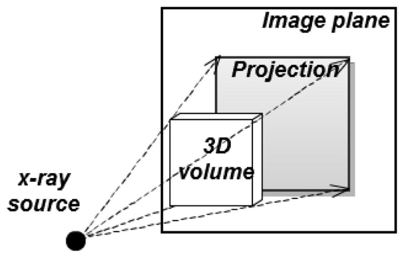
An x-ray projection is simulated by ray-casting on a 3D image volume. The dashed lines and arrows indicate the ray directions.
One way to obtain the estimated parameter updates ΔĈ(t) is by optimizing a measure ρ of the concatenated intensity residue R† with respect to the parameter updates ΔC. The concatenated intensity residues R†, defined as the concatenation over all of the projection angles θ of the residues Rθ: R† = (Rθ1, R θ2,…, R θΓ).
| (2.4) |
Without parallelization, iterative computations to carry out this optimization are structurally slow. Moreover, the optimization may easily converge to a local minimum since the energy functional in eq. 2.4 is not convex. See section 7.2.3 for the detailed evaluation of the optimization-based approach.
2.2. Efficient Linear Approximation of ΔC
We propose an alternative method to calculate ΔC using multi-scale linear operators M. At each iteration of the registration, our method estimates the motion/deformation parameter updates ΔĈ(t) by applying a linear operator Ms of scale s to the current concatenated intensity residue R†. That is,
| (2.5) |
Typically, S = 4 and tmax ≤ 10 are satisfactory. The computation in eq. 2.5 involves only matrix multiplications by Ms, computation of the projections P, and subtractions (eq. 2.2). This makes the registration structurally fast. The calculation of the multi-scale linear operators M involves a machine learning process described in detail in section 4. Due to the leveragable advantage of the machine learning process and the fast linear operation, our proposed method shows a more robust and faster registration than the optimization-based approach. See section 7.2.3 for the comparisons.
3. Shape Space Modeling
Our method limits the motion/deformation to a shape space. To allow M to be accurately learned, we require a low-order parametrization C of this shape space. We describe the shape space calculation for rigid motions and for non-rigid deformations in section 3.1 and 3.2 respectively.
3.1. Rigid Motion Modeling
Rigid motions are modeled explicitly as the variation in the Euler’s six dimensional rigid space:
| (3.1) |
where tx, ty, tz are the translation amounts in cm along the world’s coordinate axes x, y, z, respectively; and rx, ry, rz are the rotations in degrees (°) about the image center, around the world coordinate axes x, y, and z, in succession.
3.2. Deformation Modeling
Like others (Liu et al. [19], Li et al. [9]), we model deformations as a linear combination of a set of basis deformations calculated through principal component analysis (PCA). In our target problem, a cyclically varying set of 3D images {Jτ; over time τ } are available at pre-registration learning time. From these a mean image J̄, and a set of deformations φτ between Jτ and J̄ can be computed. The basis deformations are chosen to be the primary eigenmodes of the PCA of the φτ. The computed mean image J̄ will be used as the reference mean image I throughout this paper.
3.2.1. Deformation Shape Space and Mean Image Generation
In order to model the deformation space realistically, our method computes a Fréchet mean image J̄ via an LDDMM (Large Deformation Diffeomorphic Metric Mapping) framework (Beg et al. [20]) from the cyclically varying set of 3D images {Jτ; over time τ }. The Fréchet mean, as well as the diffeomorphic deformations φ from the mean to each image Jτ, are computed using a fluid-flow distance metric dfluid (Lorenzen et al. [21]):
| (3.2) |
| (3.3) |
where Jτ (x) is the intensity of the pixel at position x in the image Jτ, vτ,γ is the fluid-flow velocity field for the image Jτ in flow time, γ, α is the weighting variable on the image dissimilarity, and φτ (x) describes the deformation at the pixel location .
The mean image J̄ and the deformations φτ are calculated by gradient descent optimization. The set {φτ over τ} can be used to generate the deformation shape space by the following statistical analysis.
3.2.2. Statistical Analysis
Starting with the diffeomorphic deformation set {φτ }, our method uses PCA to find a set of linear deformation basis functions . The scores (basis function weights) for each yield φτ in terms of these basis functions.
| (3.4) |
We choose a subset of n eigenmodes that capture 95% of the total variation. Then we let the n basis function weights λi form the n-dimensional parameterization C.
| (3.5) |
| (3.6) |
4. Machine Learning
From the motion/deformation shape space we calculate linear operators M that correlate coarse-to-fine sampled model parameters C with the corresponding projection intensity residue vectors R. We describe our regression learning to calculate the linear operators M in section 4.1 and an efficient multi-scale learning strategy in section 4.2.
4.1. Residues to Model Parameters Regression Learning
As detailed in section 4.2 we select a collection of model parameters {Cκ over cases κ} for learning. Each case is formed by a selection of parameter settings. The training uses deviations from the reference image, such that ΔC = C κ. Linear regression is used to correlate the selected modeled parameters C in the κth case with the co-varying projection intensity residue set {Rκ,,θ over the projection angles θ}. Rκ θ(x) is computed as the intensity difference at pixel location x = (x1, x2) between the projection at angle θ of the mean image I (or an untransformed 3D image for the rigid case) and the projection of the image I ∘ T (Cκ) transformed with the sampled model parameter Cκ:
| (4.1) |
We concatenate the residues at each projection angle to formulate a residue set in a vector and build a linear regression for all cases κ= 1, 2, …, K:
| (4.2) |
The regression matrix M that gives the best estimation of the linear operators per parameter scale is computed via a pseudo-inverse:
| (4.3) |
4.2. Multi-scale Learning
To provide adequate regression learning, C must be sufficiently sampled to capture all the shape variations. However, the direct implementation requires an exponential time computation. Instead, we have designed an efficient scheme that learns the model parameters from large to small scales, 1 to S, to yield S scale-related regression matrices M1, M2, …, MS. At the σth scale of learning, each model parameter ci is collected from the combinations of ±3σi · (S − σ + 1)/S and 0 where σi is the standard deviation of the basis function weights i observed at pre-registration time. In the registration stage the calculated multi-scale linear operators are applied sequentially, from M1 to MS, to give new estimations of the model parameters from large to small scale. After evaluating the estimation accuracy for target examples of both the rigid and non-rigid types, we found that four scales of learning (S = 4) produced sufficiently dense samples in C to achieve the required registration accuracy.
5. Commensurate Projection Intensity Generation
X-ray scatter is a significant contribution to the cone-beam CT projections. However, the regression estimators M are not invariant to the projection intensity variations caused by x-ray scatter. Therefore, our method uses a normalization filter (section 5.1) and a subsequent histogram matching scheme (section 5.2) to generate commensurate intensities between learning-time computed projections and registration-time target projections.
5.1. Local Gaussian Normalization
To account for variations caused by x-ray scatter, we perform a 2D Gaussian-weighted normalization for each pixel in the learning projections (Figure 5.1 (d)) and the target projections (Figure 5.1 (b)). To calculate the normalized value Ψ′(x;θ) at pixel location x = (x1, x2) and projection angle, θ we subtract a Gaussian-weighted spatial mean μ′ (x1, x2) from the raw pixel value Ψ (x1, x2) and divide it by a Gaussian-weighted standard deviation σ′ (x1, x2).
Figure 5.1.

(a) A raw Cone-Beam CT (CBCT) projection (target projection), (b) a local Gaussian normalized CBCT projection (normalized target projection), (c) histogram matched CBCT projection (normalized and histogram matched target projection) and (d) a local Gaus-sian normalized DRR of a Fréchet mean CT (learning projection) from a lung dataset. As shown in the images, after normalization and histogram matching, the intensity contrast in the target projection becomes closer to that in the learning projection.
| (5.1) |
| (5.2) |
| (5.3) |
where 2A + 1 and 2B + 1, respectively, are the number of columns and rows in the averaging window centered at (x1, x2); the function G is a zero mean Gaussian distribution with a standard deviation w. We choose A, B, and w to be a few pixels to perform a local Gaussian-weighted normalization for our target problem (see section 6).
5.2. Histogram Matching
In order to correct the intensity spectrum differences between the normalized learning projection and the normalized target projection a function Fω of intensity to achieve non-linear cumulative histogram matching within a region of interest ω is applied. To avoid having background pixels in the histogram, the region ω is determined as that pixel set whose intensity values are larger than the mean value in the projection. That is, Fω is defined by
| (5.4) |
where Hf is the cumulative histogram profiling function. The histogram matched intensities (Figure 5.1 (c)) are calculated through the mapping:
| (5.5) |
6. Experimental Setup and Clinical Context
We describe the experimental setups for evaluating the method and provide some clinical context. Our target problem is IGRT (Image-guided Radiation Therapy). There the 3D image I is the planning CT (Computed Tomography), and the target projection images Ψ are treatment-time imaging kV projections. In particular, the kV projections are produced by 1) a rotational CBCT (Cone-beam CT) imager or 2) a stationary NST (Nanotube Stationary Tomosynthesis) imager specified in Maltz et al. [22]. Our method’s application to IGRT, referred to as Correction via Limited-Angle Residues in External Beam Therapy, or CLARET (Chou et al. [14, 15]), has shown promise in registering the planning CT to the treatment-time imaging projections. We describe the two treatment imaging geometries in section 6.1 and CLARET’s application to head-and-neck IGRT and lung IGRT in sections 6.2 and 6.3, respectively.
6.1. Treatment Imaging Geometry
6.1.1. Cone-beam CT (CBCT)
A CBCT is a rotational imaging system with a single radiation source and a planar detector, which are mounted on a medical linear accelerator. This pair rotates by an angle of up to 2π during IGRT, taking projection images Ψ during traversal (Figure 6.1 (a)). A limited-angle rotation provides a shortened imaging time and lowered imaging dose. For example, a 5′ rotation takes ~ 1 second. In our application, CBCT projections were acquired in a half-fan mode. Half-fan mode means that the imaging panel (40 cm width by 30 cm height, source-to-panel distance 150 cm) is laterally offset 16 cm to increase the CBCT reconstruction diameter to 46 cm. The method’s linear operators are trained for projection angles over 360 degrees at 1 degree intervals beforehand at planning time. At treatment time the method chooses the linear operator that is closest to the current projection angle.
Figure 6.1.
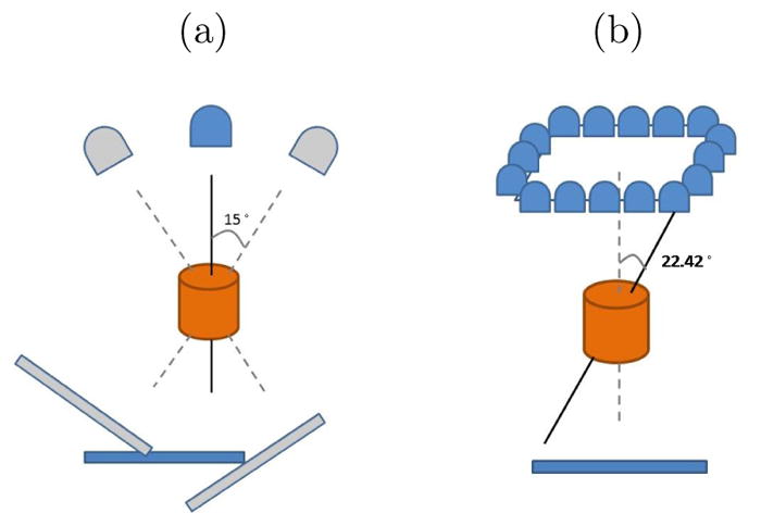
(a) Short arc CBCT geometry: rotational imaging system depicting a 30° arc. The image detector is laterally offset for half-fan acquisition. (b) The NST geometry: stationary sources array with angle θ = 22.42°
6.1.2. Nanotube Stationary Tomosynthesis (NST)
An NST is a stationary imaging system mounted on a medical linear accelerator that can perform imaging without interfering with treatment delivery. As illustrated in Figure 6.1 (b), it consists of an arrangement of radiation sources arrayed around the treatment portal, together with a planar detector. The geometry thus is fixed and known beforehand. Firing the sources in sequence produces a sequence of projection images at different orientations. Each projection image requires ~ 200 ms.
6.2. Head-and-neck IGRT
In head-and-neck IGRT, the geometric differences of the skull between planning time and treatment time can be represented by a rigid transformation. Therefore, in the pre-registration learning, CLARET samples clinically feasible variations (±2 cm, ±5°) in the Euler’s 6-space C to capture the treatment-time patient’s motions. With a single planning CT I of the patient, the computed learning projections P(x, I ∘ T (C);θ) are generated by transformation of the feasible variations T (C) and projection from a given angle θ of the transformed 3D volume I ∘ T (C).
In the registration, CLARET iteratively applies S multi-scale linear operators M1 to MS to estimate the rigid transformation from the 2D intensity residues formed by the difference between the normalized target projections Ψ★ and the normalized projections computed from the currently estimated rigid transformation applied to the planning-time 3D image.
6.3. Lung IGRT
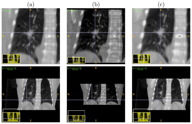
A consideration in lung IGRT is that respiratory motion introduces non-rigid transformations. In the pre-registration learning stage, a set of 10-phase RCCTs (Respiratory-correlated CTs) collected at planning time serve as the cyclically varying 3D images {Jτ over the phase τ }. This image set is used to generate the deformation shape space C. From these RCCTs, a Fréchet mean image J̄ and its deformations φτ to the corresponding images Jτ are calculated via an LDDMM framework. Figure 6.2 (c) shows an example respiratory Fréchet mean image. The deformation basis functions φpc are then generated by PCA on the deformation set {φτ over phase τ }. Liu et al. [19] have shown that a shape space with three eigenmodes adequately captures 95% respiratory variations experienced at treatment time. Figure 6.3 shows the first two principal deformation basis functions.
Figure 6.2.

(a) Respiratory-correlated CT at the End-Expiration (EE) phase (b) RCCT at the End-Inspiration (EI) phase and (c) Fréchet mean CT generated via the Large Deformation Diffeomorphic Metric Mapping framework from the RCCT dataset.
Figure 6.3.
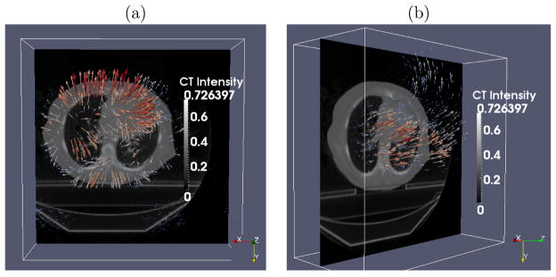
The (a) first and (b) second principal deformation basis functions analyzed from a lung RCCT dataset. Colored lines indicate heated body spectrum presentations of the deformation magnitudes. As shown in the images, the first principal motion consists of anterior-posterior expansion and contraction of the lung, and the second principal motion is along the superior-inferior direction. X⃗: Left to Right (LR); Y⃗: Anterior to Posterior (AP); Z⃗: Superior to Inferior (SI).
To generate feasible variations in the deformation space C for learning the linear operator M, CLARET samples the largest scale of parameters by three standard deviations of the basis function weights derived from the RCCT image set. From the Fréchet mean image the computed projections P(x, I ∘ T (C);θ) are generated by 1) transformation based on the feasible variations T (C) and 2) projection from a given angle θ to the transformed 3D volume I ∘ T (C).
Just prior to treatment, the Fréchet mean image obtained at planning time is rigidly registered to the CBCT for correcting patient position. During treatment with planar imaging, CLARET iteratively applies S multi-scale linear operators, from M1 to MS to estimate the weights C on the basis functions φpc from current 2D intensity residues. The residues are formed by the difference between the normalized and histogram matched target projections Ψ★ (Figure 5.1 (c)) and the normalized projections (Figure 5.1 (d)) computed from the presently estimated deformation applied to the Fréchet mean image.
7. Experiments and Results
We show CLARET’s rigid registration and non-rigid registration results in sections 7.1 and 7.2, respectively. In particular, we tested the rigid registration using the NST imaging system for the head-and-neck IGRT and tested the non-rigid registration using projection images from CBCT scans acquired with the rotational imaging system lung intratreatment IGRT. In section 7.2.3 we compare the registration accuracy and efficiency of CLARET and an optimization-based approach.
7.1. Rigid Registration Results
We tested CLARET’s rigid registration by synthetic treatment-time projections and by real phantom projections, as described in sections 7.1.1 and 7.1.2, respectively. The registration quality was measured by the mean absolute error (MAE) and mean target registration error (mTRE). The MAE in any of the parameters of C is the mean, over the test cases, of the absolute error in that parameter. The mTRE for a test case is the mean displacement error, over all voxels in a 16× 16× 16 cm3 bounding box (the probable tumor region) centered on the pharynx in the planning CT I.
| (7.1) |
where χ is the number of pixels in the probable tumor region, yi = (y1, y2, y3) is the tuple of the ith voxel position, and Ct;rue, Cest; are the true and the estimated transformation parameters, respectively.
7.1.1. Synthetic Treatment Projections
We used noise-added DRRs (digitally reconstructed radiographs) of target CTs as the synthetic treatment-time projections. The DRRs (Figure 7.1(a)) were generated to simulate the NST projections with dimension 128 × 128 and pixel spacing 3.2 mm (Figure 2.1). The target CTs were transformed from the patient’s planning CT by taking normally distributed random samples of the translation and rotation parameters within the clinical extent: ±2 cm and ±5°, respectively. The planning CTs have a voxel size of 1.2 mm lateral, 1.2 mm anterior-posterior, and 3.0 mm superior-inferior. The number of imaging positions was varied to find the minimum number with sub-CT-voxel accuracy in terms of mTRE.
Figure 7.1.
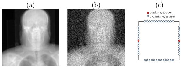
(a) A raw DRR from a x-ray source in the NST (b) DRR with Gaussian noise added (c) the NST geometry of two opposing x-ray sources
Zero mean, constant standard deviation Gaussian noise was added to the DRRs to generate the synthetic projections. The standard deviation of the noise was chosen to be 0.2 × (mean bony intensity - mean soft tissue intensity). This noise level is far higher than that produced in the NST system. An example synthetic projection is shown in Figure 7.1(b).
We first studied how many projection images are needed for CLARET’s learning to obtain sub-voxel accuracy. The results on 30 synthetic test cases of a head-and-neck dataset, displayed in Figure 7.2(a), show that two projection images are sufficient to achieve sub-CT-voxel accuracy. Figure 7.2(a) also shows the method’s accuracy improves with more projections. However, we note that redundant projections may contribute error in the parameter estimation. Therefore, the 4-projection geometry (Figure 7.2(a)), which used the middle x-ray source on each imaging bank, produced the sufficient and necessary number of projections to capture the simulated rigid motions. Figure 7.1(c) shows the geometry of the two opposing x-ray sources that generated the two projection images in the study. We note that the choice of opposing sources is such that the maximum angle between images (22.5 degrees) is formed with the NST system.
Figure 7.2.
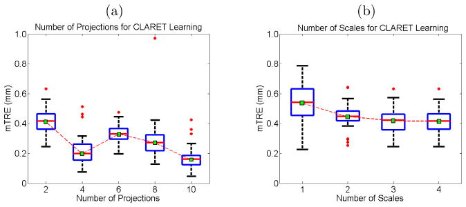
Boxplot results of errors in varying (a) the number of projections used and (b) the number of scales used for CLARET’s rigid registration. Red dots are the outliers. In (a), projections of equally-spaced sources were used.
An analysis of the effect of the number of scales on multi-scale learning (section 4.2) shows that increasing the number of scales reduces the registration errors (Figure 7.2(b)).
Table 1 shows the statistics of the errors in each rigid parameter from 90 synthetic test cases generated from three patients’ planning CTs (30 cases for each CT). The CLARET registration used only the two opposing NST projection images (Figure 7.1(c)).
Table 1.
Mean absolute errors (MAE) and standard deviation (SD) of the absolute errors of the six rigid parameters obtained from 90 synthetic test cases in which CLARET registration used two synthetic NST projection images.
| (mm; °) | Tx | Ty | Tz | Rx | Ry | Rz | mTRE |
|---|---|---|---|---|---|---|---|
| MAE | 0.094 | 0.302 | 0.262 | 0.1489 | 0.0248 | 0.1540 | 0.524 |
| SD | 0.085 | 0.211 | 0.715 | 0.1093 | 0.0174 | 0.2824 | 0.728 |
7.1.2. Real Treatment Projections
We tested CLARET’s rigid registration on a head phantom dataset. NST projections (dimension: 1024 × 1024; pixel spacing: 0.4 mm) of the head phantom were downsampled to dimension 128 × 128 with a pixel spacing of 3.2 mm (Figure 7.3(a)). The dimension of the planning CT is 512 × 512 × 96 with a voxel size of 3.43 mm3. The ground truth was obtained by rigidly registering all 52 NST projections to the planning CT by the l-BFGS optimization (Nocedal [23]) of the similarity metric in projection space.1 The initial mTRE over the head region is 51.8 mm. With 4-scale learning (S = 4), CLARET obtained a sub-voxel accuracy of 3.32 mm using only two projections in 5.81 seconds. It was computed on a 16-core laptop GPU (NVIDIA GeForce 9400m) where the parallelization is limited. A factor of 32 speed-up (0.18 seconds per registration) can be expected when using a 512-core GPU. As shown in Figure 7.3(b) and 7.3(c), CLARET accuracy improves with increased number of projections and scales in the multi-scale learning process. The registration time is approximately linear with the number of projections used.
Figure 7.3.

(a) One of the testing NST projection of a head phantom. (b) Time plots and (c) error plots of CLARET’s registrations on a real head-and-neck phantom dataset. Registrations were accelerated on a 16-core laptop GPU (NVIDIA GeForce 9400m).
7.2. Non-rigid Registration Results
We tested CLARET’s non-rigid registration with synthetic and real patient cone-beam projections, as described in sections 7.2.1 and 7.2.2, respectively. RCCT datasets (CT dimension 512×512×120; voxel size 1 mm lateral × 1 mm anterior-posterior × 2.5 mm superior-inferior) were generated with an 8-slice scanner (LightSpeed, GE Medical Systems) by acquiring multiple CT images for a complete respiratory cycle at each couch position while recording patient respiration (Real-time Position Management System, Varian Medical Systems). The CT projections were retrospectively sorted (GE Advantage 4D) to produce 3D images at 10 different respiratory phases.
7.2.1. Synthetic Treatment Projections
We used DRRs of the target CTs as the synthetic treatment-time projections. The DRRs were generated to simulate projections from a rotating kV imaging system (section 6.1.1) mounted on the gantry of the medical accelerator (TrueBeam, Varian Medical Systems). The target CTs were deformed from the patient’s Fréchet mean CT by taking normally distributed random samples of the coefficients of the first three PCA-derived deformation eigenmodes of the patient’s RCCT dataset (section 3.2).
For each of the 10 CLARET registrations, we used a single simulated coronal projection (dimension 128 × 96; pixel spacing 3.10 mm) at angle 14.18° (Figure 5.1(d)) as input. (Future studies will investigate the effect of this pixel spacing on the registration quality.) The registration quality was then evaluated by measuring the 3D tumor centroid difference between the CLARET-estimated CT and the target CT. 3D tumor centroids were calculated from active contour (geodesic snake) segmentations (Yushkevich et al. [25]). As shown in Table 2, after registration CLARET reduces more than 85% of the centroid error.
Table 2.
3D tumor centroid error (mm) before and after CLARET’s registration for the 10 randomly generated test cases.
| Case # | 1 | 2 | 3 | 4 | 5 | 6 | 7 | 8 | 9 | 10 |
|---|---|---|---|---|---|---|---|---|---|---|
| Before | 8.2 | 21.3 | 21.8 | 20.1 | 9.9 | 10.2 | 10.9 | 15.7 | 14.9 | 19.9 |
| After | 1.3 | 0.8 | 1.5 | 3.3 | 0.8 | 1.3 | 0.5 | 1.6 | 2.1 | 2.7 |
We studied CLARET’s registration quality in terms of average DVF (Displacement Vector Field) error over all cases and all CT voxels versus different angular spacings used in learning. Registrations using two projections with four differ-ent angle separations were tested by 30 randomly generated test cases. Figure 7.4(a) shows that the average DVF error reduces with appropriately large angular separations. However, tumor motion or respiratory motion may not be visible or inferable in projections from certain angles. For example, the tumor may be obscured by denser organs (i.e., mediastinum). In Figure 7.4(a) the respiration motion may not be inferable from the projection at 9.68° resulting in a larger error in the parameter estimation.
Figure 7.4.
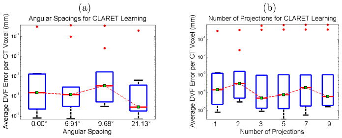
Boxplots of average displacement vector field errors when varying (a) the angular spacing and (b) the number of projections used for CLARET’s non-rigid registration. Red dots are the outliers. In (a), two projections for each test were used. For the zero-degree test case, only one projection was used. In (b), DRRs spanning 9.68° about 14.18° were used in each test. The single projection was tested at 14.18° (see Figure 5.1(d)).
We also studied CLARET’s registration quality by measuring the average DVF error versus the number of projections used for learning. For each number of projections, we generated 30 random test cases. Figure 7.4(b) shows no particular trend. As a result, we used a single projection to test CLARET’s non-rigid registration for the real patient data in the next section.
7.2.2. Real Treatment Projections
We tested CLARET on 5 lung patient datasets consisting of projections from patient CBCT scans acquired with the rotational imaging system (section 6.1.1). CLARET 2D/3D registration used a single coronal CBCT projection at angle 14.18° and downsampled (original dimension 1024 × 768 and pixel spacing 0.388 mm) to 128 × 96 with 3.10 mm pixel spacing (Figure 5.1(a)). Separate registrations were done using projections at the EE (End-Expiration) and EI (End-Inspiration) phases. Prior to 2D/3D registration, the Fréchet mean image was rigidly registered to the patient’s CBCT image so as to align the vetebral anatomy in both images. We measured the difference in 3D tumor centroid position (Figure 7.6(a)) between the CLARET-estimated CT and reconstructed CBCT at the same respiratory phase as the projection used in the 2D/3D registration. The RMS window width was set to 32.0 mm for the Gaussian normalization of this imaging geometry, which was predetermined to yield the smallest 3D centroid error in one lung dataset (Figure 7.5). (Future studies will check whether this window size is also best for other datasets.) The results shown in Table 3 suggest a consistency in registration quality between the synthetic image tests and real projection image tests. The mean and standard deviation of 3D tumor centroid errors following 2D/3D registration are 2.66 mm and 1.04 mm, respectively. The errors include an uncertainty in tumor position in the CBCT projections, owing to variability in the manual segmentations in the CBCT reconstructions, and residual tumor motion within the EE and EI phase intervals. Based on repeatability measurements of the manual segmentations and tumor motion analysis of the RCCT datasets, we estimate the standard deviation uncertainty in manually determined tumor 3D position to be 1 mm. The average computation time is 2.61 seconds on a 128-core GPU, NVIDIA GeForce 9800 GTX. A factor of four speed-up (to 0.65 seconds) can be expected when using a 512-core GPU for acceleration.
Figure 7.6.
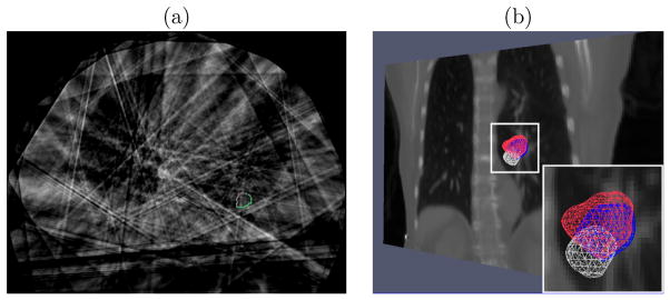
(a) Transaxial image with manual segmented tumor contours in the reconstructed CBCT at one respiratory phase of a lung dataset (patient 3). The contours were used for 3D centroid calculation. (b) Tumor meshes in the Fréchet mean CT (white), in the target CBCT at the EE respiratory phase (blue) and in the CLARET-estimated CT (red) of a lung dataset (patient 2). The background is a coronal slice of the mean CT for illustration. The overlap between the estimated and the target tumor meshes indicates a good registration.
Figure 7.5.
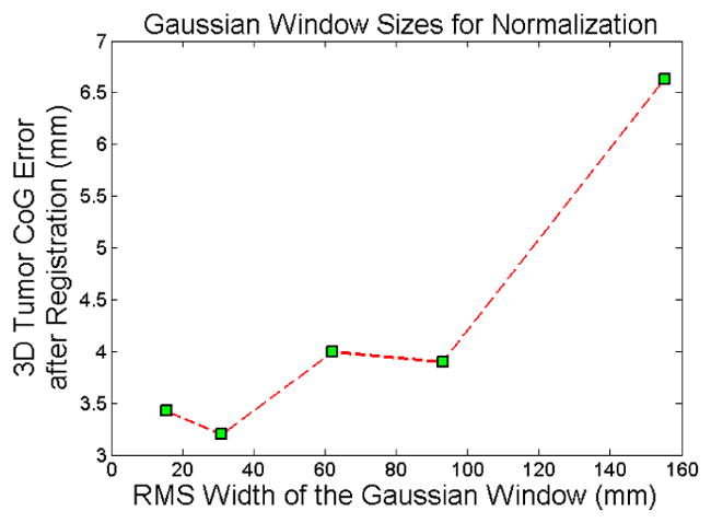
3D tumor centroid error plots on a lung dataset for varying width of the Gaussian window used for CLARET’s local Gaussian normalization.
Table 3.
3D and 2D tumor centroid errors (mm) of EE phase, and ; 3D and 2D tumor centroid errors (mm) of EI phase, and ; computation time for 5 patient datasets. Numbers inside the parentheses are, respectively, the tumor centroid error (mm) before CLARET registration (using Fréchet mean image), and percentage error reduction after registration. The 2D error refers to the tumor centroid error in the directions orthogonal to the projection direction (coronal plane).
| Patient # |
|
|
|
|
Time (s) | ||||
|---|---|---|---|---|---|---|---|---|---|
| 1 | 2.27 (7.96,72%) | 2.07 (4.16,50%) | 5.26 (8.03,34%) | 4.71 (6.80,31%) | 1.94±0.74 | ||||
| 2 | 3.20 (9.70,67%) | 2.23 (9.18,76%) | 2.85 (7.45,62%) | 1.64 (6.77,75%) | 3.99±1.99 | ||||
| 3 | 1.32 (1.47,10%) | 1.32 (1.47,10%) | 2.03 (3.63,44%) | 1.86 (3.49,47%) | 2.45±0.15 | ||||
| 4 | 2.77 (10.17,73%) | 1.51 (9.67,84%) | 2.31 (5.53,58%) | 1.52 (5.17,71%) | 1.96±0.02 | ||||
| 5 | 2.24 (3.52,36%) | 1.91 (3.46,45%) | 2.40 (3.89,38%) | 0.83 (3.16,74%) | 2.76±1.26 |
The clinical goal is to improve tumor localization during treatment using CLARET. Assuming a mean lung tumor motion extent of about 10 mm, the standard deviation uncertainty is about one-third of the motion extent, or 3 mm. In order to improve on current clinical practice (i.e., no image guidance during treatment) a standard deviation uncertainty of 2 mm or less is desirable. Furthermore, since most of the motion is in the inferior-superior direction, it is desirable to achieve 2 mm uncertainty or less in that direction. Our results show that CLARET achieves the clinically desired accuracy: the mean and standard deviation 2D tumor centroid error after registration is 1.96 mm and 1.04 mm, respectively. CLARET reduces positional errors in directions along the plane of the projection more than in the out-of-plane direction. As shown in Table 3, most of the percent 2D error reductions (coronal in-plane), except cases from patient #1, are larger than 3D error reductions. This is expected because 2D/3D registration with a single projection is more sensitive to tumor displacements in the image plane but less sensitive to scale changes due to out-of-plane displacements.
Figure 7.6(b) shows the 3D meshes of the tumors in the Fréchet mean CT, the CBCT at EE, and the estimated CT of a lung dataset for visual validation. As shown in the Figure, the tumor position in the CLARET-estimated CT is superior to that in the mean image, as expected physiologically for the EE phase.
Figure 7.7 shows the same 3-space lines in the mean CT, the reconstructed CBCT at the EE phase and the CLARET-estimated CT of a lung dataset. The intersection of the lines with the tumor centroid in the CBCT are in better agreement with the CLARET-estimated CT than with the mean CT, indicating that CLARET can accurately locate the tumor in the plane of the projection (coronal plane) and further corroborating the results of Table 3.
Figure 7.7.
The same 3-space lines in (a) the mean CT, (b) the reconstructed CBCT at the EE phase and (c) the estimated CT of the same lung dataset used in Figure 7.6 (b). Upper row: lines indicate the tumor centroid in the CBCT at the EE phase; lower row: lines indicate the diaphragm contour in the CBCT at the EE phase.
7.2.3. Comparison to an optimization-based registration method
We compared the registration accuracy and efficiency between CLARET (eq. 2.5) and an optimization-based method similar to that in Li et al. [9]. The optimization-based method we implemented optimizes eq. 2.4 (with ρ = 2) using the l-BFGS quasi-Newton algorithm (Nocedal [23]). To make fair comparisons, we used the same deformation shape space, the same initializations, the same GPU acceleration for the projection operator P, and the same testing datasets. For the comparisons, we randomly sampled 30 synthetic deformations for each of the five lung patients as the test cases. The deformations are sampled randomly within ±3 standard deviations of deformations observed in the patient’s RCCTs. For each test case, a single coronal CBCT projection (dimension: 1024 × 768 downsampled to dimension: 128×96) was simulated from the deformed Fréchet mean CT as the target projection. Both methods were initialized with the realistic Fréchet mean image with no deformation: Ĉ(0) = 0 in eq. 2.1.
For CLARET, we used 4 scales of learning for each patient. At the σth scale of learning, each deformation parameter ci (i = 1, 2, 3) was collected from the combinations of ±3σi · (4 − σ + 1)/4, ±1.5σi · (4 − σ + 1)/4, and 0 where σi is the standard deviation of the ith eigenmode weights observed in the patient’s RCCTs. Therefore, at each scale of learning, 125 training deformations are sampled.
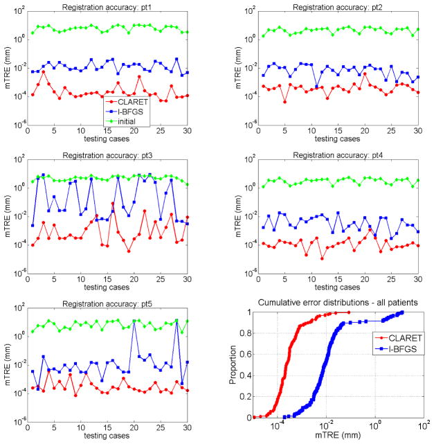
We compare the registration accuracy by the average registration error distance over the lung region. As Figure 7.8 shows, CLARET yields more accurate results than the l-BFGS optimization-based registration in almost every test cases in all five patients. Table 4 shows statistical comparisons of the registration accuracy. The maximum error produced by CLARET among the 30×5=150 test cases is only 0.08 mm where the maximum error produced by l-BFGS is 13.15 mm, which is 164 times higher than CLARET. The smaller median error and error standard deviation also shows that CLARET is more accurate and more robust than the l-BFGS optimization-based approach.
Figure 7.8.
mean target registration error (mTRE) on test data generated from five patients (pt1-pt5): CLARET vs. the l-BFGS optimization vs. the initial error before registration.
Table 4.
Registration accuracy (mTRE) statistics on the five patient data: CLARET vs. the l-BFGS optimization. std=standard deviation
| mTRE (mm) | min. | max. | median | mean | std |
|---|---|---|---|---|---|
| CLARET | 1.1e−5 | 0.08 | 2.3e−4 | 1.5e−3 | 7.4e−3 |
| l-BFGS | 2.0e−4 | 13.15 | 8.8e−3 | 0.54 | 2.01 |
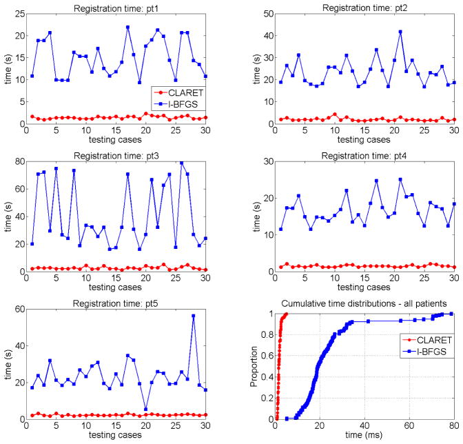
In term of registration speed, Figure 7.9 shows that CLARET is faster than l-BFGS in every test case and has relatively small variation in speed. The statistical results shown in Table 5 indicate that the longest registration time produced by CLARET is still shorter than the shortest time produced by l-BFGS.
Figure 7.9.
Registration time on the five patient data (pt1-pt5): CLARET vs. the l-BFGS optimization.
Table 5.
Registration time statistics on the five patient data: CLARET vs. the l-BFGS optimization. std=standard deviation
| time (s) | min. | max. | median | mean | std |
|---|---|---|---|---|---|
| CLARET | 0.94 | 5.15 | 1.73 | 1.95 | 0.74 |
| l-BFGS | 5.29 | 78.73 | 19.30 | 23.76 | 14.41 |
As our results show, in our implementations CLARET is more robust, accurate, and faster than the l-BFGS optimization.
8. Conclusions and Discussion
We have presented a novel rigid and non-rigid 2D/3D registration method that estimates an image region’s 3D motion/deformation parameters from a small set of 2D projection images of that region. Our clinical goal is to model not only temporal changes in tumor position and shape (tumor tracking), but also those for the surrounding organs at risk. In this context the volume of interest is known to exhibit deformations (Mageras et al. [26], Rosu et al. [27]). The method is based on producing limited-dimension parameterization of geometric transformations based on the region’s 3D images. The method operates via iterative, multi-scale regression, where the regression matrices are learned in a way specific to the 3D image(s) for the specific patient. The synthetic and real image test results have shown the method’s potential to provide fast and accurate tumor localization with a small set of treatment-time imaging projections for IGRT. Faster registration is expected when a modern GPU is used for a higher level of parallelization.
However, in order to obtain such registration accuracy, our method requires a well-modeled motion/deformation shape space that includes all feasible variations of the image region. In many radiation therapy situations for certain parts of the body, collecting the required number of 3D images of the patient to form the well-modeled shape space is not directly obtainable in current therapeutic practice. Future work will investigate the possibility of modeling the shape space through a patient population.
To make our method more robust for the IGRT application, future work will also evaluate the method on more patient datasets and study the effects of the projection resolution and the normalization window size on the registration accuracy.
A novel rigid or deformable 2D/3D image registration method using regression learning.
The method learns a shape space of geometric transformation from the 3D image set.
The method uses multi-scale linear regressions on the 2D image intensity residues.
Target problem is registration between planning time and treatment time in radiotherapy.
Acknowledgments
The authors thank Lei Pan, Dr. Xiaoxiao Liu, and Dr. David Lalush for their fruitful discussions during the development of this work. This work was partially supported by Siemens Medical Solutions and by National Cancer Institute Award Numbers R01-CA126993 and R01-CA126993-02S1. The content is solely the responsibility of the authors and does not necessarily represent the official views of the National Cancer Institute or the National Institutes of Health.
Footnotes
Results in Frederick et al. [24] suggests that 2D/3D registration accuracy is higher than limted-angle-reconstructed-3D/3D registration accuracy for the NST geometry.
Publisher's Disclaimer: This is a PDF file of an unedited manuscript that has been accepted for publication. As a service to our customers we are providing this early version of the manuscript. The manuscript will undergo copyediting, typesetting, and review of the resulting proof before it is published in its final citable form. Please note that during the production process errorsmaybe discovered which could affect the content, and all legal disclaimers that apply to the journal pertain.
References
- 1.Markelj P, Tomazevic D, Likar B, Pernus F. A review of 3D/2D registration methods for image-guided interventions. Medical Image Analysis. 2012;16(3):642–661. doi: 10.1016/j.media.2010.03.005. [DOI] [PubMed] [Google Scholar]
- 2.Russakoff D, Rohlfing T, Maurer C. Fast intensity-based 2D-3D image registration of clinical data using light fields, in: Computer Vision, 2003. Proceedings Ninth IEEE International Conference. 2003;1:416–422. [Google Scholar]
- 3.Russakoff DB, Rohlfing T, Mori K, Rueckert D, Ho A, Adler JR, Maurer CR. Fast generation of digitally reconstructed radiographs using attenuation fields with application to 2D-3D image registration. IEEE Transactions on Medical Imaging. 2005;24:1441–1454. doi: 10.1109/TMI.2005.856749. [DOI] [PubMed] [Google Scholar]
- 4.Khamene A, Bloch P, Wein W, Svatos M, Sauer F. Automatic registration of portal images and volumetric CT for patient positioning in radiation therapy. Medical Image Analysis. 2006;10:96–112. doi: 10.1016/j.media.2005.06.002. [DOI] [PubMed] [Google Scholar]
- 5.Munbodh R, Jaffray DA, Moseley DJ, Chen Z, Knisely JPS, Cathier P, Duncan JS. Automated 2D-3D registration of a radiograph and a cone beam CT using line-segment enhancement. Medical Physics. 2006;33:1398–1411. doi: 10.1118/1.2192621. [DOI] [PMC free article] [PubMed] [Google Scholar]
- 6.Furtado H, Gendrin C, Bloch C, Spoerk J, Pawiro SA, Weber C, Figl M, Stock M, Georg D, Bergmann H, Birkfellner W. Real-time 2D/3D registration for tumor motion tracking during radiotherapy. Proc SPIE 8314, Medical Imaging 2012: Image Processing. 2012;8314:831407. doi: 10.1117/12.910117. [DOI] [Google Scholar]
- 7.Gendrin C, Furtado H, Weber C, Bloch C, Figl M, Pawiro SA, Bergmann H, Stock M, Fichtinger G, Georg D, Birkfellner W. Monitoring tumor motion by real time 2D/3D registration during radiotherapy. Radiotherapy and oncology. 2012;102:274–280. doi: 10.1016/j.radonc.2011.07.031. [DOI] [PMC free article] [PubMed] [Google Scholar]
- 8.Li R, Jia X, Lewis JH, Gu X, Folkerts M, Men C, Jiang SB. Real-time volumetric image reconstruction and 3D tumor localization based on a single x-ray projection image for lung cancer radiotherapy. Medical Physics. 2010;37:2822–2826. doi: 10.1118/1.3426002. [DOI] [PubMed] [Google Scholar]
- 9.Li R, Lewis JH, Jia X, Gu X, Folkerts M, Men C, Song WY, Jiang SB. 3D tumor localization through real-time volumetric x-ray imaging for lung cancer radiotherapy. Medical Physics. 2011;38:2783–2794. doi: 10.1118/1.3582693. [DOI] [PubMed] [Google Scholar]
- 10.Banks S, Hodge W. Accurate measurement of three-dimensional knee replacement kinematics using single-plane fluoroscopy. Biomedical Engineering, IEEE Transactions on. 1996;43(6):638–649. doi: 10.1109/10.495283. [DOI] [PubMed] [Google Scholar]
- 11.Freire L, Gouveia A, Godinho F. FMRI 3D registration based on Fourier space subsets using neural networks. Engineering in Medicine and Biology Society (EMBC), 2010 Annual International Conference of the IEEE. 2010:5624–5627. doi: 10.1109/IEMBS.2010.5628038. [DOI] [PubMed] [Google Scholar]
- 12.Zhang J, Ge Y, Ong SH, Chui CK, Teoh SH, Yan CH. Rapid surface registration of 3D volumes using a neural network approach. Image Vision Comput. 2008;26(2):201–210. doi: 10.1016/j.imavis.2007.04.003. URL http://dx.doi.org/10.1016/j.imavis.2007.04.003. [DOI] [Google Scholar]
- 13.Wachowiak M, Smolikova R, Zurada J, Elmaghraby A. A supervised learning approach to landmark-based elastic biomedical image registration and interpolation. Neural Networks, 2002 IJCNN ’02. Proceedings of the 2002 International Joint Conference. 2002;2:1625–1630. doi: 10.1109/IJCNN.2002.1007761. [DOI] [Google Scholar]
- 14.Chou C-R, Frederick C, Chang S, Pizer S. Brain, Body and Machine, vol. 83 of Advances in Soft Computing. Springer; Berlin/Heidelberg: 2010. A Learning-Based Patient Repositioning Method from Limited-Angle Projections; pp. 83–94. [DOI] [Google Scholar]
- 15.Chou C-R, Frederick B, Liu X, Mageras G, Chang S, Pizer S. CLARET: A Fast Deformable Registration Method Applied to Lung Radiation Therapy. Fourth International (MICCAI) Workshop on Pulmonary Image Analysis. 2011:113–124. [Google Scholar]
- 16.Steininger P, Neuner M, Fritscher K, Sedlmayer F, Deutschmann H. A novel class of machine-learning-driven real-time 2D/3D tracking methods: texture model registration (TMR) Proc. SPIE 7964, Medical Imaging 2011: Visualization, Image-Guided Procedures, and Modeling. 2011;7964:79640G. doi: 10.1117/12.878147. [DOI] [Google Scholar]
- 17.Cootes TF, Edwards GJ, Taylor CJ. Active appearance models. IEEE Transactions on Pattern Analysis and Machine Intelligence. 2001;23(6):681–685. [Google Scholar]
- 18.Jurie F, Dhome M. Hyperplane Approximation for Template Matching. IEEE Transactions on Pattern Analysis and Machine Intelligence. 2002;24:996–1000. [Google Scholar]
- 19.Liu X, Davis B, Niethammer M, Pizer S, Mageras G. Prediction-driven Respiratory Motion Atlas Formation for 4D Image- guided Radiation Therapy in Lung. MICCAI’10 Pulmonary Image Analysis Workshop. 2010 [Google Scholar]
- 20.Beg MF, Miller MI, Trouve A, Younes L. Computing Large Deformation Metric Mappings via Geodesic Flows of Diffeomorphisms. International Journal of Computer Vision. 2005;61:139–157. [Google Scholar]
- 21.Lorenzen P, Prastawa M, Davis B, Gerig G, Bullitt E, Joshi S. MultiModal Image Set Registration and Atlas Formation. Medical Image Analysis. 2006;10(3):440–451. doi: 10.1016/j.media.2005.03.002. [DOI] [PMC free article] [PubMed] [Google Scholar]
- 22.Maltz JS, Sprenger F, Fuerst J, Paidi A, Fadler F, Bani-Hashemi AR. Fixed gantry tomosynthesis system for radiation therapy image guidance based on a multiple source x-ray tube with carbon nanotube cathodes. Medical Physics. 2009;36:1624–1636. doi: 10.1118/1.3110067. [DOI] [PubMed] [Google Scholar]
- 23.Nocedal J. Updating Quasi-Newton Matrices with Limited Storage. Mathematics of Computation. 1980;35:773–782. [Google Scholar]
- 24.Frederick B, Lalush D, Chang S. TH-C-201C-10: Registration Using Nanotube Stationary Tomosynthesis: Comparison of 3D/3D to 3D/2D Methods. Medical Physics. 2010;37:3460. doi: 10.1118/1.3469515.. [DOI] [Google Scholar]
- 25.Yushkevich PA, Piven J, Cody Hazlett H, Gimpel Smith R, Ho S, Gee JC, Gerig G. User-Guided 3D Active Contour Segmentation of Anatomical Structures: Significantly Improved Efficiency and Reliability. Neuroim-age. 2006;31(3):1116–1128. doi: 10.1016/j.neuroimage.2006.01.015. [DOI] [PubMed] [Google Scholar]
- 26.Mageras G, Pevsner A, Yorke E, Rosenzweig K, Ford E, Hertanto A, Larson S, Lovelock D, Erdi Y, Nehmeh S, Humm J, Ling C. Measurement of lung tumor motion using respiration-correlated CT. International Journal of Radiation Oncology*Biology*Physics. 2004;60:933–941. doi: 10.1016/j.ijrobp.2004.06.021. [DOI] [PubMed] [Google Scholar]
- 27.Rosu M, Chetty IJ, Balter JM, Kessler ML, McShan DL, Haken RKT. Dose reconstruction in deforming lung anatomy: Dose grid size effects and clinical implications. Medical Physics. 2005;32:2487–2495. doi: 10.1118/1.1949749. [DOI] [PubMed] [Google Scholar]


