MRI Non-Uniformity Correction Through Interleaved Bias Estimation and B-Spline Deformation with a Template

Abstract

We propose a template-based method for correcting field inhomogeneity biases in magnetic resonance images (MRI) of the human brain. At each algorithm iteration, the update of a B-spline deformation between an unbiased template image and the subject image is interleaved with estimation of a bias field based on the current template-to-image alignment. The bias field is modeled using a spatially smooth thin-plate spline interpolation based on ratios of local image patch intensity means between the deformed template and subject images. This is used to iteratively correct subject image intensities which are then used to improve the template-to-image deformation. Experiments on synthetic and real data sets of images with and without Alzheimer’s disease suggest that the approach may have advantages over the popular N3 technique for modeling bias fields and narrowing intensity ranges of gray matter, white matter, and cerebrospinal fluid. This bias field correction method has the potential to be more accurate than correction schemes based solely on intrinsic image properties or hypothetical image intensity distributions.

I. INTRODUCTION

The validity of structural brain MRI studies depends crucially on identifying anatomical correspondences across subjects. MRI images unfortunately contain slowly-varying field non-uniformities that complicate this task by introducing substantial variability in the intensities of pixels from the same tissue class. For this reason, a large literature is devoted to MRI non-uniformity correction. Two broad categories of approaches exist: intrinsic approaches use a priori assumptions of intensity variability within and between tissue classes to correct intensities based solely on the input image provided; relative approaches estimate the bias field by comparing intensities between corresponding locations in subject and reference images. The widely used N3 method [1] is an example of the intrinsic approach. N3 performed well in a survey of six algorithms for non-uniformity correction [2]. Yet methods such as this have potential drawbacks based on their assuming a discrete set of tissue classes and a corresponding intensity histogram exhibiting distinct sharp tissue intensity peaks. Structures like the thalamus and putamen, for example, do not fit into this framework; their intensities typically lie between those of cortical gray matter and subcortical white matter and may be inaccurately represented using this approach.

One example of the relative approach estimates relative bias from ratios of intensities of voxels from like tissues in longitudinal (and therefore anatomically similar) image pairs [3]. In this method longitudinal images are corrected against each other to facilitate computation of brain change over time; there is not a notion of actual bias removal. Another relative method does aim for bias removal. It uses a B-spline deformation to identify correspondences between a subject image and a bias-minimized template. Intensity ratios between these two images are then taken to represent non-uniformities at each subject voxel [4].

Relative methods require good anatomical matching between images to ensure that the ratios of corresponding voxel intensities are valid estimates of differences or actual field nonuniformities. However, the field non-uniformity itself can create difficulties for accurate anatomical matching. Furthermore, inter-individual differences in brain morphology make perfect anatomical matching impossible, and the inevitable tissue mismatches contribute to inaccurate non-uniformity estimates. Finally, image noise is a third component that confounds these estimates. Thus, estimating the non-uniformity field using voxel intensity ratios after completion of a deformation [4] could risk errors due to both poor deformation estimation and unavoidable voxel-level mismatches.

We propose a relative method that overcomes these problems by updating a smoothly-varying multiplicative nonuniformity field model, and correcting the subject image, at each iteration of a B-spline deformation between subject and template. The non-uniformity field is estimated by comparing the summary intensity statistics of extended image patches, rather than comparing intensities between individual voxels, to increase robustness against noise and anatomical mismatch. Non-uniformity field estimates are defined at the centroids of the image patches and interpolated across the brain using 3D thin-plate splines [5]. The resulting reciprocal field corrects the subject image intensities before the next iteration of the deformation. This creates a “bootstrap” process in which an improved deformation yields an improved non-uniformity field estimate, which then yields an improved deformation, and so on.

We hypothesize that such a model, based on comparisons of corresponding local regions, will be relatively insensitive both to local noise and anatomical mismatches. When used with a bias-free template, it should better represent and correct slowly varying nonuniformity fields in structural MRIs.

II. METHODS

A. Overview of the method

We assume that the subject image Y that we observe is the result of superimposing a smooth, slowly varying, multiplicative MRI non-uniformity field R onto a true, underlying subject image I, and that R can be modeled by a thin-plate spline field interpolated from relatively few discrete local measurements. Thus at each voxel x we have

$$Y\left(\mathit{x}\right)=R\left(\mathit{x}\right)I\left(\mathit{x}\right)+E,$$ (1)

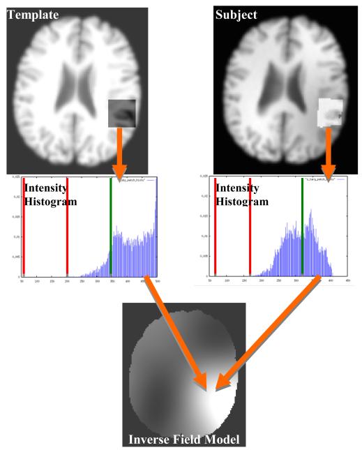
with E is zero-mean Gaussian noise. We use a deformed bias-free template image to approximate I and construct a function R which, when multiplied with our estimate of I, closely approximates Y. R is generated by taking the ratio of intensity summary measures between corresponding image patches in the deformed template and subject images—the patches consist of the image sub-volumes delineated by sets of adjacent B-spline control points as illustrated in Fig. 1. We correct the image at each iteration by multiplying the observed intensity Y(x) by 1/R(x).

Figure 1.

Schematic overview of algorithm. Top row: One patch on the template image (left) corresponds to one deformed patch on the subject image (right). Middle row: The voxel intensity histograms of the patches are divided into sub-ranges (vertical lines) and the mean of the most representative sub-range of each (to right of green divider) is calculated; this sub-range represents the white matter in both patches. Bottom row: the ratio of these two means is used to define the multiplicative reciprocal nonuniformity ratios at discrete single points in the subject image, which are then interpolated over the rest of the volume using thin plate splines to form the inverse field model.

Prior to non-uniformity correction, we smooth the subject image slightly using a 3D Gaussian convolution filter (2.4 mm FWHM), normalize both images to have the same global intensity means, and internally rescale the intensity range to 0 – 500. We then use an affine registration technique using cross correlation as a similarity measure and axis-parallel Brent’s method for optimization to linearly align the template to the subject. Empirically, this step provides a rough alignment that enables accurate B-spline warping, even in the case of severe MRI nonuniformities.

B. Cubic B-spline image warping

We use cubic B-spline warping to deform the template to the subject [6]. We define a 3D control point grid over the template image and deform template image voxel locations by moving the control points. This deformation is performed in a multi-resolution control point hierarchy [7] with three degrees of control point separation: 24 mm, 12mm, and 6mm. At each level in the hierarchy, we define a set of image patches, each of which cover the image sub-volume bounded by a set of adjacent control points on the template image. These image patches are deformed based on the control point motion and thus have a corresponding, deformed image patch defined on the subject image.

C. Computing the intensity ratios at locations defined by lattice points

During the warp, the control grid points of the cubic B-spline warp provide a partitioning of the subject and template images into sub-volumes. Each sub-volume in the template corresponds to a deformed sub-volume in the subject. Using these image patches to tile each image gives paired regions in subject and template over which we estimate voxel intensity ratios. These ratios, assigned to centroids of the deformed patches, are the anchors for the thin-plate spline interpolation of the nonuniformity field.

For the intensity ratio at a given patch, we compute the intensity histogram of the patch in the template and the corresponding patch in the subject (see Fig.1, top and middle rows). For robustness against noise and tissue mismatch, we partition the intensity range of each patch into four subranges, with divisions at 12%, 40%, and 70% of the intensity maximum for the patch. Because the lowest subrange usually corresponds to CSF and is generally not informative for nonuniformity correction, it is discarded. Among the other subranges, the one that represents the largest number of voxels in the template and subject images together is considered the most representative subrange. The average intensity of the representative subrange is computed and the ratio of this average between template and subject is assigned to the centroid of the deformed subject patch (See Fig. 1).

To complete the computation of the bias correction field, the template volume is tiled by sub-volumes of the kind shown on the top left in Fig. 1, and the object image is covered by their deformations. This leads to a set of intensity ratio estimates assigned to a discrete grid of locations within the subject image at the centroids of the deformed cubes. The bias correction ratio field is computed by 3D thin-plate spline interpolation of those point estimates. Thin-plate spline interpolation uses cubic polynomials and the log function [5] to produce a second order differentiable field F(x) that matches the intensity ratios at the sampled locations. The intention is that the interpolated field will avoid local inaccuracies due to noise or tissue mismatch that might result from computing ratios at every voxel, even after smoothing as in [4], while being accurate to the overall non-uniformity field because of robust estimation in each patch. An example of the reciprocal field is illustrated in Fig. 1c.

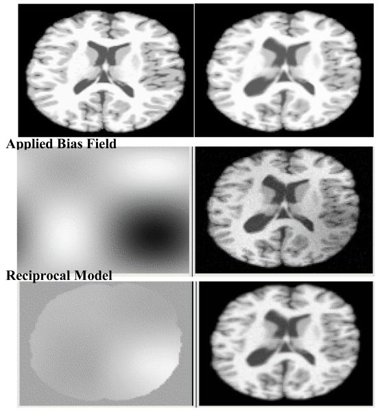
To summarize, when the template image is unbiased, the interpolated ratio field F(x) is an estimate of the reciprocal of the bias on the subject. Therefore multiplication of the subject image by F(x) at each voxel corrects the image. This is illustrated in Fig. 2.

Figure 2.

Top row: MNI phantom brain (left) and distorted image used as subject (right). Middle row: Applied synthetic sinusoidal nonuniformity field (left) and resulting biased brain image (right). Bottom row: Computed reciprocal field used for correction (left) and corrected subject (right).

III. RESULTS

In this section we present results from experiments with phantom and real images to demonstrate the effectiveness of the template-based non-uniformity correction method.

A. Correction of phantom data

We used the bias and noise-free MNI brain phantom (http://www.bic.mni.mcgill.ca/brainweb/selection_normal.html) [8] as the template for the phantom data experiments. To simulate a realistic MRI correction problem, a subject image was created by thin-plate spline deformation of the MNI phantom using manually-displaced landmarks. MRI field non-uniformities were synthesized by multiplying the subject image with a synthetic multiplicative sinusoidal nonuniformity field [2]. Finally we added Gaussian noise with a standard deviation of 3% of maximum white matter intensity, in accordance with the bias and noise model of (1).

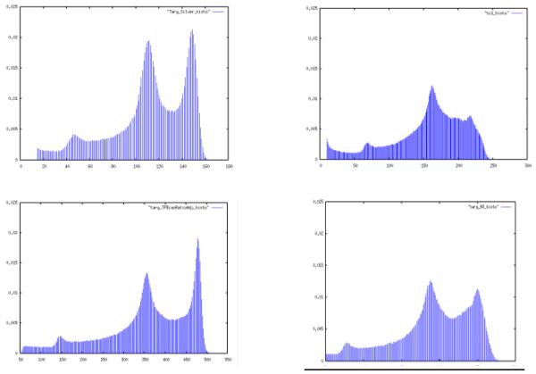
We used our method to correct this subject image, taking the original MNI image as bias-free template (Fig. 2). The template-based method accurately captured the true reciprocal non-uniformity field, leading to a corrected image that lacked any highly visible non-uniformities. We also corrected the same image using N3 [1]. Fig. 3 shows the histograms of the images before and after correction by both methods. The template-based method produced an output image whose intensity histogram peaks more closely resemble the original histogram than N3 did. In particular it has similar relative magnitudes of white and gray peaks, suggesting more faithful tissue class reconstruction. Because each histogram peak corresponds to one tissue class, this result suggests that the template-based method may do a superior job of producing output images that force all pixels within any given tissue class to have intensities within a narrow range, as would be expected in a bias-free image.

Figure 3.

Histograms of bias-free subject (upper left), subject with nonuniformities (upper right), biased subject corrected by template method (lower left) and N3 (lower right). The template method did a better job of restoring the histogram to that of the unbiased image.

B. Correction of real image data

Next we used visual validity and statistical metrics to evaluate our method on real images for which the ground-truth nonuniformity field is not known. We created a minimal deformation image (MDT) [9] based on 29 normal elderly T1-weighted brain MRI images. Then we used this to create a bias-free template by warping the same 29 subjects to the MDT and averaging the resulting images, under the assumption that this would cancel out the nonuniformities present in the individual native images. All MPRAGE images were skullstripped and then linearly aligned to the MDT prior to warp, both for template creation and subsequent experiments in nonuniformity correction.

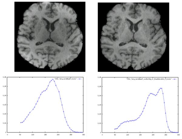
Using the bias-free template we first applied our algorithm to an image with a clearly visible nonuniformity, evaluating the nonuniformity correction by visual inspection of the corrected image and the intensity histogram. Fig. 4 shows sample MRI slices and image intensity histograms before and after correction. Bias seen as darkening of the thalamus, internal capsule, striatum and putamen, and a bright rim near the left posterior cortex (Fig. 4, top left), are visibly corrected. The delineations of caudate, internal capsule and putamen are made clear as darkened gray and white are increased (Fig. 4, top right). Elevated gray intensities such as posterior occipital cortex are similarly reduced. The histograms in Fig. 4 (bottom row), show that gray and white mean intensities are multiplied upward and the tissues separated into distinct peaks. Thus the nonuniformity correction has reduced the variability of tissue intensity within these tissue classes. An expected distinct left “tail” for CSF now appears as well (Fig. 4, bottom right). These features are all missing from the uncorrected image histogram.

Figure 4.

Top row: MRI image before bias correction (left) and after (right). Subcortical structures are much clearer after correction. Bottom row: Intensity histograms before correction (left) and after (right).

Our second experiment used the method to correct nonuniformities from images in a group of cognitively normal elders (CN, N=23) and elders clinically diagnosed with Alzheimer’s disease (AD, N=23). The AD group was expected to be more challenging due to greater morphological variability resulting from the disease. We computed average coefficients of variation (CV) over each group for gray and white tissue types before and after correction. CV is defined as follows [10]:

$$\mathrm{CV}=\sigma ∕\mu ,$$ (2)

where σ and μ are the relevant tissue standard deviation and mean, respectively. CV of image tissue is increased due to tissue nonuniformities; a reduction in CV is one measure of the quality of correction.

To compute the tissue class CV values, we segmented the images (before and after correction) using an EM-based MRF segmentation algorithm due to Rajapakse et al. [11] and used the resulting tissue masks to calculate means and standard deviations of voxel intensities within each class. Table I shows the CV values. As suggested by the example image of Fig. 4, the CV changes were due principally to decreased gray variance. Thus while white tissue CV values were already low due to high mean intensities, gray average CV was reduced by about 25% in each group due to local intensity increase or decrease as appropriate. Therefore the correction method reduced the intensity variability within tissue classes.

Table I.

CV Tissue Values

		Uncorrected	Corrected
AD	G	0.403	0.306
	W	0.138	0.132
CN	G	0.422	0.303
	W	0.134	0.125

IV. CONCLUSION

We have presented an effective and easy to use template-based nonuniformity correction that assumes nothing except a smooth slowly varying nonuniformity field. It performed well on real data and better than N3 at restoring the intensity histogram in phantom data. It should prove a useful tool in nonuniformity correction of 3D structural MRI images.

REFERENCES

- [1].Sled JG, et al. A Nonparametric Method for Automatic Correction of Intensity Nonuniformity in MRI Data. IEEE Transactions on Medical Imaging. 1998;17:87–97. doi: 10.1109/42.668698. [DOI] [PubMed] [Google Scholar]
- [2].Arnold JB, et al. Qualitative and Quantitative Evaluation of Six Algorithms for Correcting Intensity Nonuniformity Effects. NeuroImage. 2001;13:931–943. doi: 10.1006/nimg.2001.0756. [DOI] [PubMed] [Google Scholar]
- [3].Lewis EB, Fox N. Correction of differential intensity inhomogeneity in longitudinal MR images. NeuroImage. 2004;23:75–83. doi: 10.1016/j.neuroimage.2004.04.030. [DOI] [PubMed] [Google Scholar]
- [4].Studholme C, et al. Accurate Template-Based Correction of Brain MRI Intensity Distortion With Application to Dementia and Aging. IEEE Transactions on Medical Imaging. 2004 Jan;23:99–110. doi: 10.1109/TMI.2003.820029. 2004. [DOI] [PMC free article] [PubMed] [Google Scholar]
- [5].Bookstein FL. Shape and the Information in Medical Images: A Decade of Morphometric Synthesis. Computer Vision and Image Understanding. 1997 May;66:97–118. [Google Scholar]
- [6].Rueckert D, et al. Nonrigid registration using free-form deformations: applications to breast MR images. IEEE Transactions on Medical Imaging. 1999;18:712–720. doi: 10.1109/42.796284. [DOI] [PubMed] [Google Scholar]
- [7].Otte M. Elastic Registration of fMRI Data Using Bezier-Spline Transformations. IEEE Transactions on Medical Imaging. 2001 Feb;20:193–206. doi: 10.1109/42.918470. [DOI] [PubMed] [Google Scholar]
- [8].Collins DL, et al. Design and Construction of a Realistic Digital Brain Phantom. IEEE Transactions on Medical Imaging. 1998 Jun;17:463–468. doi: 10.1109/42.712135. [DOI] [PubMed] [Google Scholar]
- [9].Kochunov P, et al. Regional Spatial Normalization: Toward and Optimal Target. Journal of Computer Assisted Tomography. 2001;25:805–816. doi: 10.1097/00004728-200109000-00023. [DOI] [PubMed] [Google Scholar]
- [10].Likar B, et al. Retrospective Correction of MR Intensity Inhomogeneity by Information Minimization. IEEE Transactions on Medical Imaging. 2001 Dec;20:1398–1410. doi: 10.1109/42.974934. [DOI] [PubMed] [Google Scholar]
- [11].Rajapakse JC, et al. Statistical Approach to Segmentation of Single-Channel Cerebral MR Images. IEEE Transactions on Medical Imaging. 1997 Apr;16:176–186. doi: 10.1109/42.563663. [DOI] [PubMed] [Google Scholar]