Retinotopic maps in the pulvinar of bush baby (Otolemur garnettii)

Abstract

Despite its anatomical prominence, the function of primate pulvinar is poorly understood. A few electrophysiological studies in simian primates have investigated the functional organization of pulvinar by examining visuotopic maps. Multiple visuotopic maps have been found in all studied simians, with differences in organization reported between New and Old World simians. Given that prosimians are considered closer to the common ancestors of New and Old World primates, we investigated the visuotopic organization of pulvinar in the prosimian bush baby (Otolemur garnettii). Single electrode extracellular recording was used to find the retinotopic maps in the lateral (PL) and inferior (PI) pulvinar. Based on recordings across cases a 3D model of the map was constructed. From sections stained for Nissl bodies, myelin, acetylcholinesterase, calbindin or cytochrome oxidase, we identified three PI chemoarchitectonic subdivisions, lateral central (PIcl), medial central (PIcm) and medial (PIm) inferior pulvinar. Two major retinotopic maps were identified that cover PL and PIcl, the dorsal one in dorsal PL and the ventral one in PIcl and ventral PL. Both maps represent the central vision at the posterior end of the border between the maps, the upper visual field in the lateral half and the lower visual field in the medial half. They share many features with the maps reported in the pulvinar of simians, including location in pulvinar and the representation of the upper-lower and central-peripheral visual field axes. The second order representation in the lateral map and a laminar organization are likely features specific to Old World simians.

Introduction

The primate pulvinar is located at the dorsal posterior end of the thalamus and at least three subdivisions, or equivalent areas (Gattass et al., 1978), of the pulvinar can be identified: the inferior (PI), lateral (PL), and medial pulvinar (PM) (Walker, 1938, P.48-56; Emmers et al., 1963; Huerta et al., 1986; Wong et al., 2009). Most cells recorded in PL and PI were found to respond to simple visual stimuli (Bender, 1982; Petersen et al., 1985). PI and PL enjoy rich connections with the superior colliculus (SC), the parabigeminal nucleus and the primary visual cortex, as well as other early visual cortical areas of both the dorsal and ventral streams (Kaas & Lyon, 2007). Many functional roles have been proposed for these visual pulvinar subdivisions , including visual salience (Petersen et al., 1987), attention (Van Essen, 2005), visual stability (Robinson & Petersen, 1985; Berman & Wurtz, 2011), motion integration (Merabet et al., 1998), temporal binding (Arend et al., 2008) and as a relay between cortical visual areas (Sherman, 2007; Theyel et al., 2010), among others.

The number and organization of retinotopic maps in the visual pulvinar are of great interest because of pulvinar's wide connections with visual cortical areas and its various proposed functions. The visual pulvinar has been electrophysiologically surveyed in the Old World simian macaque (Bender, 1981) and the New World simian cebus (Gattass et al., 1978). Two retinotopic maps were identified in both species. However, the positions and visual field representations of these maps were reported to differ. In macaque, one map was reported in ventro-lateral PL and the other was described as straddling the PI/PL border (Bender, 1981), while one was found in ventral PI/PL and the other in dorsal PL in cebus (Gattass et al., 1978). The relationship between these observed pulvinar maps in macaque and cebus monkeys remains unclear: 1) the positions of homologous retinotopic maps may have shifted between Old World and New World simian species, 2) true differences between the reported maps may have developed between the species, or 3) maps may not have been detected in the study of one of these species.

Compared to simians, prosimians are considered to be closer to the common ancestors of modern primates (Jerison, 1979) and generally have smaller and less differentiated pulvinar compared to simians (Raczkowski & Diamond, 1981) With knowledge of pulvinar retinotopy of a prosimian, the comparison between it and that of simians can help reveal the following: the common structure of primate pulvinar, the correspondence between reported pulvinar retinotopic maps in different primate species, and potentially, pulvinar features that have evolved solely in simians. Additionally, the functional features of simian pulvinar that are recently evolved are likely to have evolved separately for New and Old World simians, and may correlate with simians’ expanded development of extrastriate cortex. The retinotopic organization of pulvinar, however, has not been electrophysiologically examined in any prosimian species. In this study we used bush babies (Otolemur garnettii) as a representative species of prosimians. We electrophysiologically examined the retinotopy of its visual pulvinar and constructed 3D models of the maps from data across cases. We also compared the resulting functional maps with the chemoarchitecture of each pulvinar subdivision.

Materials and Methods

Animal Preparation

Six bush babies (Otolemur garnettii) of both sexes weighing 0.77-1.1 kg were used in this study. All experiments were performed according to a protocol approved by the Vanderbilt University Institutional Animal Care and Use Committee (IACUC). Some of these animals were used in multi-day terminal recording sessions while others underwent a series of 1-day survival recording sessions before a final 1-day terminal recording session.

Anesthesia was first induced with 20-40 mg/kg ketamine and 0.4-0.5 mg/kg xylazine, and maintained with 1-3% isoflurane during surgery. During the first session a 8 mm craniotomy and durotomy were performed over LGN at the Horsley-Clarke coordinates of anterior-posterior +3 and medial-lateral 7. After surgery, isoflurane was replaced by urethane in terminal sessions and propofol/nitrous oxide in survival sessions. Urethane was given intra-peritoneally, induced with a dose of 1.25 mg/kg and maintained with 0.25 mg/kg boosters every 2 hours. For propofol/nitrous oxide anesthesia, the animal was given propofol intra-venously at 2.5-6 mg/kg/hr first and then at 0.2-0.6 mg/kg/hr after the animal was stabilized. Once the animal was deeply anesthetized, it was given the muscle relaxant, vecuronium bromide, intravenously at 0.15 mg/kg/hr. While the animal was infused with vecuronium bromide, it was respired with 75% nitrous oxide in oxygen in the survival sessions, or room air in the terminal sessions. During the recording session the end tidal CO2 pressure was monitored and maintained between 35 and 50 mmHg. EEG and ECG were monitored to ensure a stable anesthetic plane, and the animals’ toes were pinched periodically to help with ECG monitoring of anesthesia.

The animals pupils were dilated with 1% topical atropine solution. The eyes were focused onto a tangent screen 57 cm away using contact lenses of appropriate size and power. A map of the blood vessel pattern was reflected back on to the tangent screen from the tapetum to locate the optic disks, which were used to infer the locations of the area centralae.

A survival recording session usually lasted 10-12 hours, after which the brain opening was covered with tecoflex (artificial dura) for protection. A specially molded plastic cap of appropriate size was glued with dental cement over the craniotomy window, and the scalp was sutured closed. First vecuronium bromide infusion and then propofol anesthesia was withdrawn and the animal was monitored until it was fully awake, at which point it was given treats and the analgesic buprenorphine 0.01 mg/kg. After a survival session an animal was allowed at least two weeks to recover before another survival session was performed. All pulvinar mapping was done on the left hemisphere. Some of these animals received tracer injections in the right pulvinar for a related study.

Recording

We recorded extracellular single and multi-unit activity using epoxylite-coated tungsten microelectrodes (FHC Inc., Bowdoin, ME) with impedances ranging from 1 to 2.5 ^Ω at 1 kHz. The signal was amplified and digitized with a Plexon multichannel acquisition processor (Plexon Inc., Dallas, TX), and fed to a speaker after filtering. The high impedance of these electrodes ensured that we could differentiate between background hash and neural spikes.

The central vision representation of bush baby pulvinar was found by first looking for the central vision representation of LGN near the Horsley-Clarke coordinates of AP +3 and ML 7, and then moving 1.5 to 2 mm medially. The electrode was initially lowered 7-7.5mm from the cortical surface, then advanced in steps of 100 ^μm. At each location, we examined the visual responsiveness of cells using spots, bars and other light patterns projected on the tangent screen. At peripheral locations we used a hand held screen to roughly estimate the receptive field locations off-screen.

When we found any visual response with bright light spots, we used an ophthalmoscope to project confined light spots or light bars with clear borders and uniform luminance on the screen, to locate the receptive field. Recorded units were classified as vague, moderate or brisk by their visual responses. A brisk unit showed large clear spikes and a clear response similar to the response of V1 cells, with either no adaptation or fast recovery. A moderate unit showed a clear receptive field, spikes clearly larger than background hash and consistent recovery from adaptation. A vague unit showed correlation between visual stimulation and activity but either was hard to localize, showed very slow recovery from fatigue, or had small spikes barely larger than background hash. For most non-vague units we also tested the ocularity of their receptive field. We hand plotted the receptive field centers of vague units, the accurate receptive fields of the non-vague units, and separate receptive fields for the two eyes when they deviated.

At the end of each penetration, one or two lesions were made by passing 5 ^μA of current through the electrode tip for 10 seconds, with tip negative. Four to nine penetrations were made in each session. Penetrations were spaced 500 ^μm apart.

Histology and Tissue Reconstruction

At the end of each terminal recording session the animal was overdosed with Nembutal (> ^120mg/kg) and perfused transcardially with a saline rinse followed by a fixative consisting of 3% paraformaldyhyde, 0.1% glutaraldhyde and 0.2% picric acid (saturated solution, V/V) in 0.1M phosphate buffer (PB). Perfusions were done within five weeks of the first recording sessions so lesions left in the early sessions remained visible. The brain was blocked at AP +8 in the coronal plane in the Horsley-Clarke coordinates. The thalamus was coronally sectioned frozen at 52 ^μm. During the sectioning needle probe marks were left in the thalamus perpendicular to the cutting plane to facilitate reconstruction.

Sections from the first three animals were stained for Nissl substance, cytochrome oxidase (CO), acetylcholinesterase (AChE) and calbindin, in series, to reveal pulvinar subdivisions. In later cases only some of the four stains were used to facilitate reconstruction. CO staining was used in all cases. We employed a CO staining protocol that used 0.02% diaminobenzidine (DAB), 0.03% cytochrome C, 0.015% catalase, 2% sucrose, 0.03% nickel-ammonium-sulphate and 0.03% cobalt-chloride in 0.05M PB of 7.4pH. This method is based on the one used by Boyd and Matsubara (1996), and it allowed better differentiation, sharper contrast and faster reactions compared to the original method (Wong-Riley, 1979). Our staining for AChE followed the procedure of Geneser-Jensen and Blackstad (1971).

For immunostaining for calbindin (see also Table 1), sections were first incubated with 1:5000 calbindin D28k rabbit-anti-rat antibody (Swant Inc. Marly, Switzerland, Code No.: cb-38a, Lot No.: 9.03), then 1:200 biotin conjugated donkey anti-rabbit antibody, and later ABC standard elite kit (Vector laboratories Inc. Burlingame, CA). The immunostaining was visualized with 0.05% DAB, 0.04% nickel-ammonium-sulfate and 0.003% ^H₂O₂. The primary antibody was polyclonal and was produced against recombinant rat calbindin D-28k. In normal concentration, the antibody yields only a single band at 28kDa for primate brain tissue (manufacturer product description: http://www.swant.com/pfd/Rabbit%20anti%20Calbindin%20D-28k%20CB38.pdf). As a postive control, a previous study had also shown a lack of stainning with this antibody in primate cortex tissue with calbindin antigen preabsorption (del Rio & DeFelipe, 1995). Additionally, the LGN of primates, including bush baby, has been shown to express calbindin D28k only in its koniocellular (K) cells but not in the magnocellular (M) or parvocellular (P) cells (Johnson & Casagrande, 1995; Hendry & Reid, 2000). This distribution pattern was perfectly reflected in our stained sections (see Fig 1D).

Table 1.

Antibodies used

Antigen	Immunogen	Manufacturer	Species	Catelog No.	JCN antibody No.	Dilution
Calbindin	Recombinant rat Calbindin D–28k	Swant (Switzerland)	Rabbit polyclonal	CB38	10000340	1:5000

1.

A-D left: coronal sections of bush baby pulvinar in two animals at comparable anterior-posterior levels. The four sections are stained for myelin, cytochrome oxidase (CO), acetyl cholinesterase (AChE), and calbindin (CB), respectively. The myelin section showed more shrinkage during staining and was digitally stretched to match with the other sections. A-D right: line drawings of subdivision borders visible in the sections on the left. Solid lines are clear borders between subdivisions, while dotted lines show borders not obvious with that staining. The arrowheads in A show the location of the myelin circle. D, dorsal; L, lateral; V, ventral; M, medial. Subdivisions: PL, lateral pulvinar; PM, medial pulvinar; PIm, medial inferior pulvinar; PIc, central inferior pulvinar; PIcl, lateral part of PIc; PIcm, medial part of PIc. LGN, lateral geniculate nucleus.

Two additional bush baby hemispheres were used in this study and each was blocked and sectioned as in the other six cases, but without electrophysiological recording. Sections from one of these cases were stained in series with CO and myelin, the other CO, AChE, calbindin and myelin. We used method of Gallyas (1979) for myelin staining. All photomicrographs of sections used in figures were enhanced in contrast, with their luminance decreased to compensate. The manipulations were done in GIMP 2.8.2 (www.gimp.org). Photomicrographs of myelin sections were digitally stretched in our figures to compare with other sections, as the myelin stained sections tended to shrink more than the others.

In the cases with pulvinar recordings, LGN, pulvinar and pulvinar subdivisions were manually reconstructed along with the penetrations. Sections were aligned based on large blood vessels and the marks left during cutting. The penetrations were located using the electrolytic lesions. Shrinkage factors were calculated for each penetration from the distance between lesions measured during experiment and measured on sections. Penetrations in the same animals were found to show shrinkage factors within 10% of each other. In a few penetrations one of the lesions was not visible, in which case each of these penetrations was reconstructed assuming a shrinkage factor that equaled the average of other penetrations in the same animal. The sites of recorded units were deduced from their depths relative to the depths of the lesions.

Data Analysis

In our analysis the centers of recorded units’ receptive fields were measured in a polar coordinate system, whose origin was on the contralateral area centralis (AC) and the unit vector of angle zero degrees horizontally pointed to the right. The coordinates for ipsilateral receptive fields were measured with a coordinate system centered on the ipsilateral AC. The shape of a receptive field was modeled as an ellipse with either a vertical or horizontal major axis. The eccentricity of receptive field centers’ was translated from the distance on tangent screen to the angle from AC, and the area of receptive fields was translated accordingly.

The visual field representation at each recorded location of our penetrations was calculated as the gravity center of the centers of all receptive fields recorded at that location. However, for binocular units we did not include ipsilateral receptive field, and at locations with many single units of different visual response qualities (see above), we only included receptive fields with response qualities of the tier highest at that location.

We mapped 365 multi- or single unit locations in the pulvinar of 6 animals. Due to the limited coverage of the visual field when using a tangent screen, we only sampled units with receptive fields with eccentricities of less than 42 degrees. We focused our penetrations in PI and PL as previous studies showed that these areas are connected to V1 and V2 (Symonds & Kaas, 1978; Raczkowski & Diamond, 1980, 1981). In each penetration the electrode was lowered in steps of 100 ^μm. At each depth, new units were identified based on differences in spike shapes and receptive field properties. Visual pulvinar was broadly surveyed in different animals, and data from all six cases were combined to construct the final maps. We observed ^250μm differences in the relative positions of LGN and pulvinar in different animals. A gross difference of about ^500μm also was observed in the position of thalamus as a whole, presumably due to small differences in ear canal height or orbital tissue thickness that impact the head position in the stereotaxic apparatus. Nevertheless, we were able to align the reconstructed models from different animals by the shape of brachium of the superior colliculus (brSC) and PI. Consequently, residual variations in PL/PI shape and retinotopic organization within each pulvinar nucleus were quite small.

Results

In this section we first present the chemoarchitectonic subdivisions we identified in bush baby pulvinar, to provide a reference frame for the location of the retinotopic maps. Major map features will then be described, together with representative electrode penetrations that demonstrate these features. And finally, we present an overall model that gives predictions of the receptive field progression that should be seen in any given penetration.

Architecture of the visual pulvinar

We determined the pulvinar subdivisions using CO, myelin, AChE and calbindin staining to compare the architectonic subdivisions to the physiological maps (Fig 1). The three large subdivisions of the bush baby pulvinar, PL, PI and PM, were found on sections stained with any of the four methods. The brSC was easily recognized by its dark horizontally oriented fibers in myelin stained sections (Fig 1A), and as a lightly stained horizontal fiber bundle in sections stained with the other three methods (Figs 1B-D). This broad fiber bundle extended from the caudal end to the rostro-ventral border of pulvinar, separating PI from PL and PM. PI occupied the ventral half of pulvinar in the most posterior coronal sections, and became smaller in more anterior sections, disappearing at about the same anterior-posterior (AP) level as the middle of LGN. PL could be distinguished from PM with its darker myelin staining. PL also showed darker CO staining while PM appeared patchy and generally lighter with CO staining (Fig 1B). About half of the pulvinar area above brSC could be considered PL. Anteriorly, the border between the lateral posterior nucleus (LP) and PL, as well as the border between anterior pulvinar and PM, were hard to define based on the staining methods we used.

The inferior pulvinar of bush baby has been difficult to subdivide based on chemoarchitectonic features (Symonds & Kaas, 1978; Wong et al., 2009). At the medial end of brSC the area with dense fiber bundles grew wide and curved ventrally, separating PI from PM. In this heavily myelinated area a darkly stained circle was found consistently in myelin stained sections (arrowhead, Fig 1A). This circle extended dorsally into the PM/PL border. CO and AChE stained sections revealed a dark patch in the same area (Fig 1BC). These features were very similar to those described in the medial inferior pulvinar in owl monkeys (Lin & Kaas, 1979; Stepniewska & Kaas, 1997). Therefore, bush baby PI can be divided into medial (PIm) and central (PIc) zones, with PIm at the PI/PM/PL junction, and PIc occupying the rest of PI.

Additionally, we found two distinct areas in bush baby PIc, a large lateral region that stained lightly for myelin and darkly for both CO and AChE, as well as a ventro-medial region which stained darkly for myelin and lightly for both CO and AChE. These features resembled those described for the lateral (PIcl) and medial (PIcm) portions of PIc in simian species (Lysakowski et al., 1986; Stepniewska & Kaas, 1997; Gray et al., 1999). However, one salient feature of PIcl/PIcm/PIm in simians is the alternate dark and light bands revealed by immunostaining for the calcium binding protein calbindin (Stepniewska & Kaas, 1997). Yet our calbindin staining (Fig 1D) showed only small differences between these subdivisions. Nevertheless, in keeping with prior schemes, we refer to the three subdivisions of bush baby inferior pulvinar as PIcl, PIcm, and PIm, from lateral to medial.

Visual Responses of Cells in PI and PL

Neurons in both PL and the lateral part of PI showed robust responses to simple visual stimuli. Almost all visually responsive cells showed localized receptive fields but a few responded over wide areas of the visual field. Most cells were better driven by light spots than light bars. The majority of cells we found responded to binocular input. Among the 126 cells on which we tested ocularity, 73 were binocular, 22 responded to ipsilateral eye stimulation and 31 cells responded to contralateral eye stimulation.. Additionally, 12 of the 73 binocular cells only responded when both eyes received visual stimulation simultaneously. In macaque only the ocularity of cells in PI has been reported (Bender, 1982). In the roughly equivalent area of bush baby pulvinar (the ventral map, as we will discuss below) we identified 21 binocular cells out of 36 that were tested for ocularity. Among the rest, 5 received from the ipsilateral eye and 10 the contralateral eye. The proportion of binocular cells is smaller in bush baby pulvinar than reported for macaque (Bender, 1982). Weak direction selectivity was observed for many neurons. Cells that responded either in a transient or a sustained manner to standing contrast were found in a mixed population in PI and PL. A majority of visually driven cells showed strong adaptation to repeated stimulation, but there also were cells with strong facilitation. Most, although not all, of the cells’ receptive fields appeared in the contralateral visual field. Collectively the receptive fields of recorded cells covered more than 60 degrees of the contralateral visual field. The receptive field positions of pulvinar neurons shifted systematically through the visual field as the electrode advanced ventrally, showing well organized visual field representations in most of PI and PL.

Dorsal and Ventral Retinotopic Maps

One major feature of the receptive field progressions observed in electrode penetrations was the reversal of progression. As the electrode passed through the visual pulvinar, the recorded receptive fields first progressed towards the vertical meridian (VM), then turned sharply and progressed away from VM. The reversal of receptive field progression in each penetration occurred at similar dorsalventral depths in pulvinar. This reversal marked a border between two visual field representations (see Figs 2B, 2D and 2F). Both the pulvinar areas above and below the region where progression reversals happened showed precise retinotopy, with each area representing the full contralateral field. Double representations were clearly demonstrated in some penetrations, where receptive fields in the same area of the visual field appeared before and after the reversal (see Fig 2F). As such, these progressions can be considered as evidence for two distinct retinotopic maps.

2.

Three representative penetrations from three different cases showing the reversals of receptive field progression that reveal the two retinotopic maps. A, C, E: reconstruction of example penetrations overlaid on coronal CO sections, with corresponding receptive field progression shown on the right in B, D, F. B, D, F: perimeter charts of penetrations with colored dots showing the receptive field centers of corresponding units whose locations in the brain are indicated in the sections on the left. Green dots and green letters indicate units dorsal to the reversal point while red dots and letters indicate units ventral to the reversal point. Black dots and letters label the reversal point. The top section is just anterior to PI while the other two sections are in the middle of PI. A trend for the receptive fields to shift gradually towards the vertical meridian(VM) then away from VM can be seen clearly. PL, lateral pulvinar; PI, inferior pulvinar; PM, medial pulvinar; LGN, lateral geniculate nucleus.

For convenience we refer to these maps, henceforth, as the dorsal and the ventral maps based on their relative positions in pulvinar. We used a 3-D wire frame volume that contained all cells included in the receptive field progression towards VM to represent the dorsal retinotopic map, and another wire frame volume that contained all those progressing away from VM to represent the ventral map, as shown in Figure 3. The border between the two maps lay roughly on the PI/PL border at its posterior end, and extended anteriorly as a mostly horizontal sheet. In the anterior half of the maps, as PI became smaller, larger portions of the ventral map extended dorso-medially across brSC (Fig. 3B). The visual field representation of the dorsal and ventral maps was roughly continuous across the map border, as the receptive fields moved continuously even near the progression reversals.

3.

3-D views of the dorsal (green) and ventral (red) map. The model of the dorsal map contains all recorded units showing receptive field before the progression reversal. Similarly, the model of the ventral map contains all recorded units after the receptive progression reversal. Both models were smoothed so a few (<5) for each structure) recording sites are left out. A coronal view is shown in panel A and a parasagittal view is shown in panel B. Light gray shows the outline of the pulvinar. Dark gray shows the outline of the inferior pulvinar. D, dorsal; L, lateral; V, ventral; M, medial; A, anterior; P, posterior. Each arm of the compass is 0.5mm in the model.

The Central and Peripheral Representation

The representation of the central-peripheral axis of the visual field is shown with colored eccentricity contour representations in Figure 4AB. These contours were modeled as 3D volumes that contained all but a few (<5) recorded cells with receptive fields within 5, 10, or 15 degrees of the central vision. The two maps had adjoined central vision representations, located at the postero-medial end of both maps. Representative penetrations shown in Figure 4C-F and their reconstructions shown in Figure 4C'-F' demonstrated the two main features of the central-peripheral representation. First, in single penetrations cells closer to the border between the two maps had more central receptive fields, while cells on the dorsal surface of the dorsal map and the ventral surface of the ventral map had more peripheral receptive fields. Second, postero-medial penetrations had reversal points closer to central vision, and generally cells with more central receptive field than antero-lateral penetrations at comparable depths.

4.

The representation of the central-peripheral axis of the visual field. A-B: Horizontal (panel A) and parasagittal (panel B) views of the representations of visual field areas within 5 degrees (blue), 10 degrees (pink) and 15 degrees (yellow) of the area centralis. Same conventions as Figure 3. C-F: Reconstructions overlaid on coronal CO sections, of example penetrations whose locations are shown in panel A, with same conventions as in Figure 2. C'-F': perimeter charts of penetrations shown in panels C-F. PIcm, medial part of central inferior pulvinar; Picl, lateral part of central inferior pulvinar.

The Horizontal Meridian Representation

Both maps represented the upper field in their lateral half and the lower field in their medial half, as shown in Figure 5. We deduced the horizontal meridian (HM) representation from the borders between these two volumes representing the upper and lower field in each map. The HM representation we get is a vertical sheet continuous between the dorsal and the ventral maps, as can be seen in Figures 5B, 5D and 6AB. Indeed, receptive field progressions roughly near HM were found along this border between the representations of two quadrants (Figures 2F and 6CD) Figure 6EF demonstrated that penetrations had lower field receptive fields medial to the sheet, and upper field receptive fields lateral to it.

5.

The upper and lower field representations of each of the maps, with same conventions as in Figure 3. A, B: horizontal and coronal views of the upper (purple) and lower (blue) field representations of the dorsal map. C, D: horizontal and coronal views of the upper (green) and lower (yellow) field representations of the ventral map. For both maps the upper field representations lie on the lateral side and the lower field representation lie on the medial side of the maps.

6.

The representation of the horizontal meridian. A-B: Horizontal (panel A) and coronal (panel B) views of the horizontal meridian (HM) representation (in blue), with same conventions as in Figure 3. The horizontal meridian representation was modeled as the border between the upper and lower field representations of both maps. In panel A each star shows the location of a penetration whose receptive field progression is shown in another panel as indicated in top right table. C-F: Reconstructed penetrations overlaid on coronal CO sections, whose locations are indicated in panel A. Same conventions as in Figure 2. C'-F': Receptive field progressions of the four penetrations in panels C-F, showing features of the horizontal meridian. Purple dots and letters indicate units outside of the two maps.

There were two areas where the HM representation sheet was not flat. In the dorsal map the posterior end of the HM representation is convex toward the lateral side. This feature can be clearly seen from the overall shape of the border between the upper and lower field representations, as shown in Figure 6A Individual penetrations showed the same feature, as posterior penetrations (like Figure 6C) had dorsal map receptive fields at both side of HM but the progression showed strong fluctuation on elevation, while more anterior penetrations showed dorsal map receptive fields progressions flatter along HM (like Figures 2F and 6D). In the ventral map the ventral end of HM representation curved laterally. As a result vertical penetrations often showed receptive field progressions near an oblique radial line in the visual field (see Figure 4E and 6C) instead a horizontal line.

The Vertical Meridian Representation

The VM was represented as a curve on both the posterior and the medial edges of the border between the two maps. In the dorsal map, the representation of visual field areas near VM extended along the medial and the ventral surfaces of the map. Similarly, in the ventral map, the representation of near-VM area extended along the dorsal and medial surfaces. In other words, an iso-azimuth contour (see the 3 degrees contour shown in Figure 7AB) appeared as a rotated T shape on most of its coronal sections. Medial and posterior penetrations, like the ones shown in Figures 4E and 7C, showed reversal points closer to VM than anterior and lateral penetrations, representative penetrations of which shown in Figures 4E and 7D. A comparison between Figures 4E and 7E showed that penetrations farther from the VM representation tend to have receptive-field progressions with a wider angle from VM. The extension of near-VM representation on the border between the two maps was supported by the reversal of receptive field progressions observed in almost all our penetrations, where receptive fields moved towards VM and then away from VM. The extended near-VM representation on the medial border of both maps was demonstrated by penetrations there that showed receptive field progressions very close to VM. In this model, there should still be azimuth changes when moving dorsal-ventrally along the medial border of the maps. However, in the ventral map, since the medial border curves laterally, vertical penetrations got closer to the tilted medial border when going deeper. As a result, such penetrations showed receptive field progressions that were parallel to VM after reversal (see Figure 4F).

7.

The representation of the vertical meridian. A-B: Horizontal (panel A) and coronal (panel B) views of the representation of the visual field area within 3 degrees of VM in blue. The red line shows the representation of vertical meridian deduced from data. In panel A each star shows the location of a penetration shown in C-E. C-E: Reconstructed penetrations overlaid on coronal CO sections. Locations of these penetrations are marked in panel A. Same conventions as in Figure 2. C'-F': Receptive field progressions of penetrations shown in panels C-F.

Overall Model

Coronal and horizontal cross-sections of the maps are shown in Figures 8 and 9, respectively. The three coronal sections shown in Figure 8B-D are drawn directly from a model which combines the models of eccentricity and quadrants representations at three anterior-posterior levels marked in panel A. Hypothetical penetrations are marked on the coronal sections and their receptive field progressions, as predicted from the model, are shown in panels E-G.

8.

Cross sections of the map model. A: The location of coronal sections in shown panels B-D. B-D: three coronal sections through the pulvinar at different anterior-posterior levels. Solid lines show the outline of the pulvinar and the PI/PL border. Dotted lines show the border between the two maps. Dashed lines show the iso-eccentricity contours at 5, 10 and 15 degrees from the central vision, as indicated by the number on each contour. Dot-dash lines show the border between upper and lower visual field representations. The vertical lines with roman numerals indicate the location of hypothetical penetrations with predicted receptive field progressions shown in panels E-G. E-G: The receptive field progressions predicted from the map model for hypothetical penetrations shown in panels B-D.

9.

Horizontal sections of the map model. A: The location of the horizontal sections shown in B-D. B-D: Solid lines show the outline of pulvinar with inferior pulvinar and LGN separately. Other conventions as in Figure 8.

At these anterior-posterior levels, both the representations of the upper and lower visual fields were present, so the 3 lateral hypothetical penetrations (I, IV, VII) were all in the upper field, and the 3 medial ones (III, VI, IX) were all in the lower field. The upper and lower field representations were not symmetric on the coronal plane. A larger upper field representation was found in the more posterior part of map, while a larger lower field representation was found at more anterior levels (compare panel B and D). The curvature of the HM representation at its posterior end caused the two posterior penetrations (II, V) to approach HM from the lower field and move into the lower field after the reversal. All of the representations at the posterior levels, and the medial penetrations at more anterior levels (I-III, VI, IX), were close to the VM representation, and therefore have reversal points close to VM.

Horizontal cross-sections through this combined model (Figure 9) showed clearly the retinotopic organization of the individual maps. The ventral cross-section (panel B) and the dorsal cross-section (panel D) showed the basic features of the ventral and the dorsal map, respectively. These features included a medio-posterior central vision representation, and an HM representation sheet that ran anterior-posteriorly. The cross-section in the middle (panel C) showed the transition between the dorsal and ventral maps. The border between the two maps was higher at its posterior end and lower at its anterior end. As a result, in horizontal cross-sections showing both maps, the dorsal map was anterior to the ventral map. The central vision representation fell between the maps and on the sheet representing HM.

Receptive Field Sizes in the Dorsal and Ventral Maps

It is of interest to determine if neurons in the two retinotopic maps have different receptive field sizes, as would be expected if the neurons in the two maps are dominated by different inputs or integrate information differently across the visual field. To test this hypothesis we chose penetrations with clear reversal points in their receptive field progressions, and assigned the units encountered before and after the reversal point to the two identified retinotopic maps. We only included cells with receptive fields within 30 degrees of central vision, to avoid bias in estimating the sizes of receptive fields near the edge of our screen, and in order to compare with similar data gathered in macaque pulvinar (Bender, 1981). The receptive field areas of these units were compared to the eccentricity of their receptive field centers in figure 10. As shown, more central receptive fields had smaller areas in both the dorsal and the ventral maps (Pearson r test, dorsal map: r=0.5194, p=4.23E-4; ventral map: r=0.5853, p=5.18E-6). Both maps showed similar slopes representing the increasing in receptive field size with eccentricity. The receptive field sizes of dorsal map cells were slightly larger than those of the ventral map cells (t-test, t=2.056, p=0.0426).

10.

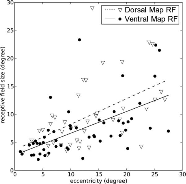
Receptive field sizes as a function of the eccentricity of their centers. Only non-vague (moderate and brisk) units in penetrations showing clear reversals of RF progression were included in the analysis. Straight lines are linear regressions for the two classes of units. The eccentricities were translated from distance on the tangent screen to the view angle from area centralis and the receptive field sizes were calculated as the square root of the area of the ellipses used to model the receptive fields. Receptive field sizes increase with eccentricity in both maps, and receptive fields in the dorsal map were slightly larger than receptive fields in the ventral map at comparable eccentricities.

Compared to the two maps of macaque monkey lateral pulvinar (Bender, 1981, Fig.10), the maps in bush baby pulvinar had neurons with larger receptive fields for the same eccentricity. These pulvinar cells also featured receptive field sizes comparable to cells in bush baby V2 (Allison & Casagrande, 1994), and larger receptive fields than found in bush baby V1 cells (DeBruyn et al., 1993). The same relationship was found in macaque monkey, where pulvinar cell receptive fields were larger in size than V1 cells (Bender, 1981; Hubel & Wiesel, 1974), suggesting that if V1 provides the visual drive to these maps there is convergence of input to pulvinar.

Area Medial to the Two Maps

A few penetrations suggested that more visual areas may exist medial to the two identified maps. In these medial penetrations, receptive fields were encountered that were in a drastically different location than would be predicted in a typical receptive field progression through the dorsal and ventral maps. Some of these receptive fields were encountered at the beginning of some penetrations, before we entered the dorsal map (see Figure 6E). The rest were encountered deep in penetrations below cells showing receptive field progressions typical for the ventral map (see Figure 7E). Among the cells encountered after the ventral map, some also displayed very large receptive fields, often encompassing the full contralateral visual field. Others showed receptive fields located well into the ipsilateral visual field, or extending over VM into the ipsilateral visual field. In each of the latter cases the location of the optic disks was checked to ensure that the eyes had not moved.

Discussion

In this study, we identified three architectonic subdivisions in bush baby PI. Two electrophysiologically defined retinotopic maps were found, one confined in PL and the other within ventral PL and PIcl, a new subdivision of PI. The central vision representations of both maps were found at the posterior end of the border between the two maps. We found that bush baby pulvinar receptive fields were slightly larger than those found in the macaque monkey, and they increased in size with eccentricity. We did not find qualitative differences in stimulus preferences between cells in the two maps. Below we discuss how the architectonic structure of bush baby PI and PL relate to their connection patterns and how their connections correlate with the retinotopic maps. We compare the retinotopic pulvinar maps in bush baby with those found in the New and Old World simian species, represented by macaque and cebus monkey, respectively. Finally, we propose two models of retinotopic organization that can account for bush baby pulvinar maps and the maps described previously in macaque monkey.

Architecture and Connections

With both architectonic and retinotopic information, we were able to establish subdivisions within bush baby PI that appear consistent with the subdivisions described in simian species (Stepniewska & Kaas, 1997; Gray et al., 1999). We used the nomenclature established in owl monkey since it appeared to fit best with the bush baby subdivisions (see Lin & Kaas, 1979). These subdivisions also bear similarity with PI subdivisions described in other simians. In owl monkey, PIm is defined uniquely by a dark myelin circle (Lin & Kaas, 1979). In macaque, CO staining of PI showed four bands demarcating PIcl, PIcm, PIm and PIp with alternating dark and light staining from lateral to medial (Gutierrez et al., 1995; Stepniewska & Kaas, 1997). In bush baby PIm showed a myelin circle, while PIcl, PIcm and PIm showed dark, light and dark alternating CO bands, suggesting homology with these subdivisions in simians.

A number of connectional studies in bush babies and macaques also support the chemoarchitectonic subdivisions we found in this study. In bush baby, both V1 and MT have been reported to employ two separate connections with PI areas that we defined as PIcl and PIm (Symonds & Kaas, 1978; Wall et al., 1982; Wong et al., 2009). Some connections with the temporal cortices have been found exclusively in PIcm among PI subdivisions (Raczkowski & Diamond, 1980; Raczkowski & Diamond, 1981). In macaque, PIcl and PIm also have been reported to have separate connections with MT (Ungerleider et al., 1984) and receive separate inputs from V1 (Gutierrez & Cusick, 1997). Also, several studies showed that V2 projects to PIcl (Kennedy & Bullier, 1985; Raczkowski & Diamond, 1980) but not PIm (O'Brien et al., 2002; Raczkowski & Diamond, 1980) in both bush baby and macaque. Some interspecies differences, however, have been reported to exist in the connection patterns between PI and higher visual areas. For example, the only PI subdivision that showed connections to DLr (the rostral area of the dorsolateral visual area, considered to overlap with V4 in macaque) was PIm in bush baby (Raczkowski & Diamond, 1981), and PIcm in macaque (Kaas & Lyon, 2007).

PL and PI have been reported to receive inputs from several subcortical visual areas, including the superficial layers of the superior colliculus (SC) and the parabigeminal nucleus (Diamond et al., 1992). Parabigeminal projections appeared to be located within PL and PIcl (Diamond et al., 1992). The superficial layers of the superior colliculus have been shown to project to the posterior half of PI, and to a thin dorsal layer in PL (Diamond et al., 1992). Baldwin et al. (2011) further reported two chemoarchitectonic subdivisions at the caudal end of PI that receive from SC. These areas were identified by immunostaining for the vesicular glutamate transporter 2 (vGluT2). We were unable to correlate these areas with the chemoarchitectonic subdivisions identified in this study. More subdivisions may be found in bush baby PI and PL but different chemoarchitectonic methods will be required.

Retinotopic Maps in Pulvinar and their connections with Visual Cortex

The map features we found electrophysiologically were consistent with those observed in connectional studies. As expected from the connectional patterns, we found that a localized point in the paracentral visual field was represented as a curved strip of cells in the pulvinar, running roughly anterior posterior. The two strips curve toward the border between the two maps at their anterior ends, and meet at some point. Anatomical examples that are similar to cross-sections of the eccentricity contours shown in Figure 4B can be seen in Symonds and Kaas (1978) showing V1 projections and Carey et al. (1979) showing retrograde labeling from V1. In the latter study when a series of injections were made in V1 from the central to the peripheral representation, the strips of labeled pulvinar cells moved both anteriorly and away from the border between the dorsal and ventral maps (Carey et al., 1979). This pattern is consistent with the representation of central vision at the medio-posterior end of the border between the two visuotopic maps. Consistent with our findings concerning the upper and lower visual field representations, the lateral part of PI/PL has been reported to connect to lateral V1, which represents the upper visual field (Raczkowski & Diamond, 1981), while medial part of PI/PL has been reported to connect to medial V1, which represents the lower visual field (Raczkowski & Diamond, 1981; Conley & Raczkowski, 1990; DeBruyn et al., 1993). The central-peripheral and upper-lower field axes in our maps are also consistent with those inferred from pulvinar-MT connections (see Wall et al., 1982; Wong et al., 2009).

The two pulvinar visuotopic maps have cortical connections only with the early visual cortices. Both maps have major connections with V1, V2, V3, and to a lesser extent MT (Raczkowski & Diamond, 1981). Reciprocal connections with the temporal visual areas were reported to be restricted to either PM or the medial and ventral border of PI (Raczkowski & Diamond, 1980; Raczkowski & Diamond, 1981). Connections with the posterior parietal cortex were only found in PM (Glendenning et al., 1975; Raczkowski & Diamond, 1981).

Prosimian and simian pulvinar

The pulvinar of simians, particularly the pulvinar of anthropoid primates, is generally larger than that of studied prosimians (Chalfin et al., 2007). In the Old World simian macaque, the pulvinar is rotated laterally and posteriorly in comparison to that of the bush baby. Once these transformations have been accounted for, most architectonic and visuotopic map features appear to correspond nicely between these two species. In bush baby, the dorsal and ventral maps are found lateral to PIm, while in macaque they are found ventral, lateral and posterior to the MT recipient zone of PIm, consistent with an overall pulvinar rotation. The lateral map in macaque is analogous to the dorsal bush baby map we report here, and the inferior macaque map appears to correspond nicely to the ventral bush baby map. The upper field is represented laterally in both bush baby maps, and ventrally in both macaque maps. Under the same transformation the vertical sheet of HM representation in bush baby lies at a similar position in pulvinar as the mostly horizontal sheet of HM representation in macaque. Two major differences, however, exist between the two species. In macaque pulvinar, VM is represented on the border between the two maps, while in bush baby pulvinar VM is represented the posterior and media edges of that border. Additionally, in macaque the lateral map has a second order representation of the visual field. In other words, the representation of the horizontal meridian is split on the lateral surface of PL: the upper and lower visual field representations are not joined at the horizontal meridian. First order representations are those where adjacent points of the same hemifield always map to adjacent points in the brain such as in the primary visual cortex or middle temporal cortex. In contrast second order representations are maps that contain a discontinuity in their representation in the brain and adjacent points are not necessarily represented in adjacent pieces of tissue as is the case for the second visual area (V2) in primates (Allman & Kaas, 1974) much like in V2, where the HM representation is split to form its anterior border. In bush baby, by contrast with macaque monkey, both pulvinar visuotopic maps appear to have first order representations.

The two maps in bush baby pulvinar are similar in visual field representation to the ventrolateral map in the New World cebus pulvinar. The ventrolateral cebus map reported in Gattass et al. (1978) may, in fact, consists of two individual retinotopic maps. Cebus pulvinar is rotated laterally and posteriorly compared to bush baby pulvinar, as in the macaque. Instead of being located at the medio-posterior pole as in bush baby pulvinar maps, the central vision representation of the ventrolateral pulvinar map is located on its latero-anterior border in cebus. If the bush baby pulvinar maps are rotated, most bush baby map features align nicely with those reported for the cebus ventrolateral map in pulvinar. These features include the shapes of both the VM and HM representations and their spatial relation (compare Figures 6A and 7A of this paper to Figures 4C and 5 in Gattass et al., 1978). Given its relation with the two bush baby pulvinar maps, the ventrolateral map in cebus pulvinar can be divided into two maps along the horizontal extension of the VM representation, where penetrations showed a reversal of receptive field progressions similar to the ones seen in bush baby. That border runs from the dorso-anterior end of the ventrolateral map to its ventro-posterior end. Since that border in cebus is not horizontal, however, double representations were not apparent in individual penetrations. Instead, anterior penetrations can be predicted to encounter cells in the ventral visuotopic map with receptive fields adjacent to those of belonging to posterior cells in the dorsal visuotopic map. Indeed, we can see examples of this double representation in the A+2 and A+0 penetrations in Figure 4 of Gattass et al. (1978), where the receptive fields in A+2 after the reversal matched the receptive fields in A+0 before the reversal. Additionally, the cebus dorso-medial map appeared to be located in the equivalent position to the dorsal medial PL (Pdm) in macaque (Petersen et al., 1985), which might correspond to a separate map dorso-anterior to the dorsal map in bush baby. The latter would require more data to confirm, however.

A partial pulvinar map representing the visual field beyond 5 degrees from central vision had been reported in the inferior pulvinar of the simian species owl monkey (Allman et al., 1972). Given that owl monkey visual pulvinar has been reported to be similar to bush baby visual pulvinar in both connection patterns (Graham et al., 1979) and architectonic features (Allman et al., 1972; Lin and Kaas, 1979), it is not surprising that the partial map reported in owl monkey PI showed many features in common with the ventral map we identified in bush baby, including the relative location of upper-lower field representation and central-peripheral representation (Allman et al., 1972). The major difference is that owl monkey PI was reported to be fully occupied by a single retinotopic map, instead of having a medial section not included in the major map. This feature is in contrast to later connectional findings that PIm in owl monkey had its own visual field representation separate from the map in PIc (Lin and Kaas, 1979, Graham et al., 1979). It was likely that the sparse sampling in this early electrophyisiology study was not enough to distinguish the two separate maps in PIcl and PIm.

The second order representation reported in the lateral map of macaque pulvinar appears not to be shared by either cebus or bush baby. Given the orientation of the maps in bush baby, for the dorsal map to have a second order representation most vertical penetrations should have started with receptive fields near HM, yet only a small part of our observed penetrations showed this feature. The cebus ventrolateral pulvinar map is reported as having straight, parallel iso-elevation contours (Gattass et al., 1978). Regardless of whether cebus ventrolateral pulvinar map consists of one or two maps this result suggests that there is no second order map in this area. The second order representation reported in macaque pulvinar map is thus specific to this species and suggests that this organization evolved separately in Old World simians.

A New Model for Maps in Thalamic Nuclei

The visual field is mapped onto the two dimensional sheet on the retina but is represented in a three dimensional volume in structures such as the pulvinar. Although the visual field is roughly represented the same way in different primates there are significant differences in detail. At least two models of visual field mapping exist in primate thalamus.

In the maps reported in macaque pulvinar the VM representation covers half the surface of the map. Both HM and VM are represented as curved sheets. The central vision is represented as a long curve on the intersection between HM and VM representations. Map features like the representations of VM, HM and the central vision are one dimension higher than the visual field features they represent: the central vision, a point, is represented as a curve, and VM, a line, is represented as a sheet. There exist perfect iso-projection curves for each of the two macaque pulvinar maps such that each point on the same curve represents the same location in the visual field (Bender, 1981). In other words, when sliced perpendicular to local iso-projection curves, each slab of the map contains the full representation of the contralateral visual field. The way the pulvinar maps represent the visual field as described in macaque is similar to that of V1 and LGN. In both of these areas, the visual field is mapped onto one surface, with a column made of cells from different layers representing the same point in the visual field. With this organization, different visual functions could potentially be carried out in different slabs of the same map. One such hypothesis concerning pulvinar states that more posterior slabs relay visual signals between V1 and V2, while more anterior slabs relay signal between gradually higher levels in the visual hierarchy (Shipp, 2003, Fig.5-6).

In contrast to the macaque pulvinar maps, the central vision is represented as single points in both bush baby pulvinar maps, and VM is represented as a curve in both maps. In each of the maps, the representation of the elevation axis is parallel to the VM representation, and the azimuth axis is represented on the polar axis of a polar coordinate system on planes perpendicular to the VM representation. This organization leaves the polar angle as the iso-projection axis. The iso-projection curves are roughly concentric to the central vision representation and parallel to the HM representation. Unlike the organization described in macaque pulvinar, there is no obvious way to subdivide such maps into divisions with full visual field representations. As a result, cells with different functions are more likely to be mixed in bush baby pulvinar rather than clustered. Indeed we found cells with different visual responses mixed in bush baby pulvinar.

The partial inferior map reported in owl monkey pulvinar was described as resembling the one model represented by macaque pulvinar maps, with its representation of central vision on a line at the middle of its dorsal surface. However, details of that map near its central vision representation are lacking so we do not know whether this is indeed the case. As discussed in the previous section, cebus pulvinar maps showed a focal representation of central vision which fits more with the map model for bush baby than with that of the macaque monkey but again the data for the latter study are sparse so it is still unclear how the pulvinar maps are organized in either owl monkey or cebus monkey.

These two different types of visuotopic map organization are diagrammed in figure 11. Panel A shows a model of the macaque pulvinar inferior map abstracted from the diagrams in Figure 11 of Bender (1981) , while in panel B the model shows how the visual field is mapped in the bush baby pulvinar. The difference in the shapes of certain map features, such as the central vision representation and VM, can be easily visualized. These models can be applied to other thalamic nuclei where 2-D sensory sheets are represented in a 3-D volume and where specific aspects of the sensory sheet are emphasized. For example, the map organization reflected in primate LGN conforms to the former model represented also by the macaque pulvinar. Cells with different functions achieve a higher level of clustering in the former model compared to the latter. This difference in pulvinar map organization may reflect the higher levels of differentiation in Old World simian pulvinar compared to both prosimian and New World simian pulvinar.

11.

Two ways that a 2-D contralateral visual field could be represented in a 3-D brain structure. A: retinotopy of the inferior map of the macaque pulvinar adapted from Figure 11 of Bender, 1981, and an simplified model of that map in the upper-right corner. B: retinotopy of the inferior map in bush baby pulvinar, and its simplified model in two different views. In the simplified models, stars indicate central vision representations. Purple lines show the intersection of the horizontal meridian (HM) representations with the structure surface for the simplified model, and HM for the coronal sections. The vertical meridian (VM) is shown either as a green surface or a green line. Note that most of the visible intersection between HM and the surface in the left panel is also the intersection between the HM and VM representations, and thus the central vision representation. Thin dotted lines are iso-eccentricity contours, with lower eccentricity represented by denser dotted lines. The VM representation line in B is only on the structure surface, in contrast to all other lines representing the intersection between a plane in the structure and the structure surface. Numerals indicate eccentricity in degrees.

LITERATURE CITED

- Allison JD, Casagrande VA. Receptive field structure of V2 neurons in the prosimian primate Galago crassicaudatus. Society for Neuroscience. 1994;20:1741. (Abs.) [Google Scholar]
- Allman JM, Kaas JH. The organization of the second visual area (V II) in the owl monkey: a second order transformation of the visual hemifield. Brain Res. 1974;76:247–265. doi: 10.1016/0006-8993(74)90458-2. [DOI] [PubMed] [Google Scholar]
- Allman JM, Kaas JH, Lane RH. The middle temporal visual area (MT) in the bushbaby, Galago senegalensis. Brain Res. 1973;57:197–202. doi: 10.1016/0006-8993(73)90576-3. [DOI] [PubMed] [Google Scholar]
- Allman JM, Kaas JH, Lane RH, Miezin FM. A representation of the visual field in the inferior nucleus of the pulvinar in the owl monkey. Brain Res. 1972;40:291–302. doi: 10.1016/0006-8993(72)90135-7. [DOI] [PubMed] [Google Scholar]
- Arend I, Rafal RD, Ward R. Spatial and temporal deficits are regionally dissociable in patients with pulvinar lesions. Brain. 2008;131:2140–2152. doi: 10.1093/brain/awn135. [DOI] [PubMed] [Google Scholar]
- Baldwin MKL, Balaram P, Kaas JH. Superior colliculus connections and VGLUT2 expression within visual thalamus of prosimian galagos (Otolemur garnetti).. Program No. 817.17. 2011 Neuroscience Meeting Planner; Washington, DC: Society for Neuroscience. 2011. 2011. Online. [Google Scholar]
- Bender DB. Retinotopic organization of macaque pulvinar. J Neurophysiol. 1981;46:672–693. doi: 10.1152/jn.1981.46.3.672. [DOI] [PubMed] [Google Scholar]
- Bender DB. Receptive-field properties of neurons in the macaque inferior pulvinar. J Neurophysiol. 1982;48:1–17. doi: 10.1152/jn.1982.48.1.1. [DOI] [PubMed] [Google Scholar]
- Berman RA, Wurtz RH. Signals conveyed in the pulvinar pathway from superior colliculus to cortical area MT. J Neurosci. 2011;31:373–384. doi: 10.1523/JNEUROSCI.4738-10.2011. [DOI] [PMC free article] [PubMed] [Google Scholar]
- Boyd JD, Matsubara JA. Laminar and columnar patterns of geniculocortical projections in the cat: relationship to cytochrome oxidase. J Comp Neurol. 1996;365:659–682. doi: 10.1002/(SICI)1096-9861(19960219)365:4<659::AID-CNE11>3.0.CO;2-C. [DOI] [PubMed] [Google Scholar]
- Carey RG, Fitzpatrick D, Diamond IT. Layer I of striate cortex of Tupaia glis and Galago senegalensis: Projections from thalamus and claustrum revealed by retrograde transport of horseradish peroxidase. J Comp Neurol. 1979;186:393–437. doi: 10.1002/cne.901860306. [DOI] [PubMed] [Google Scholar]
- Chalfin BP, Cheung DT, Muniz JAPC, de Lima Silveira LC, Finlay BL. Scaling of neuron number and volume of the pulvinar complex in New World primates: comparisons with humans, other primates, and mammals. J Comp Neurol. 2007;504:265–274. doi: 10.1002/cne.21406. [DOI] [PubMed] [Google Scholar]
- Conley M, Raczkowski D. Sublaminar organization within layer VI of the striate cortex in Galago. J Comp Neurol. 1990;302:425–436. doi: 10.1002/cne.903020218. [DOI] [PubMed] [Google Scholar]
- DeBruyn E, Casagrande VA, Beck PD, Bonds AB. Visual resolution and sensitivity of single cells in the primary visual cortex (V1) of a nocturnal primate (bush baby): correlations with cortical layers and cytochrome oxidase patterns. J Neurophysiol. 1993;69:3–18. doi: 10.1152/jn.1993.69.1.3. [DOI] [PubMed] [Google Scholar]
- del Río MR, DeFelipe J. A light and electron microscopic study of calbindin D-28k immunoreactive double bouquet cells in the human temporal cortex. Brain Res. 1995;690:133–140. doi: 10.1016/0006-8993(95)00641-3. [DOI] [PubMed] [Google Scholar]
- Diamond IT, Fitzpatrick D, Conley M. A projection from the parabigeminal nucleus to the pulvinar nucleus in Galago. J Comp Neurol. 1992;316:375–382. doi: 10.1002/cne.903160308. [DOI] [PubMed] [Google Scholar]
- Emmers R, Akert K, Woolsey CN, editors. A stereotaxic atlas of the brain of the squirrel monkey (Saimiri sciureus). 1st ed. University of Wisconsin Press Madison; 1963. [Google Scholar]
- Van Essen DC. Corticocortical and thalamocortical information flow in the primate visual system. Prog Brain Res. 2005;149:173–185. doi: 10.1016/S0079-6123(05)49013-5. [DOI] [PubMed] [Google Scholar]
- Gallyas F. Silver staining of myelin by means of physical development. Neurol Res. 1979;1:203–209. doi: 10.1080/01616412.1979.11739553. [DOI] [PubMed] [Google Scholar]
- Gattass R, Oswaldo-Cruz E, Sousa APB. Visuotopic organization of the cebus pulvinar: a double representation of the contralateral hemifield. Brain Res. 1978;152:1–16. doi: 10.1016/0006-8993(78)90130-0. [DOI] [PubMed] [Google Scholar]
- Geneser-Jensen FA, Blackstad TW. Distribution of acetyl cholinesterase in the hippocampal region of the guinea pig. Cell Tissue Res. 1971;114:460–481. doi: 10.1007/BF00325634. [DOI] [PubMed] [Google Scholar]
- Glendenning K, Hall J, Diamond IT, Hall W. The pulvinar nucleus of Galago senegalensis. J Comp Neurol. 1975;161:419–457. doi: 10.1002/cne.901610309. [DOI] [PubMed] [Google Scholar]
- Gray DN, Gutierrez C, Cusick CG. Neurochemical organization of inferior pulvinar complex in squirrel monkeys and macaques revealed by acetylcholinesterase histochemistry, calbindin and Cat-301 immunostaining, and Wisteria floribunda agglutinin binding. J Comp Neurol. 1999;409:452–468. doi: 10.1002/(sici)1096-9861(19990705)409:3<452::aid-cne9>3.0.co;2-i. [DOI] [PubMed] [Google Scholar]
- Gutierrez C, Cusick CG. Area V1 in macaque monkeys projects to multiple histochemically defined subdivisions of the inferior pulvinar complex. Brain Res. 1997;765:349–356. doi: 10.1016/s0006-8993(97)00696-3. [DOI] [PubMed] [Google Scholar]
- Gutierrez C, Yaun A, Cusick CG. Neurochemical subdivisions of the inferior pulvinar in macaque monkeys. J Comp Neurol. 1995;363:545–562. doi: 10.1002/cne.903630404. [DOI] [PubMed] [Google Scholar]
- Hendry SHC, Reid RC. The koniocellular pathway in primate vision. Annu Rev Neurosci. 2000;23:127–153. doi: 10.1146/annurev.neuro.23.1.127. [DOI] [PubMed] [Google Scholar]
- Hubel DH, Wiesel TN. Uniformity of monkey striate cortex: a parallel relationship between field size, scatter, and magnification factor. J Comp Neurol. 1974;158:295–305. doi: 10.1002/cne.901580305. [DOI] [PubMed] [Google Scholar]
- Huerta MF, Krubitzer LA, Kaas JH. Frontal eye field as defined by intracortical microstimulation in squirrel monkeys, owl monkeys, and macaque monkeys: I. Subcortical connections. J Comp Neurol. 1986;253:415–439. doi: 10.1002/cne.902530402. [DOI] [PubMed] [Google Scholar]
- Jerison HJ. Brain, body and encephalization in early primates. J Hum Evol. 1979;8:615–635. [Google Scholar]
- Johnson J, Casagrande VA. Distribution of calcium-binding proteins within the parallel visual pathways of a primate (Galago crassicaudatus). J Comp Neurol. 1995;356:238–260. doi: 10.1002/cne.903560208. [DOI] [PubMed] [Google Scholar]
- Kaas JH, Lyon DC. Pulvinar contributions to the dorsal and ventral streams of visual processing in primates. Brain Res Rev. 2007;55:285–296. doi: 10.1016/j.brainresrev.2007.02.008. [DOI] [PMC free article] [PubMed] [Google Scholar]
- Kennedy H, Bullier J. A double-labeling investigation of the afferent connectivity to cortical areas V1 and V2 of the macaque monkey. J Neurosci. 1985;5:2815–2830. doi: 10.1523/JNEUROSCI.05-10-02815.1985. [DOI] [PMC free article] [PubMed] [Google Scholar]
- Lin CS, Kaas JH. The inferior pulvinar complex in owl monkeys: architectonic subdivisions and patterns of input from the superior colliculus and subdivisions of visual cortex. J Comp Neurol. 1979;187:655–678. doi: 10.1002/cne.901870403. [DOI] [PubMed] [Google Scholar]
- Lysakowski A, Standage GP, Benevento LA. Histochemical and architectonic differentiation of zones of pretectal and collicular inputs to the pulvinar and dorsal lateral geniculate nuclei in the macaque. J Comp Neurol. 1986;250:431–448. doi: 10.1002/cne.902500403. [DOI] [PubMed] [Google Scholar]
- Merabet LU, Desautels A, Minville K, Casanova C. Motion integration in a thalamic visual nucleus. Nature. 1998;396:265–268. doi: 10.1038/24382. [DOI] [PubMed] [Google Scholar]
- O'Brien BJ, Abel PL, Olavarria JF. Connections of calbindin-D28k-defined subdivisions in inferior pulvinar with visual areas V2, V4 and MT in macaque monkeys. Thalamus & Related Systems. 2002;1:317–330. [Google Scholar]
- Petersen SE, Robinson DL, Keys W. Pulvinar nuclei of the behaving rhesus monkey: visual responses and their modulation. J Neurophysiol. 1985;54:867–886. doi: 10.1152/jn.1985.54.4.867. [DOI] [PubMed] [Google Scholar]
- Petersen SE, Robinson DL, Morris JD. Contributions of the pulvinar to visual spatial attention. Neuropsychologia. 1987;25:97–105. doi: 10.1016/0028-3932(87)90046-7. [DOI] [PubMed] [Google Scholar]
- Raczkowski D, Diamond IT. Cortical connections of the pulvinar nucleus in Galago. J Comp Neurol. 1980;193:1–40. doi: 10.1002/cne.901930102. [DOI] [PubMed] [Google Scholar]
- Raczkowski D, Diamond IT. Projections from the superior colliculus and the neocortex to the pulvinar nucleus in Galago. J Comp Neurol. 1981;200:231–254. doi: 10.1002/cne.902000205. [DOI] [PubMed] [Google Scholar]
- Robinson DL, Petersen SE. Responses of pulvinar neurons to real and self-induced stimulus movement. Brain Res. 1985;338:392–394. doi: 10.1016/0006-8993(85)90176-3. [DOI] [PubMed] [Google Scholar]
- Sherman SM. The thalamus is more than just a relay. Curr Opin Neurobiol. 2007;17:417–422. doi: 10.1016/j.conb.2007.07.003. [DOI] [PMC free article] [PubMed] [Google Scholar]
- Shipp S. The functional logic of cortico-pulvinar connections. Philos Trans R Soc Lond B Biol Sci. 2003;358:1605–1624. doi: 10.1098/rstb.2002.1213. [DOI] [PMC free article] [PubMed] [Google Scholar]
- Stepniewska I, Kaas JH. Architectonic subdivisions of the inferior pulvinar in New World and Old World monkeys. Vis Neurosci. 1997;14:1043–1060. doi: 10.1017/s0952523800011767. [DOI] [PubMed] [Google Scholar]
- Symonds LL, Kaas JH. Connections of striate cortex in the prosimian, Galago senegalensis. J Comp Neurol. 1978;181:477–511. doi: 10.1002/cne.901810304. [DOI] [PubMed] [Google Scholar]
- Theyel B, Llano D, Sherman SM. The corticothalamocortical circuit drives higher-order cortex in the mouse. Nat Neurosci. 2010;13:84–88. doi: 10.1038/nn.2449. [DOI] [PMC free article] [PubMed] [Google Scholar]
- Ungerleider LG, Desimone R, Galkin TW, Mishkin M. Subcortical projections of area MT in the macaque. J Comp Neurol. 1984;223:368–386. doi: 10.1002/cne.902230304. [DOI] [PubMed] [Google Scholar]
- Walker AE, editor. The Primate Thalamus. University of Chicago press; 1938. [Google Scholar]
- Wall JT, Symonds LL, Kaas JH. Cortical and subcortical projections of the middle temporal area (MT) and adjacent cortex in galagos. J Comp Neurol. 1982;211:193–214. doi: 10.1002/cne.902110208. [DOI] [PubMed] [Google Scholar]
- Wong P, Collins CE, Baldwin MKL, Kaas JH. Cortical connections of the visual pulvinar complex in prosimian galagos (Otolemur garnettii). J Comp Neurol. 2009;517:493–511. doi: 10.1002/cne.22162. [DOI] [PMC free article] [PubMed] [Google Scholar]
- Wong-Riley M. Changes in the visual system of monocularly sutured or enucleated cats demonstrable with cytochrome oxidase histochemistry. Brain Res. 1979;171:11–28. doi: 10.1016/0006-8993(79)90728-5. [DOI] [PubMed] [Google Scholar]