Adaptive Image Segmentation for Robust Measurement of Longitudinal Brain Tissue Change

Abstract

We present a method that significantly improves magnetic resonance imaging (MRI) based brain tissue segmentation by modeling the topography of boundaries between tissue compartments. Edge operators are used to identify tissue interfaces and thereby more realistically model tissue label dependencies between adjacent voxels on opposite sides of an interface. When applied to a synthetic MRI template corrupted by additive noise, it provided more consistent tissue labeling across noise levels than two commonly used methods (FAST and SPM5). When applied to longitudinal MRI series it provided lesser variability in individual trajectories of tissue change, suggesting superior ability to discriminate real tissue change from noise. These results suggest that this method may be useful for robust longitudinal brain tissue change estimation.

I. Introduction

Brain imaging studies increasingly depend on the ability to accurately and consistently identify changes in tissue volumes over time from serial MRI. Many methods for assigning tissue labels to pixels in an individual MRI are applicable to this problem: such methods are applied separately to each individual MRI in a longitudinal series. Typically these approaches use automatic initialization (see e.g. [1, 2]) together with the expectation-maximization (EM) algorithm [3] and Markov random fields (MRF) (see e.g. [4, 5]) to estimate Bayesian maximum a posteriori (MAP) tissue labels [4, 6] that agree with prior knowledge of tissue appearance and are situated in a plausible spatial arrangement.

Comparatively little attention, however, has been paid to the problem of tissue segmentation consistency over time. In many cases, volumes of specific tissue compartments are expected to increase (e.g., gray matter in typically-developing children) or decrease (e.g. gray matter in elders with Alzheimer’s disease) steadily over time in any individual; methods that separately segment each image in a longitudinal series are not strictly required to enforce such plausibility. SIENA [7, 8] is one method that does attempt to enforce plausible longitudinal change, but it is aimed at reporting overall brain tissue loss rather than changes to specific compartments (i.e., gray matter, white matter, and cerebrospinal fluid – CSF). In addition its performance has been shown to deteriorate in the presence of noise or MRI field non-uniformities [9]. Another approach uses a true “4-D” image framework to ensure that tissue classification of an image voxel is consistent with its neighbor locations in both space and time [10]. This is accomplished using warps to register images from all time points to a template, followed by segmentation that encourages both spatial and temporal consistency in labels. State-of-the-art MAP algorithms for tissue appearance and spatial arrangement do not scale well to segmentation problems involving many images in a series; thus, approaches of this type are forced to make approximations that amount to playing a tradeoff between temporal consistency and accuracy of segmentation at any given time point.

In this paper we propose that incorporating robust tissue boundary estimates into tissue segmentation of individual images in a longitudinal series can lead to greater plausibility in tissue change estimates. In an MRF model of tissue spatial arrangement, we use tissue boundaries estimated from edge operators to encourage differing tissue labels on opposite sides of a boundary. We compare this Gradient-based Segmentation (GSeg) method against two readily available and commonly used tools, SPM5 (http://www.fil.ion.ucl.ac.uk/spm/) [11] and FAST (http://www.fmrib.ox.ac.uk/fsl/) [5], for segmentation performance on an individual synthetic image corrupted by varying degrees of noise, and on real longitudinal MRI series of elderly individuals. We hypothesized that incorporating boundary information into an MRF would enable greater robustness against noise and improved longitudinal consistency of tissue change estimates.

II. Methods

A. Maximum a Posteriori (MAP) Algorithm

The image is defined as an array y of intensities, with one entry y_i for each pixel i. A segmentation of the image is a corresponding array of labels x, such that each pixel label is drawn from a small set of K possible labels {L₁, L₂, …, L_K}.

Here K will be 3 or 4, corresponding to CSF, gray matter, normal white matter, and optionally white matter hyperintensities. Given a conditional probability density p for the segmentation labels conditioned on the image intensities y, we seek an optimal labeling, x*, such that

$$\mathit{x}\ast =arg{max}_{\mathit{x}}p(\mathit{x}\mid \mathit{y}).$$ (1)

Using Bayes’ Theorem, this is equivalent to solving

$${\mathit{x}}^{\ast }=arg{max}_{\mathit{x}}p(\mathit{y}\mid \mathit{x})p(\mathit{x}).$$ (2)

The two components in equation (2) are the measurement model p(y | x) and the prior model p(x). The measurement model requires that the intensity of every pixel assigned to a particular tissue class be drawn from a Gaussian distribution whose mean and standard deviation are estimated at the time of segmentation. The prior model assumes that x is a Markov random field (MRF) so that the prior probability of a tissue label x_i at voxel i depends only on the labels of neighboring voxels. The prior model quantifies the degree to which x_i and neighbors have a plausible assignment of labels, based on the number of neighbors whose labels agree with x_i as well as an expected frequency of each possible label. It is expressed as a Gibbs distribution [4] of the form

$$p(x_i)=\frac{1}{Z}exp\left(-V_c(x_i)-{\alpha }_k\delta (x_i=k)\right),$$ (3)

where Z is a normalizing constant, δ is an indicator returning 1 if the condition inside the parentheses is true and zero otherwise, and α_k measures the weight of belonging to tissue class k. The V_c have the format

$$V_c(x_i)={\beta }_1{f}_1(x_i)+{\beta }_2{f}_2(x_i)$$ (4)

where f₁ and f₂ are functions depending on the tissue class labels of first-order and second-order neighbors, respectively, and the β coefficients are determined at each iteration [4]. We select the form of f₁ and f₂ to adapt the prior to the presence of edges, as described below.

We use an iterative EM optimization to interleave estimation of x* based on current α and β estimates and Gaussian intensity distribution parameters, with estimation of α, β, and Gaussian parameters based on the current x*[4].

B. Adaptive Prior Model

Our prior model weights label differences between x_i and its neighbors differently depending on the likelihood that a tissue interface passes near location i, as determined by the image intensity gradient magnitude. Far from tissue boundaries, we encourage homogeneous tissue neighborhoods (i.e. encourage all x_j to be equal) by selecting f₁ and f₂ functions that take minimal values when this is true. Conversely, near edges different f₁ and f₂ functions are chosen that are minimized when the neighborhoods consist of two equally represented classes.

In particular, far from edges both f₂ and f₂ take on this

$$f(x_i==L_j)=\frac{N}{2}-n(L_j)$$ (5)

for tissue class L_j, where n(L_j) is the number of neighbors of voxel i that are labeled L_j, and N is the total number of neighbors. It is minimal (negative) when all neighbors are of the same class L _j as voxel i. Near edges, by contrast,

$$f(x_i==L_j)=\left|\frac{N}{2}-n(L_j)\right|+\prod _{k\ne j}n(L_k)$$ (6)

The first term of this function is minimized (zero) when exactly half of the pixels in the neighborhood are labeled L_j. The second term is minimized when the product is zero, i.e. n(L_k) = ₀ for some tissue class L _k ≠ L _j. Thus we reward an edge voxel x_i where half the neighbor voxels are of the same class as x_i, with the rest being all of one other class. Given the format selection of the f functions to use at voxel i, we label x_i as the class L_j for which V_c(x_i) is minimized.

To select the format of the f functions at each voxel, we calculate the image gradient magnitude by convolving the image with derivative of Gaussian filters in the x, y and z directions (2.4 mm FWHM), calculating the Euclidean (sum of squares) gradient magnitude from the partial derivatives. We construct the histogram of gradient magnitude values and set a threshold for edge proximity to be the gradient magnitude where the maximum histogram peak occurs (i.e. the histogram “mode” or most frequent value of the gradient magnitude). Voxels whose gradient magnitudes are above this threshold are considered to be near edges and assigned the set of f functions (6); other voxels use the functions (5).

C. Automatic Initialization using Template-Based Tissue Masks

Our EM procedure alternates between estimating voxel labels and estimating MRF parameters. We initialize the labels using template-based tissue probability maps generated in-house.Each tissue probability map is warped onto the native subject image via a high-dimensional B-spline warping [12] previously computed to match a normal elderly minimal deformation template [13] with the subject brain. When the warped probability masks are overlaid on the native brain image, an initial classification x is made labeling each voxel with the tissue class corresponding to the highest value among the three warped probability masks.

III. Results

We compare the performance of our method against FAST and SPM5 using visual comparisons and a segmentation of the BrainWeb template. We then analyze the utility of the segmentations for measuring longitudinal tissue change. Finally, we illustrate the contributions of the adaptive prior to segmentation accuracy.

A. Comparisons Using the Synthetic Image Template

Each of the three methods were used to segment the BrainWeb [14] (http://www.bic.mni.mcgill.ca/brainweb/) template image at two levels of random Gaussian noise: 3% and 5%.

Visual comparison of the BrainWeb segmentations is presented in Fig. 1. Segmented tissue boundaries appear comparable at low noise levels (3%–5%) across all methods with the exception of brainstem segmentation for FAST (black arrow in row 2): at 5% it appears (erroneously) white. The GSeg method did a better job of representing small sulci and finger-like extensions of the white matter into gray, though possibly overstating sulcal CSF.

Figure 1.

Segmentation of BrainWeb template at noise levels 3% (top row), 5% (bottom).

B. Statistical Analysis of Longitudinal Segmentation

We applied the three methods to brain MRI of 57 cognitively normal and 60 demented individuals from the ADNI study and compared one-year changes in gray matter, white matter, and CSF across methods [15]. Images from each individual’s baseline, 6 month, and 1 year visits were segmented by each method. Fig. 2 shows baseline and one-year results for a single subject. Methods were compared for within-person variation in tissue volumes over time. To assess within-person variation, for each segmentation method and tissue type a subject-specific linear regression was fit to the tissue volumes as a function of time, and the sum of squared residuals was recorded. Segmentations with lesser residuals may be able to quantify the true rate of change more precisely under an assumption of linear change, and thus may have greater utility for detecting true tissue change in longitudinal studies of brain aging.

Figure 2.

Comparison of segmentations of a single subject at baseline (top row) and one year scan (bottom).

We compared methods using a randomized block analysis of variance (ANOVA), with subjects as blocks, methods as fixed effects, and the logarithm of the sum of squared residuals as the outcome measure. Post-hoc pair wise comparisons between the methods were performed, with adjustments to the p-values using the Tukey Honestly Significant Differences (HSD) approach to account for multiple comparisons. Freidman’s rank test and the corresponding rank-based multiple comparison adjustment were used if the assumptions of the ANOVA were not met by the data. Analyses were conducted separately for AD and Normal subjects and p<0.05 was considered statistically significant. For longitudinal gray matter change in AD subjects there was a significant difference between methods in within-person variation (Fig. 3 top, p<0.01), with GSeg showing significantly less within-person variation than both FAST and SPM (p<0.05, adjusted) and FAST having intermediate variability between GSeg and SPM. In Normal subjects there was a significant difference between methods in within-person variability (Fig. 3 bottom, p<0.05). SPM had significantly greater variability than GSeg (p<0.05 adjusted), but GSeg and FAST were not significantly different.

Figure 3.

Plots of one-year trajectories of gray matter volume for the AD and normal groups. The average trajectory for each method is shown in black. Top row: AD group. Bottom: Normal.

C. Contribution of Adaptive Prior

Fig. 4 shows samples of segmentation of the BrainWeb template with 3% noise, using the adaptive prior (equations (5–6)) compared with a prior that favors homogeneous tissue neighborhoods everywhere [4]. Clear differences between the panels are visible. The boundary between lentiform nucleus and cortical gray is more clearly delineated in the right panel. The middle panel merges the two gray areas whereas the adaptive technique keeps them separated. Similarly, sulci in the vicinity of the insula show greater coherence in the right panel.

Figure 4.

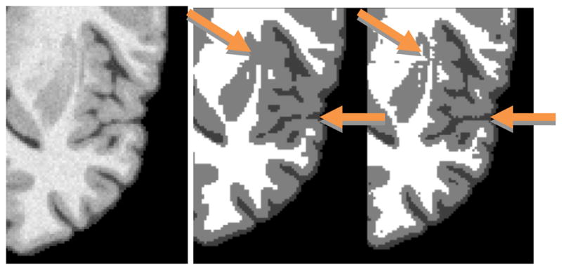
Segmentation of frontal cortex and subcortical nuclei without adaptive cliques (middle) and with (right). Compare quality of detail with template brain image (left).

IV. Discussion

Fig. 3 suggests that the GSeg method has achieved, on average, straight-line estimates of one-year longitudinal tissue change, unlike the other methods; this linear change may be more biologically plausible than nonlinear change, and therefore the GSeg method may be superior for quantifying longitudinal change. Examination of the single subject in Fig. 2 suggests that subcortical segmentation is a specific reason for its superiority. GSeg has a more robust and consistent representation of subcortical areas (thalamus and putamen) over time than either FAST or SPM5. Cortical details are also better represented in both GSeg and FAST than in SPM5. Fig. 4 suggests that the adaptive prior may be responsible for this performance advantage.

Our method does not simultaneously perform segmentation on a series of same-subject longitudinal scans. As discussed in the introduction, such true “4-D” techniques have tradeoffs of consistency over time vs. accuracy at single time points. Insead, our results have suggested that the adaptive edge-based technique, applied at single time points, results in improved segmentation detail which in turn gives improved consistency over images in a longitudinal series (Fig. 3).

The method has some limitations. Without further processing the segmented image tends to be noisier due to false positives in edge detection. This requires a final “speckle removal” step in the segmentation algorithm. Another potential imitation is that incorrect warping during the automatic label initialization could cause misclassification which may not be corrected during the EM phase, leading to tissue segmentation errors. We have found that this has not been a significant issue in most images.

V. Conclusion

We have compared three methods of image segmentation for consistency of tissue labels over varying levels of noise on the BrainWeb template and also for consistency over three-time-point longitudinal scans of AD and Normal subjects in the ADNI database. Our proposed method uses automatic initialization and an adaptive prior to achieve more robust segmentation in the presence of noise, particularly at tissue boundaries. Our results have indicated that these components can improve the segmentation of longitudinal image series compared to FAST and SPM.

References

- 1.Van Leemput K, et al. Automated Model-Based Tissue Classification of MR Images of the Brain. IEEE Transactions on Medical Imaging. 1999 Oct;18:897–908. doi: 10.1109/42.811270. [DOI] [PubMed] [Google Scholar]
- 2.Bazin PL, Pham DL. Homeomorphic brain image segmentation with topological and statistical atlases. Medical Image Analysis. 2008;12:616–625. doi: 10.1016/j.media.2008.06.008. [DOI] [PMC free article] [PubMed] [Google Scholar]
- 3.Dempster AP, et al. Maximum Likelihood from Incomplete Data via the EM Algorithm. Journal of the Royal Statistical Society Series B (Methodological) 1977;39:1–38. [Google Scholar]
- 4.Rajapakse JC, et al. Statistical Approach to Segmentation of Single-Channel Cerebral MR Images. IEEE Transactions on Medical Imaging. 1997 Apr;16:176–186. doi: 10.1109/42.563663. [DOI] [PubMed] [Google Scholar]
- 5.Zhang Y, et al. Segmentation of Brain MR Images Through Hidden Markov Random Field Model and Expectation-Maximization Algorithm. IEEE Transactions on Medical Imaging. 2001;20:45–57. doi: 10.1109/42.906424. [DOI] [PubMed] [Google Scholar]
- 6.Pohl KM, et al. A Bayesian model for joint segmentation and registration. NeuroImage. 2006;31:228–239. doi: 10.1016/j.neuroimage.2005.11.044. [DOI] [PubMed] [Google Scholar]
- 7.Smith SM, et al. Normalized Accurate Measurement of Longitudinal Brain Change. Journal of Computer Assisted Tomography. 2001;25:466–475. doi: 10.1097/00004728-200105000-00022. [DOI] [PubMed] [Google Scholar]
- 8.Smith SM, et al. Accurate, Robust, and Automated Longitudinal and Cross-Sectional Brain Change Analysis. NeuroImage. 2002;17:479–489. doi: 10.1006/nimg.2002.1040. [DOI] [PubMed] [Google Scholar]
- 9.Sharma S, et al. Use of simulated atrophy for performance analysis of brain atrophy estimation approaches. MICCAI 2009. 2009:566–574. doi: 10.1007/978-3-642-04271-3_69. [DOI] [PubMed] [Google Scholar]
- 10.Xue Z, et al. CLASSIC: Consistent Longitudinal Alignment and Segmentation for Serial Image Computing. NeuroImage. 2006;30:388–399. doi: 10.1016/j.neuroimage.2005.09.054. [DOI] [PubMed] [Google Scholar]
- 11.Ashburner J. A fast diffeomorphic image registration algorithm. NeuroImage. 2007;38:95–113. doi: 10.1016/j.neuroimage.2007.07.007. [DOI] [PubMed] [Google Scholar]
- 12.Kochunov P, et al. Regional Spatial Normalization: Toward and Optimal Target. Journal of Computer Assisted Tomography. 2001;25:805–816. doi: 10.1097/00004728-200109000-00023. [DOI] [PubMed] [Google Scholar]
- 13.Rueckert D, et al. Nonrigid registration using free-form deformations: applications to breast MR images. IEEE Transactions on Medical Imaging. 1999;18:712–720. doi: 10.1109/42.796284. [DOI] [PubMed] [Google Scholar]
- 14.Collins DL, et al. Design and Construction of a Realistic Digital Brain Phantom. IEEE Transactions on Medical Imaging. 1998 Jun;17:463–468. doi: 10.1109/42.712135. [DOI] [PubMed] [Google Scholar]
- 15.Meuller SG, et al. Ways toward an early diagnosis of Alzheimer’s disease: The Alzheimer’s Disease Neuroimaging Initiative (ADNI) Alzheimer’s and Dementia. 2005;1:55–66. doi: 10.1016/j.jalz.2005.06.003. [DOI] [PMC free article] [PubMed] [Google Scholar]