

Abstract
Reflectance measurement of breast tissue is influenced by the underlying chest wall, which is often tilted as seen by the detection probe. We develop an analytical solution of light propagation in a two-layer tissue structure with tilted interface and refractive index difference between the layers. We validate the analytical solution with Monte Carlo simulations and phantom experiments, and a good agreement is seen. The influence of varying the tilting angle of the interface on the reflectance is discussed for two types of layered structures. Further, we apply the developed analytical solution to obtain the optical properties of breast tissue and chest wall from clinical data. Inverse calculation using the developed solution applied to the data obtained from Monte Carlo simulations shows that the optical properties of both layers are obtained with higher accuracy as compared to using a simple two-layer model ignoring the interface tilt. This is expected to improve the accuracy in estimating the optical properties of breast tissue, thus enhancing the accuracy of optical tomography of breast tumors.
1. Introduction
Accurate evaluation of optical properties of embedded lesions from surface reflectance measurements is important and challenging in optical tomography.1–4 The biological tissues often contain layered structures, which contribute to the total reflectance measurements. A two-layer light propagation model is a simple and sufficiently accurate approximation to the imaging medium in most of the biomedical applications. Various numerical and analytical methods have been developed to study the time domain and frequency domain reflectance from layered tissue structures.5–12 Most of these methods were intended to analyze cases where the upper skin layer was relatively thinner (of the order of a few millimeters) such as skin above the subcutaneous fat layer or skin overlying the skull. In such applications the reflectance measured on the surface would be mostly influenced by the properties of the thicker second layer, which could then be easily retrieved. Several practical applications require imaging of two-layer structures where the upper layer is in general thicker (1–2 cm) and the interface between the layers may be tilted. Light-reflectance measurement from breast tissue is an example where the breast tissue and chest wall may have a titled interface with respect to the imaging probe. In such cases the reflectance measured at the upper tissue surface might have equal contributions from both layers or dominant contributions from either one of the layers, depending entirely on the layer thickness or tilt of the interface and the optical properties of the layers. Unlike in the case of imaging biological tissue under-neath thin skin, any simple approximation here would lead to large errors in analysis. Clinical results have shown that for patients whose breast tissue thickness is less than 1.5 to 2 cm, depending on average optical properties, the frequency domain reflectance measurement of both amplitude and phase acquired at a larger distance from a source often deviate from expected linear curves due to the presence of the chest wall.13,14 This is common for patients with smaller breasts when measurements are made in the supine position. A systematic analysis of the effects of the different layer properties and the titled interface on the reflectance measured at the tissue surface is necessary for developing any new image reconstruction techniques to account for the chest-wall-induced distortion effect.
Analytical solutions are preferred over numerical methods such as Monte Carlo calculations, which require intensive computation. Analytical solutions developed for frequency domain reflectance in two-layer tissue structure usually assume an average refractive index (RI) for both layers. It has already been shown that the estimated values of absorption and reduced scattering coefficients could be erroneous if the RI mismatch between layers were not considered.15 The RI mismatch changes the balance of energy inside the medium determining a temporal and spatial redistribution of light energy. The effect of RI mismatch for two-layer structures with a thinner upper layer has been investigated using the finite element method by Deghani et al.16 To the best of our knowledge, a simple analytical solution for a two-layer tissue structure with a thicker upper layer considering both RI mismatch and tilt of the interface does not exist in the literature. In this paper, we introduce such an analytical solution, which derives the basic methodology from the two-layer analytical solution developed by Dayan et al.6 and Kienle et al.5 However, the boundary conditions have been modified to incorporate the RI mismatch and the tilt at the interface of the layered structure, and the solutions are derived accordingly. To the best of our knowledge, there has been no prior work on the analysis of multilayer structures with a tilted interface. This is done as part of our efforts to understand and improve the clinical imaging of breast tissue where the reflectance measured at the surface is influenced by the chest-wall layer properties and the chest-wall layer may not be parallel to the imaging probe.13,14
The application of a two-layer model is mainly in estimating the average optical properties of tissue layers with improved accuracy compared to the semi-infinite approximation. The accurate optical properties would in turn enhance the quantification of functional imaging of tumors buried in such a medium. While this has been shown by several authors previously,5,7–11 all of them used signals detected at smaller source-detector separations that were sufficient for two-layer models with extremely thin upper layers. The property estimation of the second layer was more important for these studies since the tumors would be lying in the lower layer. For breast imaging where the upper layer (breast tissue) is typically between 1 and 4 cm, the signals detected at source-detector separations larger than 2 cm are of more relevance and hence any tilt at the interface between the breast tissue and the underlying chest wall is also of relevance for breast imaging as compared to the studies on layered structures with thinner upper layers of the order of a few millimeters.
This paper is organized as follows. In Section 2 we show the analytical derivation for light propagation in a two-layer tissue structure with a tilted interface. In Section 3 we discuss computational and numerical methods and experimental methods used to validate our newly developed solution. Results are presented in Section 4, and a summary is given in Section 5.
2. Theory
In this section, we present the derivation of an analytical solution for light propagation in a two-layer tissue structure, which could have an arbitrary tilt at the interface and refractive index mismatch between the layers.
Diffusion equations are solved for a two-layer turbid medium considering the most general case of an arbitrary tilted interface and also considering the refractive index difference between the two layers. The layer structure is shown in Fig. 1. An infinitely thin beam of frequency-modulated light is assumed to be incident perpendicularly on the top surface of a two-layer turbid medium, which would be diffused isotropically in the top layer at a depth of z = z0. The diffusion equation for the fluence rates (mm−2 s−1) is given as
Fig. 1.
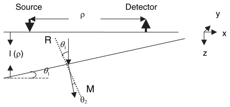
Schematic of a two-layer tissue structure with tilted interface. RM is the normal to the tilted surface, and we assume n2 > n1.
| (1) |
| (2) |
where r = (x2 + y2 + z2)1/2; Di = (1/3)(μai + μsi′)−1 are the diffusion coefficients; μai and μsi′ are the absorption and reduced scattering coefficients, respectively; and z0 = 1/(μa1 + μs1′) and Φi are the fluence rates for the layers i = 1 and 2, respectively. The modulation frequency of the source is ω = 2πf; vi is the speed of light in the medium.
The boundary conditions used are
| (3) |
| (4) |
| (5) |
| (6) |
Equation (3) refers to the extrapolated boundary condition assumed at the free surface. zb is the extrapolated distance17 given by (1 + Reff/1 − Reff)2D1. Reff depends on the refractive indices of the tissue layer and represents the fraction of photons total internally diffused at the boundary. The RI mismatch at the interface of the two layers causes discontinuity of photon fluence, for which an approximate boundary condition is given by Eq. (5). This has been shown to be valid for layers with RI mismatch up to 1.4.15 Equation (6) represents the continuity condition for the normal component of the flux at the tilted interface, expressed in terms of the tilting angle of the interface. Here θ1 represents the tilt of the interface with respect to the top surface of the tissue. From Fig. 1, we can see that θ1 also represents the angle between the direction in which the diffused light is directed and the normal to the interface. θ2 is the corresponding angle of refraction, considering the material difference between the two media with n1 and n2 being the refractive indices of layers 1 and 2, respectively.
Further, to solve diffusion equations (1) and (2) using these boundary conditions, we follow the spatial inversion approach used by Kienle et al.,5 where Eqs. (1) and (2) transform into ordinary differential equations. The boundary conditions in the spatially transformed domain corresponding to Eq. (3)–(6) are then used to solve them. The fluence rate ϕi(z, s1, s2) in the spatially transformed domain is obtained for each region in the structure at the tissue surface where
| (7) |
At the surface of the tissue, ϕ1(z, s) can be obtained by using the boundary conditions for this tilted interface structure to solve the transformed diffusion equation and is given by
| (8) |
where s2 = s12 + s22, αi2 = (Dis2 + μai + jω/vi)/Di, and ϕ = cos(θ1)/cos(θ2).
Fluence rate at the surface of the tissue (z = 0) can be obtained by spatial Fourier inversion
| (9) |
where I0 is the Bessel function of zero order and ρ is the source-detector separation. Spatial reflectance R(ρ) can be calculated as the integral of the radiance over the backward hemisphere5
| (10) |
where Rfres(θ) is the Fresnel reflection coefficient of light at an incident angle θ with respect to the normal of the boundary. It should be noted that the quantity l in the fluence rate equation is actually a function of ρ due to the tilt of the interface between the two layers and is given as l(ρ) = l0 − ρ tan(θ1), where l0 is the maximum thickness of the layer. The analysis considers only uniform tilt in any one direction. More complex analysis would be required to consider an arbitrary interface.
3. Methods
Here we discuss the numerical and computational methods followed by the experimental methods that we used to validate the solution developed in Section 2.
A. Forward and Inverse Methods
The newly developed analytical solution needs to be validated with an established method. In this section we discuss the forward simulations using the Monte Carlo method for light propagation in a two-layer tissue structure with a tilted interface and a nonlinear regression technique (inverse method) that will be used later in the paper to obtain the optical coefficients of the layered structure from measured reflectance or calculated reflectance from a two-layer tissue structure.
1. Monte Carlo Simulations
The Monte Carlo (MC) method for light propagation in layered structures was used to validate our analytical model.18–20 The layered structure is chosen as shown in Fig. 1. The general methodology used here is the same as reported in Ref. 14, except for the introduction of a tilt at the interface between the layers. In addition, time domain computation is adopted to obtain a reflectance measurement at the modulation frequency through the Fourier transform used in phantom and clinical experiments. In our simulation, 100 million photons were generated at a source location and the scattering angle was calculated using the Henyey–Greenstein function. The anisotropy factor g was chosen to be 0.9 in this simulation. The weight of this photon was decreased due to the absorption and scattering processes. For every scattering event where the calculated step size (s) (along a particular direction) caused a photon to cross the boundary between two layers, the photon was first propagated to the point where its trajectory intersected the boundary via a shortened step size (s1). When the boundary was parallel with the incident surface, the angle of incidence was computed with respect to the ±z axis and used to determine whether the photon experienced total internal reflection (from Snell's law). If the photon was internally reflected, then the z component of the photon's travel direction was reversed and the photon completed the remainder of the step (s – s1) in the same layer. Otherwise, the reflection coefficient from Fresnel's equations was computed and compared against a uniformly generated random number. If the random number was less than the reflection coefficient, the photon experienced total internal reflection; otherwise it was transmitted to the next layer. On transmission into a different layer, the final spatial location of the photon was calculated by propagating the photon with a distance of s – s1 that was adjusted in length according to the difference in total interaction coefficients between the two layers, and its direction was corrected to consider refraction by Snell's law. When the boundary is tilted, the propagation principle at the boundary is the same as the parallel boundary; however, the computation is more complex. For example, the angle of incidence, the angle of reflection, and the angle of refraction are all calculated based on the normal line of the titled interface in three dimensions. First, a plane A is established by the normal line of the titled interface and the incident photon direction. Then Snell's Law is applied to calculate the reflection or refraction angle in plane A. The calculated reflection or refraction angle is then converted to the azimuthal angle in the original (x, y, z) coordinates.
This MC simulation was performed in the time domain and the resulting data was Fourier transformed to provide amplitude and phase profiles at multiple modulation frequencies as a function of source-detector distance. A spatial resolution of 1 mm is chosen and the temporal resolution varies with the distance to the source, d. When d is less than 1 cm, between 1 and 2 cm, between 2 and 5 cm, or larger than 5 cm, the temporal resolution is chosen as 1, 3, 7, and 10 ps, respectively. The computation error in the simulation can be approximated as , where n is the number of received photons. For different temporal resolution ranges, the corresponding errors are 0.1%–0.5%, 0.5%–1.5%, 1.5%–7.0%, and 7%–15%, respectively.
2. Nonlinear Regression Method
To obtain the optical coefficients μa1, μs1′, μa2, and μs2′, a nonlinear regression method based on the Nelder–Mead simplex algorithm21,22 was used to simultaneously fit the amplitude and phase obtained from the MC simulations with the analytical solution. The Nelder–Mead simplex method is a widely used direct searching method for multidimensional unconstrained minimization. It tries to minimize a scalar-valued nonlinear function of multiple independent parameters by using only the function values. This algorithm has been previously used for estimation of tissue properties from layered tissue structure models9 and has been chosen due to its simplicity and good convergence in spite of the slow convergence rate. The thickness of the upper layer and the tilt angle are assumed to be known. In our experiments and clinical studies using the combined ultrasound and optical probe, the upper layer thickness and the interface tilting angle can be estimated with sufficient accuracy using the ultrasound image. The data collected between source-detector separations of 2.0 to 6.5 cm were used to perform the fitting. For each case, various initial values were used to avoid any local minima and to estimate the correctness of the converged value.
B. Experimental Methods
1. Phantom Experiments
The experimental validation of the analytical solution was performed using an existing frequency domain near-infrared (NIR) system. This system was a modified version of the system reported in Ref. 23. It consisted of a triwavelength laser diode source of 660, 780, and 830 nm wavelengths. The outputs of the laser diodes were amplitude modulated at 140 MHz. A single detector fiber coupled to one photomultiplier tube (PMT) detector was placed at multiple locations from 2 to 6.5 cm away from the source. Solid silicone phantoms were used to emulate the second layer over which intralipid solution was used to emulate the top layer. In phantom experiments, the layer depth and tilting angle are known, unlike in the case of clinical studies where coregistered ultrasound is used to estimate breast tissue thickness and chest-wall orientation.
2. Clinical Studies
The study protocol was approved by a local Institutional Review Board. Signed informed consent was obtained from all patients who agreed to participate in the study. In clinical experiments, NIR optical source fibers, detector fibers, and a commercial ultrasound transducer were integrated on a handheld probe.24,25 The handheld probe is circular in shape and 10 cm in diameter. Twelve dual-wavelength (780, 830 nm) laser diodes were used to sequentially illuminate the breast, and eight parallel PMT detectors were used to simultaneously detect the reflected light. Patients were scanned in a supine position while multiple sets of optical reflectance measurements were made with coregistered ultrasound images at lesion locations and symmetric locations of the contralateral normal breast. The measurements obtained at normal locations were used to estimate background optical properties, which were used to compute a weight matrix for imaging. Thus accurate estimation of background optical properties is important for improving the accuracy of tumor imaging. The geometry used for a clinical experiment is not quite the same as the configuration used in deriving the analytical solution. However, since our combined probe has 75% of the sources distributed on one side of the central ultrasound probe,25 this portion of the source-detector pair configuration approximates better the configuration used in analytical and MC simulations. The corresponding amplitude and phase profiles were used to estimate the background optical properties reported in Subsection 4.E.
The optical properties of the chest wall are not available in the literature. The only available data are the optical properties of muscles and bones. Muscle was reported to have a large absorption and medium scattering coefficients with μa in the range of 0.12 to 0.25 cm−1 and μs′ in the range of 3 to 10 cm−1.26–31 Bone is a highly absorbing and scattering medium. The reported optical properties of bone are μa = 0.23 cm−1 and μs′ = 21.4 cm−1.32,33 By assuming various ratios of muscle and bone components as representations of the chest wall, we choose optical properties of μa in the range of 0.12 to 0.23 cm−1 and μs′ in the range of 3 to 22 cm−1 in the reported studies. Throughout this paper, a range of second layer μa values was chosen for the purpose of investigating the possible effects of different types of chest-wall layers (more muscular or bony), which may vary from patient to patient.
4. Analysis and Results
In this section we first validate the analytical solution derived in Section 2 using MC simulations (in Subsection 4.A) and phantom measurements (in Subsection 4.B). In Subsection 4.C we discuss the influence of varying the tilting angle at the interface on the reflectance measured at the tissue surface. In Subsection 4.D we show the inverse calculations using the analytical solution to simultaneously obtain average optical properties of both tissue layers. In Subsection 4.E, we demonstrate the use of the analytical solution to obtain the average optical properties of breast tissue and chest-wall layers from in vivo clinical data.
A. Comparison of Analytical Solution with Monte Carlo Results
We chose a set of tissue parameters to validate our analytical results with MC simulations of two-layer tissue structures with tilted or flat interfaces and present representative cases here. A linear array of source-detector arrangements chosen was the same as that used in obtaining the analytical solution. Figures 1 and 2 show a comparison of the analytical solution and MC simulations for different second-layer absorption coefficients μa2 and reduced scattering coefficients μs2′ for both tilted and nontilted interfaces. For tilted cases, the maximum layer thickness was 2 cm (where the source is positioned), and the thickness of the layer reduces to 0.38 cm for the detector placed at 7 cm. Data were obtained from source-detector separation from 0.5 to 7 cm. Of the two cases chosen, the first case was assumed to have upper-layer properties (μa1 and μs1′) that are typically obtained from dense breast tissues and lower-layer properties, which could represent the chest-wall layer with significant bone components (relatively lower μa2 and higher μs2′). The second case has the same μa1 and μs1′ as the first case but with higher μa2 and μs2′, which could represent a chest-wall layer with significant muscle and bone components. Good agreement has been obtained for both methods. The MC calculation for case 1 with the tilted interface has used a uniform resolution of 5 ps for all source detector separations. This is because the resolution of 10 ps chosen for larger source-detector separation used for other cases seemed to be insufficient for this case with an extremely low absorption of the chest-wall layer when it is very close to the surface at larger source-detector separation (due to the tilt). Higher resolution and larger photon numbers chosen for better accuracy would result in a long computation time.
Fig. 2.
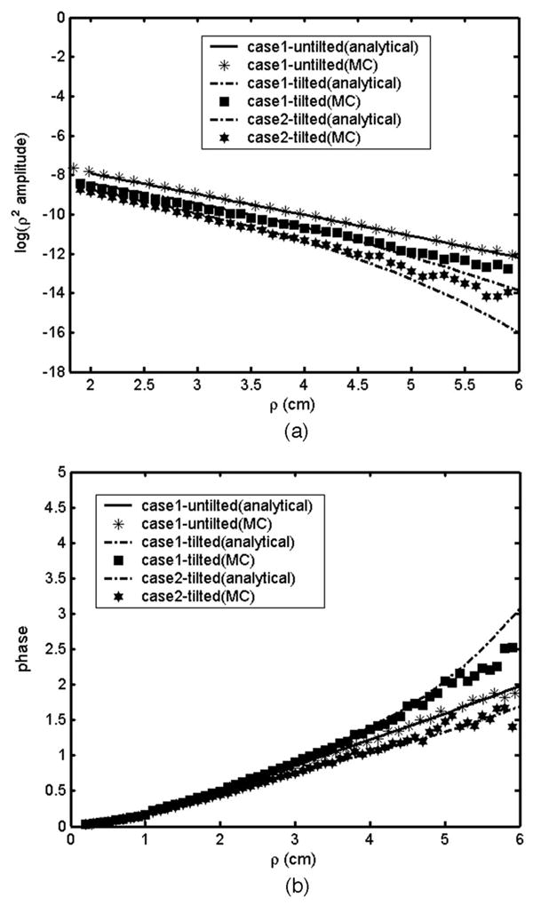
Comparison of analytical and MC calculations for a two-layer structure. (a) Amplitude plots and (b) phase plots for case 1, μa1 = 0.05 cm−1, μs1== 6 cm−1, μa2 = 0.02 cm−1, μs2== 15 cm−1, and case 2, μa1 = 0.05 cm−1, μs1= = 6 cm−1, μa2 = 0.08 cm−1, μs2== 30 cm−1. For the tilted case the first layer maximum thickness is 2 cm with a 13° tilting angle at the interface.
B. Experimental Validation of the Analytical Solution
Experimental measurements of the two-layer phantoms were made with and without tilt at the interface to validate the analytical results. The solid phantom used for the second layer had calibrated optical properties of μa = 0.01 cm−1 and μs′ = 14 cm−1 and a refractive index of 1.55. Intralipid solution was used as the top layer, thus making it easy to change the layer thickness whose refractive index is close to that of water ∼1.33. The top layer had optical properties of μa = 0.11 cm−1 and μs′ = 8.3 cm−1 and a refractive index of 1.33. Figure 3 shows the reflectance measured at 780 nm for the two-layer phantom with and without a tilted interface. In the absence of tilt, the upper layer thickness was 1.5 cm. The tilted case shown is for a tilting angle of 10° for which the layer thickness reduces to 0.35 cm for a source-detector separation of 6.5 cm. When the interface is tilted, the second layer comes closer to the tissue surface for larger source-detector separation. Here the amplitude measured at larger source-detector separation is higher for the tilted case compared with the flat interface case, mainly because of the lower absorption of the second layer (μa = 0.01 cm−1) compared to that of the first layer (μa = 0.11 cm−1). The phase measurements at larger distances increase faster for the tilted case compared with the flat interface mainly because of the higher scattering of the second layer.
Fig. 3.
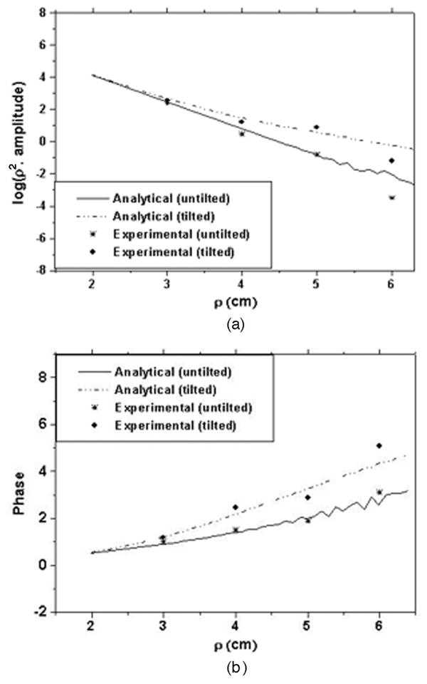
Phantom measurements compared with analytical results for tilted and nontilted interface. (a) Amplitude plots and (b) phase plots.
C. Change in Reflectance with Varying Tilt at the Interface
In this subsection we show the effect of varying the interface tilting angle on the measured reflectance obtained from a two-layer tissue structure. We have analyzed two types of layered structures. The first case has a lower and the second has a higher absorbing second layer in comparison with the absorption coefficient of the first layer. A typical case of a maximum layer thickness of 1.5 cm is chosen with varying tilting angles from 0° to 11°. Here a maximum source-detector separation of 6.5 cm is chosen for which the upper-layer thickness would be as small as 0.24 cm for an 11° tilt. In case 1, the tissue parameters chosen are close to those used in the phantom experiment, which was discussed in Subsection 3.B. From Fig. 4, we can see that when the second layer is of relatively lower absorption (case 1, μa2< μa1), the effect of tilt is more prominent on the measured reflectance phase, and when the second layer is of relatively higher absorption (case 2, μa2 > μa1), the effect of tilt is more prominent on the reflectance amplitude. This is because when the second layer is less absorbing, the light diffusing into this layer accumulates phase difference due to the longer optical path it takes, resulting in a higher phase difference when the tilting angle is larger. For a higher absorbing second layer, most of the light penetrating into this layer gets absorbed resulting in a relatively lower amplitude with increasing tilt. In this case, the major part of the detected signal is from the photons that have traveled only in the top layer, showing smaller change in a measured phase with a varying tilting angle. Thus it is important that both the amplitude and the phase data are simultaneously used for fitting while reconstructing the optical properties of a two-layer structure with a tilted interface.
Fig. 4.
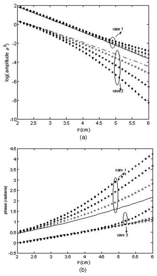
Simulated (a) amplitude and (b) phase plots for two-layer structures with varying tilting angles (circle, 4°; star, 8°; diamond, 11°) for case 1, μa1 = 0.1 cm−1, μs1== 6, μa2 = 0.01 cm−1, μs2== 14 cm−1, and case 2, μa1 = 0.05 cm−1, μs1== 6 cm−1, μa2 = 0.09 cm−1, μs2= = 14 cm−1. The dashed line and the solid line represent reflectance at zero-degree tilt for case 1 and case 2, respectively.
D. Estimation of the Optical Coefficients Using the Analytical Solution
In this subsection we use the analytical solution derived in Section 2 and nonlinear regression to estimate the two-layer tissue optical properties from the data obtained from the MC simulations. Figure 5(a) shows a plot of the estimated absorption coefficient of the first layer versus the actual absorption coefficient of the second layer, which is varied from 0.02 to 0.11 cm−1. Figure 5(b) shows the estimated absorption coefficient of the second layer versus the actual values for the same cases as in Fig. 5(a). For all the cases in Fig. 5, the absorption coefficient of the first layer is chosen as 0.05 cm−1, the reduced scattering coefficients of the first layer and the second layer are 5 and 10 cm−1, respectively. It can be seen that when the tilting effect is ignored in the estimation process, the error in calculating the absorption coefficient of the first layer increases by at least 15% and could be as large as 80% depending on the optical properties of both layers, whereas the error in estimating the absorption coefficient of the second layer is seen to increase by at least 10% and could be as high as 60% when the tilting effect is neglected. For inverse calculation neglecting the tilting effect, the first layer thickness is chosen as the average layer thickness as seen by the detection probe, which seems to yield the best results if the tilting is being ignored. Figure 6(a) shows the estimated reduced scattering coefficient of the first layer with and without considering the tilting effect versus the actual reduced scattering coefficient of the second layer, which is varied from 8 to 14 cm−1. Figure 6(b) shows the estimated reduced scattering coefficient of the second layer with and without considering tilt versus the actual reduced scattering coefficient for the cases shown in Fig. 6(a). In all the cases shown in Figs. 5 and 6, the angle of tilt is 7° and the maximum thickness of the first layer is 1.2 cm, which would reduce to 0.34 cm for the maximum source-detector separation at 7 cm. It can be seen that, in comparison to the inverse calculation considering the tilting effect at the interface, the error in estimating the scattering coefficient of the first layer increases by at least 8% and could be as high as 20% when the effect of tilt is neglected, whereas the error in estimating the second-layer reduced scattering coefficient increases by at least 15% and could be as high as 40% when the effect of tilt is ignored. The data obtained at source-detector separations above 2 cm is used for fitting. The first-layer absorption coefficient is usually obtained accurately when the tilt is considered and with a higher estimation error when the tilting effect is ignored. The error is larger for the cases when the absorption or reduced scattering coefficient of the second layer is relatively lower.
Fig. 5.
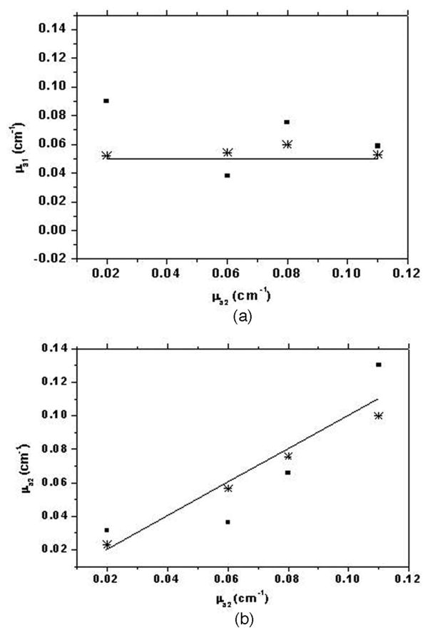
Estimated absorption coefficient of (a) the first layer (μa1) and (b) the second layer (μa2) determined by nonlinear regression of the analytical solution to MC data plotted versus the true value of the absorption coefficient of the second layer (μa2). Parameters chosen for MC simulations are a maximum layer thickness of 1.2 cm, an interface tilt of 7°, μa1 = 0.05 cm−1, μs1== 5 cm−1, μs2== 10 cm−1, and μa2 varying from 0.02 to 0.11 cm−1. The solid line indicates the true value, stars represent the estimated values considering the interface tilt, and squares represent the estimated values ignoring the interface tilt.
Fig. 6.
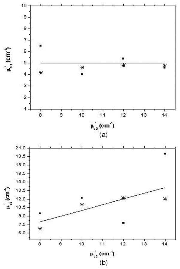
Estimated reduced scattering coefficient of (a) the first layer (μs1=) and (b) the second layer (μs2=) determined by nonlinear regression of the analytical solution to MC data plotted versus the true value of reduced scattering coefficient of the second layer (μs2=). Parameters chosen for MC simulations are a maximum layer thickness of 1.2 cm, an interface tilt of 7°, μa1 = 0.05 cm−1, μs1== 5 cm−1, μa2 = 0.08 cm−1, and μs2=varying from8 to 14 cm−1. The solid line indicates the true value, stars represent the estimated values considering the interface tilt, and squares represent the estimated values ignoring the interface tilt.
Estimation error in the scattering coefficient of the second layer is less than 20% and that of the absorption coefficient is less than 15% when the tilting effect is considered. We have noticed that these percentages may vary slightly, with one of the coefficients estimated with higher accuracy, whereas the accuracy of the other coefficient is reduced.
E. Use of the Analytical Solution to Estimate Average Tissue Optical Properties From Clinical Data
In this subsection we show the use of the two-layer model to estimate the background tissue optical properties from clinical data. We present the inverse calculations to the data obtained from one 52-year-old patient and another 21-year-old patient under study. Figure 7 shows an ultrasound image obtained from the normal breast of the first patient. The breast tissue thickness is about 1.25 cm, and the data collected from both wavelengths were used to obtain the optical properties of the breast tissue and the chest-wall layer at 780 and 830 nm. Table 1 shows the estimated average optical properties of the breast tissue (μa1 and μs1′) and those of the chest wall (μa2 and μs2′). The optical properties were reasonable and consistent at both wavelengths. Figure 8 shows the ultrasound image obtained from the second patient in which the tilted chest wall can be seen clearly. The tilt is about 6° with a maximum breast tissue layer thickness of 1.75 cm reducing to as small as 1 cm.
Fig. 7.
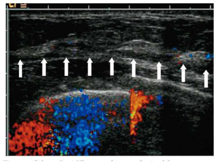
(Color online) Ultrasound image obtained from a 52-year-old patient with an effective breast tissue thickness of 1.25 cm at the breast tissue–chest wall interface marked by the array of white arrows.
Table 1. Estimated Background Absorption and Reduced Scattering Coefficient of Breast Tissue and Chest Walla.
| Measurement λ | μa1 (cm−1) | μs1= (cm−1) | μa2 (cm−1) | μs2 (cm−1) |
|---|---|---|---|---|
| 780 nm | 0.0797 | 4.21 | 0.182 | 17.66 |
| 830 nm | 0.070 | 4.07 | 0.179 | 18.31 |
Taken from the optical reflectance measurement of the first patient with the corresponding ultrasound image shown in Fig. 7.
Fig. 8.
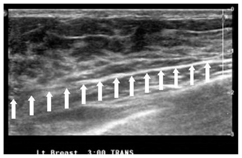
Ultrasound image obtained from a 21-year-old patient showing a maximum breast tissue thickness of about 1.75 cm reducing to 1 cm with a tilt angle of 6°. The breast tissue–chest wall interface is marked by the array of white arrows. The horizontal scale is 6.5 cm.
Table 2 shows the average optical properties estimated from measurements using the average layer thickness of 1.4 cm with the tilting angle ignored, whereas Table 3 shows the average properties estimated by using the measured 6° tilt. It is interesting to note that after considering the tilt, the average absorption and reduced scattering coefficients seem to follow the general trend that we have observed from many normal breasts: The average absorption coefficient measured at 830 nm is in general higher than that obtained at 780 nm, but the reduced scattering coefficient is in general lower than that obtained at 780 nm.
Table 2. Estimated Background Absorption and Reduced Scattering Coefficient of Breast Tissue and Chest Walla.
| Measurement λ | μa1 (cm−1) | μs1 (cm−1) | μa2 (cm−1) | μs2 (cm−1) |
|---|---|---|---|---|
| 780 nm | 0.0426 | 9.799 | 0.0768 | 15.556 |
| 830 nm | 0.0420 | 10.04 | 0.0799 | 11.578 |
Taken from the optical reflectance measurement of the second patient with the corresponding ultrasound image shown in Fig. 8. The results shown are from using an average layer thickness of 1.4 cm.
Table 3. Estimated Background Absorption and Reduced Scattering Coefficient of Breast Tissue and Chest Walla.
| Measurement λ | μa1 (cm−1) | μs1 (cm−1) | μa2 (cm−1) | μs2 (cm−1) |
|---|---|---|---|---|
| 780 nm | 0.052 | 9.75 | 0.079 | 12.4 |
| 830 nm | 0.073 | 6.8 | 0.13 | 9.93 |
Taken from the optical reflectance measurement of the second patient with the corresponding ultrasound image shown in Fig. 8. The results shown are from using measured tilt from the ultrasound image.
5. Discussion and Summary
We have developed an analytical solution for light propagation in two-layered tissue structures with a tilted interface and validated it using MC calculations and phantom experiments with good agreement in the results. Using this solution, we have analyzed the effect of varying the interface tilting angle on the reflectance measurements of two-layer structures. We have observed that the effect of tilt results in increased deviation in phase or amplitude measurements as compared to the nontilted case depending on whether the lower layer has lower or higher optical absorption. A nonlinear regression method has been used to estimate the two-layer optical properties from the MC data. Our results show that ignoring the tilting effect could result in errors in the estimation of optical properties of both tissue layers. For the typical cases that we considered, where the maximum upper layer thickness was about 1.5 cm or less, we have observed higher errors in the estimation of the upper-layer optical properties when the tilt is ignored. This could be crucial in imaging smaller breasts where the chest-wall interface may be tilted with respect to the measurement probe.
Coregistered ultrasound images can provide the breast–chest interface depth and titling angle in real time. The probe geometry used to collect data was not exactly the same as the geometry used in deriving the analytical solution, but the consistent background optical properties obtained from two optical wavelengths from each patient indicate the robustness of the two-layer model and the nonlinear regression method. Further studies are planned to obtain more data sets from selected patients with smaller breasts at multiple locations of different breast tissue–chest wall orientations to validate the technique. With the better accuracy in estimating tissue background optical properties for two-layer structures with tilted interfaces, the next step is to develop robust image reconstruction algorithms using either an analytical solution or a numerical method for the layered medium. Currently, we are working in this direction.
Acknowledgments
This work was supported by the National Institutes of Health (grant R01EB002136) and the Army Medical Research and Materiel Command (grant 81XWH-05-1-0299).
References
- 1.Fishkin JB, Coquoz O, Anderson ER, Brenner M, Tromberg BJ. Frequency-domain photon migration measurements of normal and malignant tissue optical properties in a human subject. Appl Opt. 1997;36:10–20. doi: 10.1364/ao.36.000010. [DOI] [PubMed] [Google Scholar]
- 2.Tromberg B, Shah N, Lanning R, Cerussi A, Espinoza J, Pham T, Svaasand L, Butler J. Noninvasive in vivo characterization of breast tumors using photon migration spectros-copy. Neoplasia. 2000;2:26–40. doi: 10.1038/sj.neo.7900082. [DOI] [PMC free article] [PubMed] [Google Scholar]
- 3.Kienle A, Lilge L, Patterson MS, Hibst R, Steiner R, Wilson BC. Spatially resolved absolute diffuse reflectance measurements for noninvasive determination of optical scattering and absorption coefficients of biological tissue. Appl Opt. 1996;35:2304–2314. doi: 10.1364/AO.35.002304. [DOI] [PubMed] [Google Scholar]
- 4.Zhu Q, Chen N, Kurtzman S. Imaging tumor angiogenesis by use of combined near-infrared diffusive light and ultrasound. Opt Lett. 2003;28:337–339. doi: 10.1364/ol.28.000337. [DOI] [PMC free article] [PubMed] [Google Scholar]
- 5.Kienle A, Patterson MS, Dögnitz N, Bays R, Wagnièrese G, Bergh H. Noninvasive determination of the optical properties of two-layered turbid media. Appl Opt. 1998;37:779–791. doi: 10.1364/ao.37.000779. [DOI] [PubMed] [Google Scholar]
- 6.Dayan I, Havlin S, Weiss GH. Photon migration in a two-layer turbid medium. A diffusion analysis. J Mod Opt. 1992;39:1567–1582. [Google Scholar]
- 7.Fawzi YS, Youssef AM, El-Batanony MH, Kadah YM. Determination of optical properties of a two-layer tissue model by detecting photons migrating at progressively increasing depth. Appl Opt. 2003;42:6398–6411. doi: 10.1364/ao.42.006398. [DOI] [PubMed] [Google Scholar]
- 8.Farrel TJ, Patterson MS, Essenpreis M. Influence of layered tissue architecture on estimates of tissue optical properties obtained from spatially resolved diffuse reflectometry. Appl Opt. 1998;37:1958–1972. doi: 10.1364/ao.37.001958. [DOI] [PubMed] [Google Scholar]
- 9.Pham TH, Spott T, Svaasand LO, Tromberg BJ. Quantifying the properties of two-layer turbid media with frequency-domain diffuse reflectance. Appl Opt. 2000;39:4733–4745. doi: 10.1364/ao.39.004733. [DOI] [PubMed] [Google Scholar]
- 10.Alexandrakis G, Farrell TJ, Patterson MJ. Accuracy of diffusion approximation in determining the optical properties of a two-layer turbid medium. Appl Opt. 1998;37:7401–7409. doi: 10.1364/ao.37.007401. [DOI] [PubMed] [Google Scholar]
- 11.Martelli F, Bianco SD, Zaccanti G. Procedure for retrieving the optical properties of a two-layered medium from time-resolved reflectance measurements. Opt Lett. 2003;28:1236–1238. doi: 10.1364/ol.28.001236. [DOI] [PubMed] [Google Scholar]
- 12.Tualle JM, Prat J, Tinet E, Avrillier S. Real-space Green's function calculation for the solution of the diffusion equation in stratified turbid media. J Opt Soc Am A. 2000;17:2046–2055. doi: 10.1364/josaa.17.002046. [DOI] [PubMed] [Google Scholar]
- 13.Huang M, Zhu Q. A two-layer model for NIR breast imaging with the assistance of ultrasound. Proc SPIE. 2005;5693:121–128. [Google Scholar]
- 14.Xu C, Zhu Q. Estimation of chest-wall-induced diffused wave distortion with assistance of ultrasound. Appl Opt. 2005;44:4255–4264. doi: 10.1364/ao.44.004255. [DOI] [PMC free article] [PubMed] [Google Scholar]
- 15.Martelli F, Bianco SD, Zaccanti G. Effect of the refractive index mismatch on light propagation through diffusive layered media. Phys Rev E. 2004;70:011907. doi: 10.1103/PhysRevE.70.011907. [DOI] [PubMed] [Google Scholar]
- 16.Deghani H, Brooksby B, Vishwanath K, Pogue BW, Paulsen K. The effects of internal refractive index variation in near-infrared optical tomography: a finite element modeling approach. Phys Med Biol. 2003;48:2713–2727. doi: 10.1088/0031-9155/48/16/310. [DOI] [PubMed] [Google Scholar]
- 17.Haskell RC, Svaasand LO, Tsay TT, Feng TC, McAdams M, Tromberg BJ. Boundary conditions for the diffusion equation in radiative transfer. J Opt Soc Am A. 1994;11:2727–2741. doi: 10.1364/josaa.11.002727. [DOI] [PubMed] [Google Scholar]
- 18.Flock ST, Patterson MS, Wilson BC, Wyman DR. Monte Carlo modeling of light-propagation in highly scattering tissues. I. Model predictions and comparison with diffusion theory. IEEE Trans Biomed Eng. 1989;36:1162–1168. doi: 10.1109/tbme.1989.1173624. [DOI] [PubMed] [Google Scholar]
- 19.Wang L, Jacques SL, Zheng L. MCML-Monte Carlo modeling of light trasport in multilayered tissues. Comput Methods Programs Biomed. 1995;47:131–146. doi: 10.1016/0169-2607(95)01640-f. [DOI] [PubMed] [Google Scholar]
- 20.Boas D, Culver J, Stott J, Dunn A. Three-dimensional Monte Carlo code for photon migration through complex heterogeneous media including the adult human head. Opt Express. 2002;10:159–170. doi: 10.1364/oe.10.000159. [DOI] [PubMed] [Google Scholar]
- 21.Press WH, Flannery BP, Teukolsky SA, Vettering WT. Numerical Recipes in C. Cambridge U Press; 1988. [Google Scholar]
- 22.Lagarias JC, Reeds JA, Wright MH, Wright PE. Convergence properties of the Nelder–Mead sinplex method in low dimensions. SIAM J Optim. 1998;9:112–147. [Google Scholar]
- 23.Chen NG, Guo P, Yan S, Piao D, Zhu Q. Simultaneous near infrared diffusive light and ultrasound imaging. Appl Opt. 2001;40:6367–6280. doi: 10.1364/ao.40.006367. [DOI] [PMC free article] [PubMed] [Google Scholar]
- 24.Zhu Q, Cronin E, Currier A, Vine HS, Huang M, Chen NG, Xu C. Benign versus malignant breast masses: optical differentiation using US to guide optical imaging reconstruction. Radiology. 2005;237:57–66. doi: 10.1148/radiol.2371041236. [DOI] [PMC free article] [PubMed] [Google Scholar]
- 25.Zhu Q, Kurtzman S, Hegde P, Tannenbaum S, Kane M, Huang M, Chen NG, Jagjivan B, Zarfos K. Utilizing optical tomography with ultrasound localization to image heterogeneous hemoglobin distribution in large breast cancers. Neoplasia. 2005;7:263–270. doi: 10.1593/neo.04526. [DOI] [PMC free article] [PubMed] [Google Scholar]
- 26.Cheong W, Prahl SA, Welch AJ. A review of the optical property of biological tissues. IEEE J Quantum Electron. 1990;26:2166–2185. [Google Scholar]
- 27.Patterson MS, Chance B, Wilson BC. Time resolved reflectance and transmittance for the noninvasive measurement of tissue optical properties. Appl Opt. 1989;28:2331–2336. doi: 10.1364/AO.28.002331. [DOI] [PubMed] [Google Scholar]
- 28.Wilson BC, Patterson MS, Flock ST, Moulton JD. The optical absorption and scattering properties of tissues in the visible and near-infrared wavelength range. In: Douglas RH, Moan J, Doll'Acqua F, editors. Light in Biology and Medicine. Vol. 1. Plenum: 1988. pp. 45–52. [Google Scholar]
- 29.Martelli F, Del Bianco S, Zaccanti G, Pifferi A, Torricelli A, Bassi A, Taroni P, Cubeddu R. Phantom validation and in vivo application of an inversion procedure for retrieving the optical properties of diffusive layered media from time-resolved reflectance measurements. Opt Lett. 2004;29:2037–2039. doi: 10.1364/ol.29.002037. [DOI] [PubMed] [Google Scholar]
- 30.Matcher SJ, Cope M, Delpy DT. In vivo measurements of the wavelength dependence of tissue-scattering coefficients between 760 and 900 nm measured with time-resolved spectroscopy. Appl Opt. 1997;36:386–396. doi: 10.1364/ao.36.000386. [DOI] [PubMed] [Google Scholar]
- 31.Srinivasan R, Kumar D, Singh M. Optical tissue-equivalent phantoms for medical imaging. Trends Biomater Artif Organs. 2002;15:42–47. [Google Scholar]
- 32.Xu Y, Iftimia N, Jiang H, Key LL, Bolster MB. Imaging of in vitro and in vivo bones and joints with continuous-wave diffuse optical tomography. Opt Express. 2001;8:447–451. doi: 10.1364/oe.8.000447. [DOI] [PubMed] [Google Scholar]
- 33.Firbank M, Hiraoka M, Essenpreis M, Delpy DT. Measurement of the optical properties of the skull in the wavelength range 650–950 nm. Phys Med Biol. 1993;38:503–510. doi: 10.1088/0031-9155/38/4/002. [DOI] [PubMed] [Google Scholar]