Sensitivity analysis for causal inference using inverse probability weighting

Abstract

Evaluation of impact of potential uncontrolled confounding is an important component for causal inference based on observational studies. In this article, we introduce a general framework of sensitivity analysis that is based on inverse probability weighting. We propose a general methodology that allows both non-parametric and parametric analyses, which are driven by two parameters that govern the magnitude of the variation of the multiplicative errors of the propensity score and their correlations with the potential outcomes. We also introduce a specific parametric model that offers a mechanistic view on how the uncontrolled confounding may bias the inference through these parameters. Our method can be readily applied to both binary and continuous outcomes and depends on the covariates only through the propensity score that can be estimated by any parametric or non-parametric method. We illustrate our method with two medical data sets.

1 Introduction

When the treatment assignment is not randomized, as in most observational studies, bias may be introduced in causal inference when pre-treatment covariates associated with treatment assignment and the outcome are not properly adjusted. This is particularly critical for inference based on large data sets (i.e. electronic medical record databases) where precision can be rather high, and thus the accuracy of the estimator is dominated by the bias. The potential outcome model has been established as a major theoretical framework that underlies most of the available methods for causal inference including matching covariates (Cochran, 1953; Rubin, 1973), outcome regression, methods based on propensity scores (Rosenbaum and Rubin, 1983b; Rubin and Thomas, 1996) and double-robust estimator (Bang and Robins, 2005). The key idea of the potential outcome model is that for each unit, there is a potential outcome under each treatment and assessment of the causal effect involves comparison of these potential outcomes (Holland, 1986). Since not all of the potential outcomes are observed for each unit in empirical data, causal inference can also be viewed as a missing-data problem (Rubin, 1978).

Common to many methods in observational studies is the assumption of “no uncontrolled confounding”, which states that conditional on the pre-treatment covariates included in the analysis, the treatment assignment and potential outcome are independent. Such an assumption serves as the basis for the large volume of research articles on different methods for bias correction and efficiency improvement. However, it is also of great practical interest to examine the extent to which the inference is sensitive to violation of this assumption. It is well known that it is not possible to test the assumption of no uncontrolled confounding using observed data. Therefore, sensitivity analysis is an important component for proper interpretation of the data and accurate statement of the conclusion when assessing causal effects using observational data. The general strategy in sensitivity analysis involves postulation of various assumptions on the nature of the associations of the uncontrolled confounders with treatment assignment and outcomes, followed by examination of the bias induced. Usually, these assumptions are in the format of plausible values of parameters not identifiable from the observed data that characterize those associations. These parameters will be referred to as non-estimable parameters in this article.

Compared with methods assuming no uncontrolled confounding, sensitivity analysis has been relatively sparse in the literature. Rosenbaum (1995) developed a logistic model in the randomization-based framework, where a single parameter measuring the strength of association between the missed covariate and treatment assignment conditional on covariates already included is linked to a minimum and a maximum p-values of the inference. The p-values under different values of this parameter allow one to assess the sensitivity to uncontrolled confounding. Rosenbaum and Rubin (1983a) proposed an approach for binary outcome with one categorical covariate, where the sensitivity of the estimate to different values of non-estimable parameters (due to unobserved covariates) in the full likelihood function was examined. The same authors also examined the bias due to incomplete matching (Rosenbaum and Rubin, 1985). Brumback et al. (2004) developed an approach where the mean difference between treatment groups within each covariate stratum is used to examine the impact of residual confounding, which uses a similar type of strategy reported previously (Cole et al., 2005; Ko et al., 2003; Robins, 1999). Lin et al. (1998) studied bias induced by uncontrolled confounding in the parametric regression setting. It was shown that under certain conditions there exists a simple algebraic relationship between the true effect and the “apparent” effect when there is uncontrolled confounding – see Hernan and Robins (1999) for more discussions. MacLehose et al. (2005) and Kuroki and Cai (2008) proposed linear programming methods to derive the upper and lower bounds for the causal effect on a binary outcome. Greenland (2005) developed a general Bayes framework to correct bias due to confounding, missing data, and classification error by including a bias model with relevant bias parameters. Other methods include Arah et al. (2008), Copas and Li (1997), Imbens (2003), Sturmer et al. (2007a,b).

In this article, we propose a general framework for sensitivity analysis of inference based on inverse probability weighting (IPW) that supports both parametric and non-parametric modeling of the probability of treatment assignment (propensity score). We also propose a specific type of parametric model along the same line that provides a more mechanistic view on how the uncontrolled confounding may bias the inference. The parametric model also provides guidance on how to postulate the non-estimable parameters when the association of uncontrolled confounders with treatment assignment is entirely unstructured. Our method generates upper and lower bounds for the causal effect under fixed values of two non-estimable parameters that characterize the error in the estimated propensity score due to uncontrolled confounding and its correlation with the potential outcome. The advantages of our method over previously published methods include: (i) it can be used for both continuous and binary outcomes; (ii) it involves the covariates only through the propensity score and therefore many covariates can be included; (iii) the sensitivity analysis is driven by only two parameters with sensible scales; (iv) the propensity score can be estimated from any parametric or non-parametric method under the general framework; and (v) the parametric model provides insight on the process that induces biases. In particular, property (ii) allows our method to deal with high-dimensional propensity score model, which is difficult to implement in previous method (e.g. Brumback et al., 2004). A limitation of our method is that the assumption is based on potential outcomes instead of observed outcomes (Vander Weele, 2008), which make it less intuitively appealing. Nevertheless, our method is set up in a very general framework that can be applied to most practical applications. In Section 2, we introduce some notations and describe our method. We illustrate our method with two application examples in Section 3. We conclude the article with a discussion in Section 4.

2 Method

2.1 Background

Our method is built on the potential outcome framework for two-level treatment (treated versus control) (Holland, 1986; Rubin, 1974, 1978, 2005). Let Y₁ and Y₀ be the potential outcomes when there is treatment or not, respectively. The principle idea of causal inference based on the potential outcomes is that the causal effect is captured by some kind of contrast between Y₁ and Y₀ (e.g. Y₁−Y₀). As in many practical problems, we only observe one of the two potential outcomes, direct estimation of the causal effect at individual level is not possible. Most of the causal inference problems focus on the estimation of the average treatment effect (ATE) for a target population, that is, Δ = E(Y₁)−E(Y₀). In observational studies, because of the non-randomness of treatment assignment, difference in the sample means between the two treatment arms would be a biased estimator of ATE. One of the approaches to eliminate the potential bias is called IPW estimation (Hirano and Imbens, 2001; Robins et al., 1994). For the IPW method, each unit has a probability of being assigned to the treatment arm that depends on certain baseline characteristics. This probability is also called the propensity score (Rosenbaum and Rubin, 1983b). The basic idea of IPW is to calculate the difference in the weighted sample means between the two arms with the weight being the inverse of the propensity score (for treated units) or one minus the propensity score (for control units). To be specific, let Z be the treatment indicator such that Z = 1 means treated and 0 means control. Therefore, Y=ZY₁+(1−Z)Y₀ is the observed outcome. We denote by X the observed covariate vector and S = E(Z|X) the propensity score. Under the assumption of no uncontrolled confounding (weak ignorability) (Rubin, 2005), Y_k ∐ Z|X for k = 0,1 (here ∐ means independent), the following equations have been well established (Hirano and Imbens, 2001):

$$E\left(Y_1\right)-E\left(Y_0\right)=E\left(\frac{YZ}{S}\right)-E\left(Y_0\right)=E\left(\frac{YZ}{S}\right)-E\left(\frac{Y\left(1-Z\right)}{1-S}\right),0<S<1.$$ (1)

Equation (1) is the basis for the unbiased estimation of the marginal mean of the outcome under each treatment level and the causal effect using IPW. The intuitive explanation of Eq. (1) can be best understood through the concept of pseudo-population. For instance, each unit with Z = 1 has a probability of S to be assigned to the treatment. Therefore, in terms of the distribution of Y₁, a pseudo-population where such a unit is duplicated 1/S times represents the original population from which the unit is sampled. The mean of Y₁ for the two populations then should be the same.

2.2 A general framework for sensitivity analysis

When there is uncontrolled confounding, Y_k (k = 0,1) and Z are not independent conditional on X. We assume that Y_k ∐Z|(X,X*) (k = 0,1), where X* is a vector of covariates that are either not observed or not included in the analysis. Although S is still a conditional probability, it will not be equal to the true propensity score S^*=E(Z|X,X^*) with probability 1. From now on, we will call S the pseudo-propensity score to distinguish it from S^*. The basic idea of our method is to develop bounds of the causal effect (or marginal means if those are of interest) by accounting for the error in using S to approximate S^*. The bounds will allow us to assess the sensitivity of the result to uncontrolled confounding.

We denote by ε₁ = S^*/S (0<ε₁<∞) the multiplicative error of S with respect to S^*. Here, ε₁ is a measure of the quality of the pseudo-propensity score in approximating the true propensity score. The variance of ε₁ is a measure of the overall deviation of S from S^* with larger variance indicating more deviation. The relationship between S and S^* can be characterized by

$$S=E(S^{\ast }|S),$$ (2)

where the expectation is with respect to the distribution of (X,X^*) within a pseudo-propensity score stratum with value S. To see this, note that

$$S=E\left(\text{Z}|\text{X}\right)=E\left[E\left(\text{Z}|\text{X},{\text{X}}^{\ast }\right)|\text{X}\right]=E\left(S^{\ast }|\text{X}\right)\Rightarrow E\left(S^{\ast }|S\right)=S.$$

Equation (2) says that S^* will center at S within each stratum of S. It also implies by the law of iterated expectation and decomposition of variance that

$$E\left({\epsilon }_1\right)=E\left(\frac{E\left(S^{\ast }|S\right)}{S}\right)=1,\text{Var}\left({\epsilon }_1\right)=\text{Var}\left(\frac{E\left(S^{\ast }|S\right)}{S}\right)+E\left(\frac{\text{Var}\left(S^{\ast }|S\right)}{S^2}\right)=E\left(\frac{\text{Var}\left(S^{\ast }|S\right)}{S^2}\right).$$

Since S is not the true propensity score when there is uncontrolled confounding, the IPW based on S may be biased. As an example, consider the assessment of the magnitude of bias in estimating the mean of Y₁. First, we observe that

$$E\left(\frac{YZ}{S}\right)=E\left(\frac{Y_{1}Z}{S}\right)=E\left(E\left(\frac{Y_{1}Z}{S}|\left(\text{X},{\text{X}}^{\ast },Y_1\right)\right)\right)=E\left(\frac{Y_{1}E\left(Z|\text{X},{\text{X}}^{\ast },Y_1\right)}{S}\right)=E\left(\frac{Y_1{S}^{\ast }}{S}\right)=E\left(Y_1{\epsilon }_1\right),$$

where the fourth equality is due to the independence of Z and Y₁ conditional on (X,X^*). Then we have

$$E\left(\frac{YZ}{S}\right)-E\left(Y_1\right)=E\left(Y_1{\epsilon }_1\right)-E\left({\epsilon }_1\right)E\left(Y_1\right)={\text{ρ}}_1{\left[\text{Var}\left(Y_1\right)\text{Var}\left({\epsilon }_1\right)\right]}^{1/2}.$$ (3)

Here, ρ₁ is the correlation coefficient between Y₁ and ε₁. Equation (3) represents the key idea of our method. It says that the bias of YZ/S in estimating E(Y₁) is governed by two non-estimable quantities in addition to the variance of Y₁ (also non-estimable), the correlation between the multiplicative error ε₁ in propensity score due to uncontrolled confounders and the potential outcome Y₁, and the variance of ε₁. The first quantity, in some sense, characterizes the strength of the association between the missed confounders and the potential outcome. It can be interpreted as a measure that captures the concordance between the outcome value and the amount of extra weight assigned to the outcome value due to uncontrolled confounders. The second quantity, as seen later in the parametric model, characterizes the strength of the association between the missed confounders and the treatment assignment. Stronger correlation and higher variation in ε₁ will lead to higher bias. Intuitively, since higher ε₁ means that S severely under-estimates S^*, a positive correlation implies that higher Y₁ values are over-duplicated, whereas lower Y₁ values are under-duplicated in the pseudo-population. Therefore, the IPW based on S over-estimates E(Y₁). Similarly, a negative correlation implies an under-estimate of E(Y₁). On the other hand, the variance of ε₁ characterizes the quality of S and higher value of the variance indicates more severe deviation from S^* and therefore more bias in estimating E(Y₁).

2.2.1 Continuous outcome

To derive the bounds for marginal means and the causal effect, we will assume that Y₁,Y₀ ∈[0,1]. As in most practical problems continuous outcomes can be monotonically transformed to the unit interval based on conservative estimates of the range of the outcomes, this assumption has quite general applicability.

We first introduce some notations. Let $E\left(YZ/S\right)={\text{θ}}_1$, $E\left(Y_1|Z=1\right)={\text{μ}}_1$, $E\left(Y_1^2|Z=1\right)={\text{η}}_1$, $E\left(Y_1|Z=0\right)={\text{μ}}_0$, $E\left(Y_1^2|Z=0\right)={\text{η}}_0$, $E\left(Z\right)=\text{π}$, and $\text{Var}\left({\epsilon }_1\right)={\text{ν}}_1$. Then

$$\text{Var}(Y_1)=E(Y_1^2)-{[E(Y_1)]}^2=\pi {\eta }_1+(1-\pi ){\eta }_0-{[E(Y_1)]}^2$$ (4)

Since Y₁ ∈ [0,1], it is easy to show that ${\text{μ}}_0^2\le {\text{η}}_0\le {\text{μ}}_0$. Because μ₀=(E(Y₁)–πμ₁)/(1−π), we can replace η₀ in (4) by the expression of its bounds. After some algebra, we have

$$\text{ψ}[E\left(Y_1\right)(E\left(Y_1\right)-2{\text{μ}}_1)+d]\le \text{Var}\left(Y_1\right)\le E\left(Y_1\right)\left(1-E\left(Y_1\right)\right)-b,$$ (5)

where ψ= π/(1−π), b = π(μ₁−η₁), and $d=\text{π}{\text{μ}}_1^2+\left(1-\text{π}\right){\text{η}}_1$ are all estimable quantities. Hence, in consideration of Eq. (3) and the inequalities above, we have

$${\text{ρ}}_1^2{\text{ν}}_1\text{ψ}\left[E\left(Y_1\right)\left(E\left(Y_1\right)-2{\text{μ}}_1\right)+d\right]\le {\left({\text{θ}}_1-E\left(Y_1\right)\right)}^2\le {\text{ρ}}_1^2{\text{ν}}_1\left[E\left(Y_1\right)\left(1-E\left(Y_1\right)\right)-b\right]$$ (6)

The region defined by inequalities (6) includes two intervals, one for positive ρ₁ and one for negative ρ₁ We will call the interval that corresponds to the intended sign of ρ₁ the feasible region of E(Y₁). In Fig. 1, we illustrate the idea through a geometric demonstration. Essentially, Fig. 1 shows that the feasible region for E(Y₁) is determined by the positions and shapes of three second-order polynomials. The distances between θ₁ and the two shaded regions on the X-axis represent possible magnitude of bias depending on the sign of ρ₁ The width of the interval originates from uncertainty on the relationship between E(Y₁) and Var(Y₁). Note that inequalities in (6) involve non-estimable parameters (ρ₁,ν₁). For any given (ρ₁,ν₁), one can solve the equations in (6) to obtain the lower (l₁) and upper (L₁) limits of the interval. These limits set the boundaries for E(Y₁) after adjusting for the error in estimating the propensity score (ν₁) and its correlation with the potential outcome (ρ₁) By examining l₁ and L₁ under different values of (ρ₁,ν₁), one can gain insight on the robustness of the estimate of E(Y₁).

Figure 1.

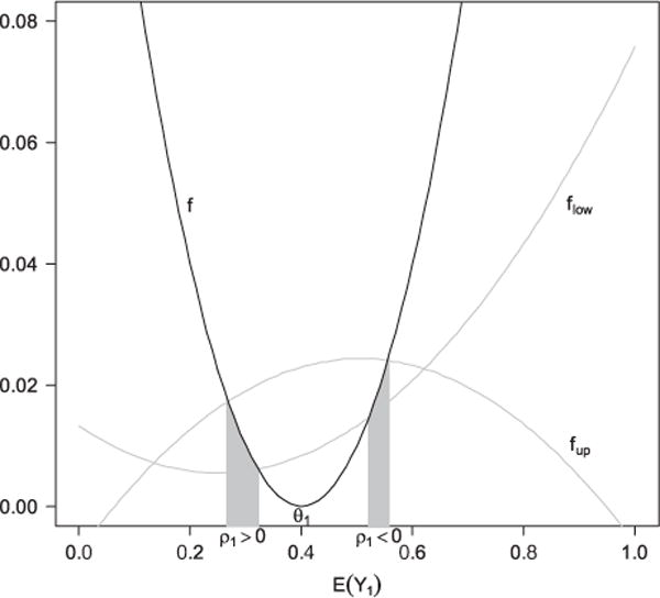
Illustration of the feasible regions of E(Y₁) defined by formula (6). f_low, f, and f_up can be viewed as three functions of E(Y₁) that correspond to the three terms in (6): $f_{\text{low}}={\text{ρ}}_1^2{\text{ν}}_1\text{ψ}\left[E\right(Y_1\left)\right(E\left(Y_1\right)-2{\text{μ}}_1)+d]$, $f={({\text{θ}}_1-E(Y_1\left)\right)}^2$, $f_{\text{up}}={\text{ρ}}_1^2{\text{ν}}_1\left[E\right(Y_1\left)\right(1-E\left(Y_1\right))-b]$.The two intervals on X-axis under the gray regions correspond to the feasible regions under ρ₁>0 and ρ₁<0, respectively. Here, θ₁= 0.4, |ρ₁| = 0.5, π = 0.5, ν₁ = 0.5, μ₁ = 0.25, ψ= 1, η₁ = 0.15, b = 0.05, and d = 0.10625.

The same type of bounds l₀ and L₀ can also be derived for E(Y₀) for a fixed pair of (ρ₀,ν₀), where ν₀ is the variance of ε₀ = (1−S^*)/(1−S) and ρ₀ is the correlation coefficient of Y₀ and ε₀.

As the correlation coefficient is a popular and sensible measure to most users, the variance of the error term might not be sensible enough to be specified easily. Since a random variable taking values in the unit interval with mean μ has the maximum variance of μ(1−μ)(Var(Y) = E(Y²)−[E(Y)]² ≤ E(Y) − [E(Y)]² = μ(1−μ)), we have

$${\text{ν}}_1=\text{Var}\left({\epsilon }_1\right)=E\left(\frac{\text{Var}\left(S^{\ast }|S\right)}{S^2}\right)\le E\left(\frac{S\left(1-S\right)}{S^2}\right)=E\left(\frac{1-S}{S}\right)={\text{ν}}_1.$$

Therefore, instead of proposing a value of ν₁, we can postulate the percentage of the maximum possible variance λ₁= ν₁/V₁. Similarly, we can propose λ₀=v₀/V₀, where V₀ = E(S/(1S)).

2.2.2 Binary outcome

When the outcome is binary, the right-hand side inequality in (5) becomes

$${({\text{θ}}_1-E(Y_1\left)\right)}^2={\text{ρ}}_1^2{\text{ν}}_{1}E\left(Y_1\right)(1-E(Y_1\left)\right).$$ (7)

For any fixed (ρ₁,ν₁), the region defined by (6), if exists, is a point. Therefore, l₁= L₁. Similarly, l₀ = L₀.

2.2.3 Bounds for average treatment effect

It is obvious that l₁−L₀ and L₁−l₀ are a set of lower and upper bounds for the causal effect. In practice, a propensity score model is first fitted to the data and the estimated propensity score will play the role of pseudo-propensity score. The lower and upper limits are then derived using parameters from the empirical distributions. It often provides sufficient insight into the robustness of the result by setting |ρ₁| = |ρ₀| ⁼ ρ and λ₁= λ₀=λ (as long as λ₁ and λ₀ are compatible) so that one needs only to assess the sensitivity of the estimates by examining various values of (ρ,λ) (note that this condition is for simplicity purpose and one can certainly postulate the four parameters without such a constraint). Nevertheless, one will still need to decide on the signs of ρ₁ and ρ₀, which can often be chosen to work against the finding of the original analysis to examine the robustness. We will demonstrate how this strategy works by real data examples in Section 3. Inference can also be made on the limits. For instance, if a positive treatment effect is found (i.e. treatment has higher outcome value), one would be interested in testing H₀:l₁−L₀ ≤ 0 versus H₁ : l₁−L₀ > 0 under certain values of (ρ,λ). Rejection of the null will increase the confidence of the finding.

2.2.4 Compatibility of λ₁ and λ₀

Certain values of λ₁ and λ₀ may not be compatible due to their connection through the distribution of S and Var(S^*|S). The following result establishes the range of compatible λ₀ for a fixed λ₁. The proof is included in Appendix A.1.

Result 1

For a fixed λ₁, E[I(S ≤ q₁)S/(1−S)]/V₀ ≤ λ₀≤E[I(S ≥ q₂)S/(1−S)]/V₀, where q₁ and q₂ satisfy E[I(S ≤ q₁)(1−S)/S]= E[I(S ≥ q₂)(1−S)/S]=v₁=λ₁V₁.

Note that both bounds of λ₀ are estimable from the observed data given λ₁.

2.2.5 Summary of the framework

In summary, formulae (6) and (7) allow one to evaluate the feasible regions of the marginal means under different values of the two parameters that characterize the potential influence of uncontrolled confounding when using IPW. Evaluations of both potential outcomes then allow one to conduct sensitivity analysis on causal inference. From the practical point of view, ρ might be difficult to postulate, as it is a relative abstract quantity. However, we need to emphasize that a sensitivity analysis should account for both known confounders and potential confounders we are not even aware of. For the latter, it is difficult to speculate on the magnitude of non-estimable parameters no matter what method is used. One solution is to propose different values of the parameters that have well-recognized meaning of “high”, “medium”, and “low”, and assess the effect on inference. In this sense, correlation coefficient is a very sensible parameter, for which most users have a clear understanding of what is considered high or low in their subject area. In general, the intervals 0.1–0.3, 0.3–0.5, and 0.5–1.0 are considered low, medium, and high. On the other hand, λ is a more obtuse parameter with less sensible scale. In the following section, we introduce a parametric model that provides a more mechanistic view on how the uncontrolled confounding introduces bias in the inference and therefore provides some guidance of the scale of λ. It should be noted that the parametric model by itself also serves as a way of sensitivity analysis.

2.3 A parametric model

Consider the following probit model as the true propensity score model:

$$S^{\ast }=\text{Pr}(\text{Z}=1|\text{X},{\text{X}}^{\ast })=\text{Φ}(W(\text{X})+\text{τ}U({\text{X}}^{\ast })).$$ (8)

Here, Φ is the cumulative distribution function of a standard normal variable. Model (8) says that the contribution of X and X^* to Φ⁻¹(S^*) is additive. We will assume that U is a standard normal variable and independent of X. Here, τ is a measure of the strength of association between the uncontrolled confounders and treatment assignment after adjustment of W(X). In Table 1, we show that the odds ratios (ORs) of being treated associated with one interquartile range (IQR) increase in U for different values of τ. Note that because the OR depends on the value of W (and therefore S^*), we list the range of the ORs for S^* between 0.1 and 0.9.

Table 1.

Odds ratio (OR) ranges associated with one interquartile range increase in U for S^* ranging from 0.1 to 0.9 (the first number corresponds to the odds ratio at S^*= 0.1 and the second number corresponds to the odds ratio at S^*= 0.9).

τ	0.1	0.2	0.3	0.4	0.5	0.6	0.7
OR	1.24–1.31	1.54–1.73	1.91–2.31	2.37–3.13	2.95–4.29	3.68–5.97	4.58–8.43

It is well known that integrating out U leads to

$$S=Pr\left(Z=1|\text{X}\right)=\text{Φ}\left(\frac{W\left(\text{X}\right)}{\sqrt{1+{\text{τ}}^2}}\right).$$ (9)

Equations (8) and (9) imply that when (8) is the true propensity score, the pseudo-propensity score is still a probit model. This means although we miss U, the probit model is the correct model for E[Z|X]. After some calculations (see Appendix A.2 for details), it can be shown that

$${\text{Var}}_{\mathrm{\tau }}\left(S^{\ast }|S\right)=F_{\text{τ}}\left(\sqrt{1+{\text{τ}}^2}{\mathrm{\Phi }}^{-1}\left(S\right),\sqrt{1+{\text{τ}}^2}{\mathrm{\Phi }}^{-1}\left(S\right)\right)-S^2,$$ (10)

where F_τ(u,v) is the cumulative distribution function of a bivariate normal vector with both variables having mean 0 and variance 1+τ², and a covariance of τ². Var_τ(S^*|S) is a monotonically increasing function of t for fixed S. It has the limit of S(1−S) as τ goes to infinity. Therefore, larger value of τ leads to larger variance in S^* conditional on S. In other words, the stronger the association between the missed covariates with the treatment assignment, the higher the conditional variance of the true propensity score within each pseudo-propensity score stratum.

Since v₁ = E(Var(S^*|S)/S²) and ν₀ = E(Var(S^*|S)/(1−S)²), Eq. (10) means that ν₁ and ν₀ are functions of τ under our parametric model. The implication is that we can get a sense of the scale of ν₁ and ν₀ by examining different values of τ, a much easier and more sensible parameter, particularly in its connection with the OR of being treated (Table 1). The readily interpretable value of τ also provides some guidance on appropriate values of λ when the true propensity score model is left unspecified. For example, for any fixed τ, we can consider the following value of λ and the conditional variance of S^* given S:

$$\begin{array}{l}\text{λ}\left(\text{τ}\right)=\underset{S}{max}\left(\frac{{\text{Var}}_{\mathrm{\tau }}\left(S^{\ast }|S\right)}{S\left(1-S\right)}\right)={\left(\frac{{\text{Var}}_{\mathrm{\tau }}\left(S^{\ast }|S\right)}{S\left(1-S\right)}\right)}_{S=0.5}=4F_{\text{τ}}\left(0,0\right)-1\hfill \\ {\text{Var}}_{\mathrm{\lambda }}\left(S^{\ast }|S\right)=\mathrm{\lambda }\text{S}\left(1-S\right).\hfill \end{array}$$ (11)

Therefore, λ is the maximum proportion of Var_τ(S^*|S) relative to the maximum conditional variance of S* across all S. λ is more conservative than τ in the sense that Var_λ(S^*|S) is always higher than Var_τ(S^*|S) for all S, suggesting a more severe impact of the missed confounders on the probability of treatment assignment. Therefore, users unwilling to make the probit assumption of the true propensity score model can select proper τ values and use λ(τ) for the sensitivity analysis, provided that setting the common value λ(τ) for λ₁ and λ₂ does not violate the compatibility rule specified in Result 1.

Model (8) also allows straightforward large sample inference of the bounds that accounts for sampling variation (see Appendix A.3 for details).

2.4 Summary for implementation

We have described a framework of sensitivity analysis for causal inference using IPW. We have shown that the bias due to uncontrolled confounding can be understood through two non-estimable quantities, the variance of the multiplicative error in assignment probability and its correlation with the potential outcome. We summarize below how to implement our method:

1. Propose a fixed value of (ρ,τ) and the signs of ρ₁ and ρ₀, where ρ =|ρ₁|=|ρ₀|. The signs of ρ₁ and ρ₀ can be conservatively chosen to work against the treatment effect found under the assumption of no uncontrolled confounders (see the examples in Section 3).

2. 1. If the true propensity score is assumed to follow the probit model: use Eq. (10) to calculate conditional variances Var_τ(S^*|^S) at each fitted pseudo-propensity score ^S. Calculate ${\widehat{v}}_1$ and ${\widehat{v}}_0$ by averaging Var_τ(S^*|^S)/^S² and Var_τ(S^*|^S)/(1−̂S)² over sampled units.

   2. Otherwise, use Eq. (11) to calculate λ(τ) and Var_λ(S^*|^S). Calculate ${\widehat{v}}_1$ and ${\widehat{v}}_0$ by averaging Var_λ(S^*|^S)/^S² and Var_λ(S^*|^S)/(1−^S)² over sampled units. Here, ^S is the fitted pseudo-propensity score by any parametric or non-parametric method. Make sure that the two λ parameters are allowed to take the same chosen value by Result 1.

3. Use Eq. (6) or (7) to estimate ${\widehat{l}}_1$ and ${\widehat{L}}_0$ with all population parameters replaced by empirical counterparts. Estimate ${\widehat{l}}_1$ and ${\widehat{L}}_0$ similarly. The estimated lower and upper bounds of E(Y₁)−E(Y₀) are ${\widehat{l}}_1-{\widehat{L}}_0$ and ${\widehat{L}}_1-{\widehat{l}}_0$.

4. Use either the large sample theory (probit model) or bootstrap (unspecified true propensity model) to calculate confidence intervals of the relevant bounds.

5. Repeat (i)–(iv) under alternative values of (ρ,τ) and possibly different signs of ρ₁ and ρ₀.

3 Applications

3.1 Computer-generated reminders to improve CD4 monitoring for HIV-positive patients in a resource-limited setting

Clinics in resource-limited setting of Sub-Saharan Africa are typically under-resourced and under-staffed. Computerized reminder is one possible approach to improve the quality of care. For HIV-positive patients, CD4 measure is an important health index that needs to be monitored regularly for proper treatment arrangement. Were et al. (2011) conducted a study to evaluate the effect of computer-generated reminders on clinicians’ compliance with ordering guidelines of CD4 test in western Kenya. This study was conducted in HIV clinics affiliated with the Academic Model for Providing Access to Care (AMPATH), a collaborative initiative between Moi University School of Medicine (Kenya) and a consortium of universities in North America led by Indiana University. Since 2006, AMPATH clinics have used the AMPATH Medical Record System (AMRS) to store comprehensive electronic patient records for all enrolled patients. Patient records in the system contain demographic information, diagnoses and problem lists, clinical observations, medications, and diagnostic test results.

The study involved two clinics that were arbitrarily selected from three similar adult clinics at Eldoret, Kenya that provide the same type of care to HIV-positive adult patients. For each patient visit, a clinical summary was generated in the computer that includes selected fields from the patient’s record for quick reference to the patient’s most recent and pertinent information. In addition, patient-specific alert/reminder on CD4 ordering was included at the bottom of the summary. For one randomly selected clinic (intervention) out of the two, the clinical summary was provided to care providers in the format of a printed PDF, whereas care providers in the other clinic (control) did not receive the printed clinical summary. In spite of the lack of the summary, care providers in the control clinic still had access to all information included in the summary if they wanted to check them. The summary and reminder offered a convenient way for the care providers to examine the most relevant and important information. The overall goal of the study was to compare the ordering rate of CD4 test between the two clinics for those patient visits where CD4 should be ordered by standard criteria.

The clinical summary with reminders was provided to the intervention clinic during the whole month of February 2009. Data from both clinics in that month were analyzed. Specifically, 207 and 309 patient visits at the intervention and the control clinics that met the CD4 ordering criteria were included in the analysis. The crude CD4 ordering rates were 65.2% for the intervention clinic and 41.8% for the control clinic (Chi-square test p<0.0001).

Apparently, if provider–patient encounters were different between the two clinics in ways that affected the likelihood of CD4 ordering, the difference in the crude rate may be a biased estimate of the true intervention effect. At the provider level, those who have worked longer (and therefore more experienced) in the clinic might have different behaviors in ordering CD4 test as compared with those less experienced; female and male providers could also behave differently. At the patient level, characteristics that may have affected provider’s decision included the most recent CD4 test date and value, the length of period the patient had been in the AMPATH program, and the stages of AIDS by the definition of World Health Organization (WHO). We fit a probit model to the treatment assignment by including the above characteristics and use the inverse propensity score weighting to estimate the CD4 ordering rates had all provider–patient encounters been or not been provided with the summary and reminders. The rates are 64.5 and 46.0%, respectively, with a difference of 18.5% (Z-test p= 0.005, two-sided). Therefore, there is a strong evidence that the summary with reminder improves the CD4 ordering rate after confounding adjustment.

To examine the potential impact of uncontrolled confounding, we implemented the proposed sensitivity analysis. We consider the scenario that most likely puts the significant result in question. Specifically, when the correlation between the multiplicative error ε₁ and Y₁ (CD4 ordering under intervention) is positive and that between ε₀ and Y₀ (CD4 ordering without intervention) is negative, the estimators based on pseudo-propensity score over-estimate E(Y₁) and under-estimate E(Y₀). Therefore, we examined different combinations of ρ = ρ₁=−ρ₀ and τ for their effects on the estimate of the intervention effect. The result is shown in Fig. 2. Figure 2(A) shows that if we assume the true propensity score also follows the probit model, then for the estimate of the intervention effect to go below 0, ρ has to be almost as high as 0.5 even when τ = 0.4 (or OR is beyond 2.4, Table 1). If we leave the true propensity score model unspecified, ρ has to be higher than 0.4 for λ(0.4) = 0.0881. On the other hand, when τ = 0.2 or the OR is 1.5–1.7, the estimate of the intervention effect is still positive even r ρ = 0.7 for both methods. In many practical applications, these correlation coefficients or ORs correspond to quite strong associations. To account for the sampling variation, Fig. 2(B) shows the lower limit of the 90% confidence interval (one-sided) for the intervention effect corresponding to t τ = 0.2. Here, the confidence interval accounts for the sampling variation when estimating treatment effect based on different values of ρ and τ. Clearly, the limit is above 0 when the correlation is less than 0.4. Hence, we feel the conclusion that the reminder improves CD4 ordering rate is fairly robust to uncontrolled confounding. Here, we chose the 90% instead of 95% confidence interval to avoid being over-conservative as we already (i) chose parameters that will mostly offset the treatment effect, (ii) examined the lower bound of the treatment effect (treatment effect is positive), and (iii) estimated the lower confidence limit of the lower bound. Note that the common values for λ₁ and λ₂ when assumption is made on the true propensity score model are 0.0063, 0.0245, 0.0526, and 0.0881. If we fix λ₁ at these values and examine the compatible region of λ₀ using Result 1, then the regions are (0.00003,0.64), (0.0001,0.88), (0.0003,0.91), and (0.0007,0.93). Therefore, the common values are legitimate.

Figure 2.

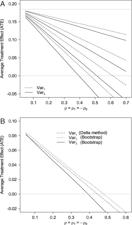
(A) Estimates of the effect of CD4 testing reminder on CD4 test ordering under different combinations of ρ = ρ₁= −ρ₀ and τ. Dashed lines are the estimates of the average treatment effect (ATE) based on Var_τ(S^*|S) (Eq. 11) and solid lines are the estimates of the ATE based on Var_λ(S^*|S) (Eq. 12). The four dashed lines correspond to (from top to bottom) τ = 0.1, 0.2, 0.3, and 0.4. The four solid lines correspond to (from top to bottom) λ(0.1) = 0.0063, λ(0.2) = 0.0245, λ(0.3) = 0.0526, and λ(0.4) = 0.0881. The horizontal gray line on the top is the estimated ATE assuming no uncontrolled confounding. (B) The lower limit of the one-sided 90% confidence interval of the intervention effect for τ = 0.2 for different values of ρ = ρ₁= −ρ₀.

3.2 Cost of abciximab in reducing mortality

Kereiakes et al. (2000) conducted an observational study at the Christ Hospital, Cincinnati, to evaluate the impact of adjunctive pharmacotherapy with abciximab platelet glycoprotein IIb/IIIa blockade administered during percutaneous coronary intervention (PCI) on costs and clinical outcomes in a high-volume interventional practice. It was shown that patients receiving abciximab (treated) had lower mortality rates than those who did not (control) and there was no significant difference in cost. We will focus on the outcome of cost to illustrate how our method can be used to analyze a continuous outcome.

We first did a logarithm-transformation of the cost variable, and then scaled the transformed variable to the unit interval. There are a total of 996 patients, among whom 698 received abciximab and 298 did not. A two-sample T-test shows that the intervention group had significantly higher cost than the control group (0.792 versus 0.777, T-test p<0.0001, two-sided). To account for potential confounders, we fit a probit propensity score model that includes coronary stent deployment (Yes/No), acute myocardial infarction within seven days prior to PCI (Yes/No), diagnosis of diabetes mellitus (Yes/No), and the left ventricular ejection fraction (continuous). These factors univariately correlate with at least one of the two measures: cost or abciximab usage. The inverse propensity score weighting leads to an estimate of the treatment effect of 0.024 (Z-test p<0.0001, two-sided), suggesting again an increase in cost in the intervention group after adjustment.

To investigate potential uncontrolled confounding, we conducted a similar sensitivity analysis. Since the outcome is continuous, the sensitivity analysis will generate estimates of the lower and upper bounds. For this example, it was the lower bound of the causal effect that is of our interest as a positive treatment effect was found. The result is shown in Fig. 3. Clearly, the positive intervention effect is much more sensitive to uncontrolled confounding compared with the previous example. For the estimate of the lower bound of the intervention effect to go below 0, ρ only needs to be a bit over 0.1 when τ = 0.4 or both Var_τ(S^*|S)- and Var_λ(S^*|S)-based analyses. Similarly, or τ = 0.2, the estimate of the lower bound of the intervention effect goes below 0 when ρ>0.25 regardless of the method used. The lower limit of the 90% confidence interval (one-sided) of the lower bound for τ = 0.3 (Fig. 3(B)) shows that as ρ>0.11 the confidence intervals will contain 0. Hence, the sensitivity analysis suggests that the significant intervention effect could have been induced by mild confounding. If we fix λ₁ at 0.0063, 0.0245, 0.0526, and 0.0881, the compatible regions of λ₀ are (0.0001,0.32), (0.0009,0.48), (0.003,0.57), and (0.005,0.64). Therefore, the common values are legitimate.

Figure 3.

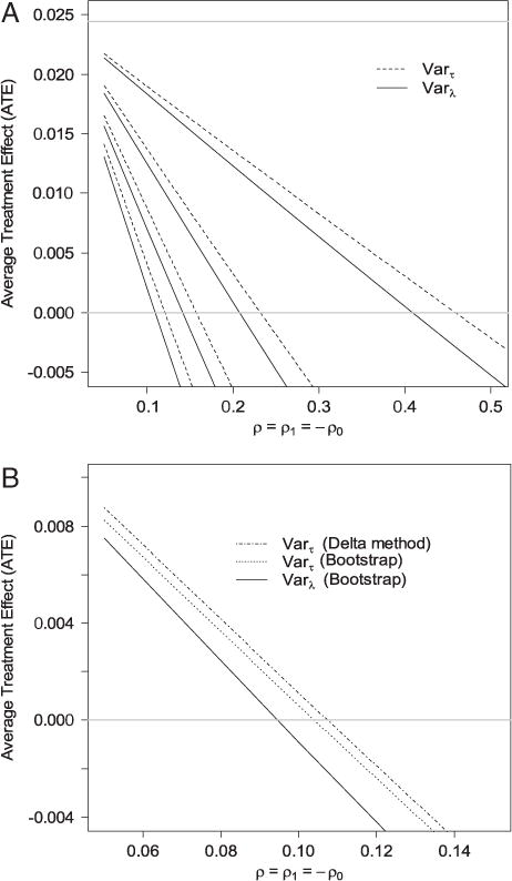
(A) Estimates of the lower bound of the effect of abciximab on cost under different combinations of ρ = ρ₁=−ρ₀ and τ. Dashed lines are the estimates of the ATE based on Var_τ(S^*|S) (Eq. 11) and solid lines are the ATE based on Var_λ(S^*|S) (Eq. 12). The four dashed lines correspond to (from top to bottom) τ = 0.1, 0.2, 0.3, and 0.4. The four solid lines correspond to (from top to bottom) λ(0.1) = 0.0063, λ(0.2) = 0.0245, λ(0.3) = 0.0526, and λ(0.4)= 0.0881. The horizontal gray line on the top is the estimated ATE assuming no uncontrolled confounding. (B) The lower limit of the one-sided 90% confidence interval of the lower bound of the intervention effect for τ = 0.3 for different values of ρ = ρ₁=− ρ₀.

In fact, we intentionally ignored a covariate in our probit model for the pseudo-propensity score: the number of vessels involved in the patient’s initial PCI. Univariate analysis shows that this variable is correlated with both treatment assignment and the cost. When included in the probit model after normalization, $\widehat{\text{τ}}=0.29$ (Wald test P<0.0001, two-sided). Therefore, this variable may be a potential confounder that induces the “treatment effect”. The sensitivity analysis shows that when τ = 0.3 a weak correlation ρ₁= − ρ₀>0.11 could be responsible for the “significant” increase in cost. In fact, when we use the propensity score obtained from the revised probit model with the number of vessels added, the intervention effect is not significant (−0.0019, Z-test p= 0.91, two-sided).

4 Discussion

We propose a general framework and a parametric model for sensitivity analysis built on IPW, which can be used to examine the potential impact of uncontrolled confounding for causal inference using non-randomized data. It should be noted that the method can be readily applied to inference of marginal means when the data are subject to non-ignorable missingness (Little and Rubin, 1987). Our method offers a simple, intuitively appealing, and easy-to-implement procedure, which is only based on two parameters: the variance of the multiplicative error of the propensity score and its correlation with a potential outcome. Although we only illustrate the proposed methods through the estimation of ATE, the method can be readily applied to ATE on the treated (ATT). To see this, note that

$$E\left(Y_1-Y_0|Z=1\right)=E\left(Y_1|Z=1\right)-\frac{E\left(Y_0\right)-Pr\left[Z=0\right]E\left(Y_0|Z=0\right)}{Pr\left[z=1\right]}$$

Since Pr[Z= 1], E(Y₀|Z = 0), and E(Y₁|Z = 1) are estimable, the bounds of E(Y₀) can be directly translated to those of E(Y₁−Y₀|Z= 1).

We focus on uncontrolled confounding and its impact on causal inference in this article. Therefore, our working assumption is that the pseudo-propensity score model for included confounders is correctly specified. Our method does not address the bias induced by model-misspecification. This is why we considered the probit model instead of the logit model in Section 2.3. The reason is that if the true propensity score is a probit model, then the pseudo-propensity score is still a probit model, which eliminates model-misspecification in the pseudo-propensity score. This leaves uncontrolled confounders the only source of bias. It is well known that the logit model does not have this kind of property. Nevertheless, our general framework allows one to use any method to fit the pseudo-propensity score including the logit model. The probit model simply serves as a tool to guide the parameter specifications. In reality, bias can be induced by both model-misspecification and uncontrolled confounding. Therefore, an appropriate procedure should be employed to examine both factors for the evaluation of the robustness of the conclusion.

Sensitivity analysis is a critical component in observational studies to examine the robustness of the conclusion. For practical purposes, a key to construct such analysis is simple and sensible parameters, the scales of which are familiar to investigators. We choose to base our sensitivity analysis on (ρ,τ) as these two measures are of broad familiarity with clear and sensible scales. A sensitivity analysis should account for confounders we are not aware of. By its definition, the associations of these confounders with treatment assignment and potential outcomes are hard to postulate based on empirical experience/data. Therefore, the solution is to examine the impact of confounding under a range of different levels of these associations (i.e. low and high).

The motivation to restrict a continuous variable to the [0,1] interval is to bound its variance (from both up and below) by estimable parameters and the non-estimable target (i.e. E(Y₁), see Eq. 6). Then in Eq. (3), one can replace Var(Y₁) with its upper and lower bounds. This automatically eliminates Var(Y₁) from the equation so that the users do not need to worry about specifying Var(Y₁) (non-estimable when there is uncontrolled confounding) and its effect on the bias. Moreover, our strategy avoids the difficulty in having incompatible mean and variance values for families of distributions where the two parameters are related. Although general statistical theories often apply to continuous variables taking values on the whole real line, most of the continuous measures in real life problems are finite in nature. A simple method would be to scale the measure to the [0,1] interval by using reasonable lower and upper bounds. In our opinion, this is a practically very feasible solution. To be conservative, one can also choose relatively extreme bounds. Even without assumptions of the upper and lower bounds, one can still use monotone non-linear transformations (i.e. probit and inverse logit functions) to rescale the original variable to [0,1]. The bounds of the mean of the potential outcome in the original scale can be obtained by the Taylor expansion followed by plugging in the bounds of the mean and the variance of the transformed scale. For instance, if O is the original scale and Y is the transformed scale with O = f(Y), then

$$E\left(O_1\right)=E\left[f\left(Y_1\right)\right]\approx f\left(E\left(Y_1\right)\right)+\frac{1}{2}\frac{d^{2}f}{2d{Y}_1^2}{|}_{E\left(Y_1\right)}\ast \text{Var}\left(Y_1\right)\text{.}$$

Based on the shape of the second derivative of f in the interval defined by the bounds of E(Y₁), one can plug in the relevant bounds for E(Y₁) and Var(Y₁) to obtain bounds for E(O₁).

From the analytical standpoint, in many cases sensitivity analysis will generate some bounds. These bounds add another level of uncertainty in addition to sampling variation. Therefore, for a sensitivity analysis to be useful and informative, these bounds should be as sharp as possible to accurately characterize the robustness. Although we consider compatibility of λ₁ and λ₀ in our analysis, the compatibility between λ₁ and ρ₁ (or between λ₀ and ρ₀) is more complicated and is not studied in this article. Therefore, our bounds are likely not to be sharp. Nevertheless, we believe our method is a balance of simplicity/sensibility and sharpness to be useful and accessible to medical researchers and scientists. A future direction is to investigate the simplification of the compatibility between λ₁ and ρ₁ to improve the sharpness of the bounds.

Appendix A

A.1 Proof of Result 1

$$\begin{array}{c}{\text{ν}}_0={\text{Var(}\epsilon }_0\text{)}\\ =\text{Var}\left[\frac{1-S^{\ast }}{1-S}\right]\\ =E\left[\frac{{\text{Var(S}}^{\ast }|S\text{)}}{{(1-S)}^2}\right](\text{since }E{\text{(S}}^{\ast }|S\text{)}=S)\end{array}$$

$\text{Let }g(S)={\text{Var(S}}^{\ast }|S\text{)},0\le g\le S(1-S)$

$$\begin{array}{c}{v}_0=E\left[\frac{g}{{(1-S)}^2}\right]\\ =E\left[\frac{I(S\ge q_2)g}{{(1-S)}^2}\right]+E\left[\frac{I(S<q_2)g{S}^2}{S^2{(1-S)}^2}\right]\\ \le E\left[\frac{I(S\ge q_2)g}{{(1-S)}^2}\right]+E\frac{q_2^2}{{(1-q_2)}^2}E\left[\frac{I(S<q_2)g}{S^2}\right]\\ =E\left[\frac{I(S\ge q_2)S}{1-S}\right]+E\left[\frac{I(S\ge q_2)(g-S(1-S))}{{(1-S)}^2}\right]+\frac{q_2^2}{{(1-q_2)}^2}E\left[\frac{I(S<q_2)g}{S^2}\right]\\ \le \left[\frac{I(S\ge q_2)S}{1-S}\right]+\frac{q_2^2}{{(1-q_2)}^2}\left\{E\left[\frac{I(S\ge q_2)g}{S^2}\right]-E\left[\frac{I(S\ge q_2)(1-S)}{S}\right]\right\}+\frac{q_2^2}{{(1-q_2)}^2}\left[\frac{I(S<q_2)g}{S^2}\right]\\ =E\left[\frac{I(S\ge q_2)S}{1-S}\right]+\frac{q_2^2}{{(1-q_2)}^2}\left[E\left(\frac{g}{S^2}\right)-E\left(\frac{I(S\ge q_2)(1-S)}{S}\right)\right]\\ =E\left[\frac{I(S\ge q_2)S}{1-S}\right](E(g/S^2)=E[I(S\ge q_2)S/(1-S)]=v_1\text{ by the definition of g and }{q}_2).\end{array}$$

Therefore, λ₀ = ν₀/V₀≤ E[I(S≥q₂)S/(1−S)]/V₀. Analogously, it can be shown that λ₀≥E[I(S≤q₁)S/(1−S)]/V₀.

A.2 Derivation of Var_τ(S^*|S)

$$\begin{array}{l}{E}_{\text{τ}}(S{\ast }^2|S)={{\displaystyle \int }}_{-\infty }^{\infty }{\mathrm{\Phi }}^2(W+\text{τ}u)\varphi (u)du={{\displaystyle \int }}_{-\infty }^{\infty }\left({{\displaystyle \int }}_{-\infty }^{W+\text{τ}u}\varphi (t)dt\right)\left({{\displaystyle \int }}_{-\infty }^{W+\text{τ}u}\varphi (v)dv\right)\varphi \left(u\right)du\hfill \\ =\text{Pr}\left(T-\text{τ}U\le W\&V-\text{τ}U\le W\right)\left(T,V,\text{and }U\text{ are independent standard normal variables}\right)\hfill \\ =\text{ Pr}\left(T_1\le \text{W}\&T_2\le W\right)\left(T_1,T_2~N\left(0,1+{\text{τ}}^2\right),\text{ Cov}\left(T_{1,}{T}_2\right)={\text{τ}}^2\right)\hfill \\ =F_{\text{τ}}\left(W,W\right)\left(F_{\text{τ}}\text{ is the cumulative distribution function of the joint distribution of }{T}_1\text{ and }{T}_2\right)\hfill \\ F_{\text{τ}}(\sqrt{1+{\text{τ}}^2}{\text{Φ}}^{-1}\left(S\right),\sqrt{1+{\text{τ}}^2}{\mathrm{\Phi }}^{-1}(S))(\mathrm{because}S=\mathrm{\Phi }(W/\sqrt{1+{\text{τ}}^2})).\hfill \end{array}$$

Therefore; ${\text{Var}}_{\mathrm{\tau }}\left(S^{\ast }|S\right)=F_{\text{τ}}\left(\sqrt{1+{\text{τ}}^2}{\mathrm{\Phi }}^{-1}\left(S\right),\sqrt{1+{\text{τ}}^2}{\mathrm{\Phi }}^{-1}\left(S\right)\right)-S^2$

A.3 Asymptotic distribution of bound estimators based on the probit model

Here, we show the derivation of the asymptotic distributions of ${\widehat{l}}_1$ and ${\widehat{L}}_1$. Similar reasoning can be applied to derive the asymptotic distributions of ${\widehat{l}}_1$ and ${\widehat{L}}_1$ and the estimates of the bounds for the causal effect. We will consider a continuous outcome.

Let (X_i, Z_i, Y_i) (i = 1,2,…,n) be the observed data for unit i. Under the probit parametric model, $S_i=\text{Pr}(Z_i=1|{\text{X}}_i)=\mathrm{\Phi }(W({\text{X}}_i)/\sqrt{1+{\text{τ}}^2)}=S_i({\text{X}}_i,\text{β}),$ where W is a function of X_i that also depends on a vector of parameters β. Let G_i = Y_iZ_i/S_i and $H_i=F_{\text{τ}}(\sqrt{1+{\text{τ}}^2}{\mathrm{\Phi }}^{-1}(S_i),\sqrt{1+{\text{τ}}^2}{\text{Φ}}^{-1}(S_i))/S_i^2-1.$. Therefore, E(G_i) = θ₁ and E(H_i) = v₁. Denote ζ = (θ₁,π, ϕ₁ = E(YZ), δ₁ = E(Y²Z),v₁)^T and ${\text{O}}_i={(G_i+{\text{γ}}_{\text{G}}^{\text{T}}{\text{IF}}_i,Z_i,Y_i{Z}_i,Y_i^2{Z}_i,H_i+{\text{γ}}_{\text{G}}^{\text{T}}{\text{IF}}_i)}^{\text{T}},$, where IF_i is the influence function for β under the parametric probit model; ${\text{γ}}_{\text{G}}=E(\partial G/\partial \beta );{\text{γ}}_{\text{H}}=E(\partial H/\partial \beta \text{)}\text{.}$ It is straightforward to show by the fact E(IF_i) = 0 and central limit theorem that under suitable regularity conditions

$$\frac{1}{\sqrt{n}}\sum _{i=1}^n({\text{O}}_i-\mathbf{\zeta })\stackrel{D}{\to }N\left(0,\mathbf{\Lambda }\right),$$

where Λ is the variance-covariance matrix of O_i.

Since ${\text{μ}}_1={\mathrm{\phi }}_1/\text{π}$ and η₁ = δ₁/π, the bounds determined by (6) are functions of ζ: l₁ = l₁(ζ) and L₁ = L₁(ζ). Then a direct application of the delta method leads to the asymptotic distributions of ${\widehat{l}}_1$ and ${\widehat{L}}_1$.

References

- Arah OA, Chiba Y, Greenland S. Bias formulas for external adjustment and sensitivity analysis of unmeasured confounders. Annals of Epidemiology. 2008;18:637–646. doi: 10.1016/j.annepidem.2008.04.003. [DOI] [PubMed] [Google Scholar]
- Bang H, Robins JM. Doubly robust estimation in missing data and causal inference models. Biometrics. 2005;61:962–973. doi: 10.1111/j.1541-0420.2005.00377.x. [DOI] [PubMed] [Google Scholar]
- Brumback BA, Hernan MA, Haneuse SJ, Robins JM. Sensitivity analyses for unmeasured confounding assuming a marginal structural model for repeated measures. Statistics in Medicine. 2004;23:749–767. doi: 10.1002/sim.1657. [DOI] [PubMed] [Google Scholar]
- Cochran WG. Matching in analytical studies. American Journal of Public Health and the Nations Health. 1953;43:684–691. doi: 10.2105/ajph.43.6_pt_1.684. [DOI] [PMC free article] [PubMed] [Google Scholar]
- Cole SR, Hernan MA, Margolick JB, Cohen MH, Robins JM. Marginal structural models for estimating the effect of highly active antiretroviral therapy initiation on CD4 cell count. American Journal of Epidemiology. 2005;162:471–478. doi: 10.1093/aje/kwi216. [DOI] [PubMed] [Google Scholar]
- Copas JB, Li HG. Inference for non-random samples. Journal of the Royal Statistical Society, Series B. 1997;59:55–95. [Google Scholar]
- Greenland S. Multiple-bias modelling for analysis of observational data (with discussion) Journal of the Royal Statistical Society, Series A. 2005;168:267–306. [Google Scholar]
- Hernan MA, Robins JM. Method for conducting sensitivity analysis. Biometrics. 1999;55:1316–1317. [PubMed] [Google Scholar]
- Hirano K, Imbens GW. Estimation of causal effects using propensity score weighting: an application to data on right heart catheterization. Health Services and Outcomes Research Methodology. 2001;2:259–278. [Google Scholar]
- Holland PW. Statistics and causal inference. Journal of the American Statistical Association. 1986;81:945–960. [Google Scholar]
- Imbens GW. Sensitivity to exogeneity assumptions in program evaluation. American Economic Review. 2003;93:126–132. [Google Scholar]
- Kereiakes DJ, Obenchain RL, Barber BL, Smith A, McDonald M, Broderick TM, Runyon JP, Shimshak TM, Schneider JF, Hattemer CR, Roth EM, Whang DD, Cocks D, Abbottsmith CW. Abciximab provides cost-effective survival advantage in high-volume inter-ventional practice. American Heart Journal. 2000;140:603–610. doi: 10.1067/mhj.2000.109647. [DOI] [PubMed] [Google Scholar]
- Ko H, Hogan JW, Mayer KH. Estimating causal treatment effects from longitudinal HIV natural history studies using marginal structural models. Biometrics. 2003;59:152–162. doi: 10.1111/1541-0420.00018. [DOI] [PubMed] [Google Scholar]
- Kuroki M, Cai Z. Formulating tightest bounds on causal effects in studies with unmeasured confounders. Statistics in Medicine. 2008;27:6597–6611. doi: 10.1002/sim.3430. [DOI] [PubMed] [Google Scholar]
- Lin DY, Psaty BM, Kronmal RA. Assessing the sensitivity of regression results to unmeasured confounders in observational studies. Biometrics. 1998;54:948–963. [PubMed] [Google Scholar]
- Little RJA, Rubin DB. Statistical Analysis with Missing Data. Wiley; New York: 1987. [Google Scholar]
- MacLehose RF, Kaufman S, Kaufman JS, Poole C. Bounding causal effects under uncontrolled confounding using counterfactuals. Epidemiology. 2005;16:548–555. doi: 10.1097/01.ede.0000166500.23446.53. [DOI] [PubMed] [Google Scholar]
- Robins JM. Association, causation, and marginal structural models. Synthese. 1999;121:151–179. [Google Scholar]
- Robins JM, Rotnitzky A, Zhao L. Estimation of regression coefficients when some regressors are not always observed. Journal of the American Statistical Association. 1994;89:846–866. [Google Scholar]
- Rosenbaum PR. Observational Studies. Springer; New York: 1995. [Google Scholar]
- Rosenbaum PR, Rubin DB. Assessing sensitivity to an unobserved binary covariate in an observational study with binary outcome. Journal of the Royal Statistical Society, Series B. 1983a;45:212–218. [Google Scholar]
- Rosenbaum PR, Rubin DB. The central role of the propensity score in observational studies for causal effects. Biometrika. 1983b;70:41–55. [Google Scholar]
- Rosenbaum PR, Rubin DB. The bias due to incomplete matching. Biometrics. 1985;41:103–116. [PubMed] [Google Scholar]
- Rubin DB. Matching to remove bias in observational studies. Biometrics. 1973;29:159–183. [Google Scholar]
- Rubin DB. Estimating causal effects of treatments in randomized and nonrandomized studies. Journal of Educational Psychology. 1974;66:688–701. [Google Scholar]
- Rubin DB. Bayesian inference for causal effects: the role of randomization. Annals of Statistics. 1978;6:34–58. [Google Scholar]
- Rubin DB. Causal inference using potential outcomes: design, modeling, decisions. Journal of the American Statistical Association. 2005;100:322–331. [Google Scholar]
- Rubin DB, Thomas N. Matching using estimated propensity scores: relating theory to practice. Biometrics. 1996;52:249–264. [PubMed] [Google Scholar]
- Sturmer T, Schneeweiss S, Rothman KJ, Avorn J, Glynn RJ. Performance of propensity score calibration – a simulation study. American Journal of Epidemiology. 2007a;165:1110–1118. doi: 10.1093/aje/kwm074. [DOI] [PMC free article] [PubMed] [Google Scholar]
- Sturmer T, Schneeweiss S, Rothman KJ, Avorn J, Glynn RJ. Propensity score calibration and its alternatives. American Journal of Epidemiology. 2007b;165:1122–1123. doi: 10.1093/aje/kwm068. [DOI] [PMC free article] [PubMed] [Google Scholar]
- Vander Weele TJ. The sign of the bias of unmeasured confounding. Biometrics. 2008;64:702–706. doi: 10.1111/j.1541-0420.2007.00957.x. [DOI] [PubMed] [Google Scholar]
- Were MC, Shen C, Tierney WM, Mamlin JJ, Biondich PG, Li X, Kimaiyo S, Mamlin BW. Evaluation of computer-generated reminders to improve CD4 laboratory monitoring in sub-Saharan Africa: a prospective comparative study. Journal of the American Medical Informatics Association. 2011;18:150–155. doi: 10.1136/jamia.2010.005520. [DOI] [PMC free article] [PubMed] [Google Scholar]
Associated Data
This section collects any data citations, data availability statements, or supplementary materials included in this article.