Multiparametric brainstem segmentation using a modified multivariate mixture of Gaussians

Abstract

The human brainstem is a densely packed, complex but highly organised structure. It not only serves as a conduit for long projecting axons conveying motor and sensory information, but also is the location of multiple primary nuclei that control or modulate a vast array of functions, including homeostasis, consciousness, locomotion, and reflexive and emotive behaviours. Despite its importance, both in understanding normal brain function as well as neurodegenerative processes, it remains a sparsely studied structure in the neuroimaging literature. In part, this is due to the difficulties in imaging the internal architecture of the brainstem in vivo in a reliable and repeatable fashion.

A modified multivariate mixture of Gaussians (mmMoG) was applied to the problem of multichannel tissue segmentation. By using quantitative magnetisation transfer and proton density maps acquired at 3 T with 0.8 mm isotropic resolution, tissue probability maps for four distinct tissue classes within the human brainstem were created. These were compared against an ex vivo fixated human brain, imaged at 0.5 mm, with excellent anatomical correspondence. These probability maps were used within SPM8 to create accurate individual subject segmentations, which were then used for further quantitative analysis. As an example, brainstem asymmetries were assessed across 34 right-handed individuals using voxel based morphometry (VBM) and tensor based morphometry (TBM), demonstrating highly significant differences within localised regions that corresponded to motor and vocalisation networks. This method may have important implications for future research into MRI biomarkers of pre-clinical neurodegenerative diseases such as Parkinson's disease.

Highlights

• •We developed a method to allow automated segmentation of the brainstem in vivo at 3 T.
• •The internal structure of the brainstem can be partitioned into four tissue types.
• •Good anatomical correspondence with ex vivo MR brainstem anatomy is demonstrated.
• •The brainstems of 34 subjects are segmented, and quantitatively analysed.
• •Significant brainstem asymmetries are demonstrated in vivo.

1. Introduction

The human brainstem is a complex but highly organised structure, densely packed with long projecting axons and interspersed nuclei. It not only serves as a conduit for motor and sensory information, but also is the location of multiple primary nuclei that control or modulate a vast array of vital functions including homeostasis, consciousness, locomotion, and reflexive and emotive behaviours (Parvizi and Damasio, 2001). There is increasing evidence that several neurodegenerative diseases, such as Parkinson's disease (Del Tredici et al., 2002; Hawkes et al., 2010) and Alzheimer's disease (Grinberg et al., 2009; Simic et al., 2009), are characterised by early involvement of this region during long prodromal periods, many years before overt clinical symptoms are detectable. Despite its importance, both in understanding normal brain function as well as neurodegenerative processes, it remains a relatively sparsely studied structure in the neuroimaging literature. In part, this is due to the difficulties in resolving the internal architecture of the brainstem in vivo in a reliable and repeatable fashion. In this paper, we use high-resolution quantitative imaging to obtain accurate measurements within the human brainstem, and utilise these to develop a tissue segmentation algorithm that allows an automated, unbiased approach to quantitative analysis within this region.

Mutichannel tissue segmentation is a method that can potentially improve the segmentation accuracy of cortical tissue types (Ortendahl and Hylton, 1986). It is known that different midbrain structures can be better visualised using specific MRI contrast, for example proton density imaging for the pedunculopontine nucleus (Zrinzo et al., 2008) or magnetisation transfer (MT) imaging for the substantia nigra (Helms et al., 2009). By exploiting the information from several different imaging contrasts using multivariate data-clustering techniques, a more parsimonious segmentation of structures can be achieved, where a single channel fails. The mixture of Gaussians model (MoG) is a well-established technique in data clustering (Hasselblad, 1966; see Bishop, 2006 for examples), and has been extensively used in tissue segmentation algorithms (eg. Ashburner and Friston, 2005). Here we modify the standard multivariate MoG algorithm to iteratively estimate and refine spatial tissue probability maps from multispectral data. The modified multivariate mixture of Gaussians (mmMoG) was then optimised specifically for brainstem segmentation using high-resolution quantitative data, and used to generate four unique tissue probability maps (TPMs). Quantitative MRI yields accurate and reproducible MR measurements that meaningfully reflect underlying biological properties within the various tissues (Tofts, 2003). It is these properties that are exploited to classify and segment homologous tissue types using a population of subjects.

The primary aim of this study was to develop a method to segment the internal structures within the human brainstem using quantitative imaging. Thus, we aimed to improve the sensitivity of pre-existing neuroimaging analysis techniques such as voxel based morphometry (VBM) (Ashburner and Friston, 2000) within this region. To test the brainstem specific segmentation algorithm we assessed human brainstem asymmetries across 34-right handed subjects using tensor based morphometry (TBM) and VBM.

2. Methods

2.1. Subjects

Thirty-four healthy right-handed adults (seventeen males, mean age for males = 31.1 y, for females = 22.6 y), underwent a single MRI scanning session at the Wellcome Trust Centre for Neuroimaging. Involvement of human volunteers was approved by the local ethics committee, and each subject provided written informed consent prior to MRI examination.

In vivo results were validated against a brain specimen of a 57 year-old male, who died of a cardiac arrest. Autopsy was performed approximately 16 h post mortem for unrelated diagnostic purposes at the Göttingen University Medical Centre, Germany. Informed written consent had been obtained from the subjects next of kin prior to autopsy, as approved by the local ethics committee. The brain was fixated in phosphate-buffered saline with 3.7% formaldehyde for three weeks eventually diagnosed as macroscopically normal.

2.2. In vivo image acquisition

All examinations were performed on a 3 T whole-body MRI system (Magnetom TiM Trio, Siemens Healthcare, Erlangen). 3D multi-echo FLASH images were acquired at 0.8 mm isotropic resolution with MT, T1 and proton density (PD)-weighted contrast following the multi-parameter quantitative mapping protocol described in (Helms et al., 2008). To improve SNR, a 32-channel receive head coil was used and the protocol was repeated twice to allow the images to be averaged. The total acquisition time was 1 h and 15 min. Full imaging parameters are summarised in Table 1. For each subject quantitative MT, R1 (= 1/T1), PD and R2* (equal to 1/T2*) maps were extracted from the acquired images using in-house MATLAB code. In addition, B1-field maps (4 mm isotropic resolution) were acquired using a 3D EPI SE/STE method (Lutti et al., 2010, 2012) and used to correct the R1 maps for RF transmit field inhomogeneity effects. The systematic bias of the PD maps by the inhomogeneous sensitivity profile of the receive head coil was corrected using the UNICORT algorithm (Weiskopf et al., 2011). Quantitative PD estimates were obtained by scaling the corrected PD maps by the expected average proton density of white matter (69% (Tofts, 2003)).

Table 1.

Imaging parameters.

Image type	Slice no.	FOV (mm2)	Acquisition matrix (voxels)	TR (ms)	TE (ms)	Flip angle	Echo no.	Notes
MT	240	216 × 256	270 × 320	23.7	[2.2:2.55:9.85]	6	4	Parallel imaging (GRAPPA) along phase encoding direction Partition partial Fourier (6/8) Bandwidth = 425 Hz/pixel
T1	240	216 × 256	270 × 320	23.7	[2.2:2.55:9.85]	28	4
PD	240	216 × 256	270 × 320	23.7	[2.2:2.55:9.85]	6	4
B1-map	48	192 × 256	48 × 64	500	(SE:39.38; STE:70.58)	SE:[270: − 10:130]	2
Fieldmap	64	192 × 192	64 × 64	1020	10; 12.46	90;	2

2.3. Post mortem image acquisition

The fixated brain specimen was sealed in double plastic bags and scanned on an identical MRI system at the Göttingen University Medical Centre, Germany, using the quadrature birdcage knee coil. Care was taken to minimise air pockets and to prevent folding artefacts from overlapping with brain. Non-selective 3D FLASH MRI (256 axial partitions of 384 × 384 pixels at 0.5 mm isotropic resolution) with off-resonance MT pre-saturation (at + 1.2 kHz, 9.984 ms Gaussian, 500°) was performed. Eight gradient echoes at echo times of 2.46, 4.92, and 19.68 ms (500 Hz/pixel) were averaged to increase SNR (Helms et al., 2009), yielding a combination of PD, MT and moderate T2* weighting. At a repetition time of 39 ms, a flip angle of 16° was chosen to increase SNR and suppress the fluid signal (Helms et al., 2011). Total measurement time was 140 min for four averages.

2.4. Pre-processing

A brainstem mask for each individual was created from the MT maps using ITK-SNAP (Yushkevich et al., 2006). This was mainly done using the “snake” function to automatically segment the brainstem region based on intensity, but the superior and inferior boundaries required manual demarcation. The following anatomical landmarks were used: Inferiorly, the level of the foramen magnum; posteriorly, a vertical line following the most posterior aspect of the medulla, which included part of the middle and superior cerebellar peduncles. Superiorly, the boundary of the cerebral aqueduct and 3rd ventricle was used. At this level, the lateral margins of the brainstem mask were demarcated by the lateral border of the cerebral peduncle, the superior colliculi and medial geniculate nuclei posteriorly, and the posterior edge of the mammilo-thalamic tract anteriorly. Additionally any cerebellar grey matter was excluded. These boundaries were chosen to allow the masking procedure to be consistent across subjects whilst including all of the midbrain and brainstem in the segmentation step. The accuracy of the masking procedure was assessed by examining the group-averaged brainstem mask after warping. For the purpose of co-registration, the MT maps were initially segmented into grey, white and CSF tissue classes at the native resolution (0.8 mm) using the unified segmentation withinSPM8 (http://www.fil.ion.ucl.ac.uk/spm/) (Ashburner and Friston, 2005). These segmentations were registered to a common group-average 0.8 mm isotropic template using a diffeomorphic registration algorithm (Ashburner and Friston, 2011). Then, the individual MT and PD maps were all warped to the common template space, along with the individual brainstem masks. These masks were averaged, smoothed by a Gaussian kernel of 1 mm full-width-at-half-maximum (FWHM) and binarised to create a common brainstem region. This was to refine the segmentation step (outlined below) by ensuring that all subjects were included in the estimation of the TPMs across the brainstem region.

2.5. Multichannel segmentation of quantitative images

Quantitative mapping yields MR parameter estimates that are highly consistent across subjects for homologous tissue types across subjects, which normally cannot be achieved using conventional MR imaging (Draganski et al., 2011). Therefore, quantitative MRI data (so called “maps”) allow information to be shared across a population of subjects. This should yield a more parsimonious model than if the subjects' data were segmented individually. Here, we describe a segmentation approach for partitioning spatially normalised quantitative images from a population of subjects, into K different tissue probability maps. It is the generation of these probability maps from populations of quantitative multivariate data that distinguishes this approach from classical unified segmentation (Ashburner and Friston, 2005). To define the approach: Each spatially normalised image contains J voxels, such that the intensity of the jth voxel of the ith subject may be represented by x_ij. If the data is multi-spectral (i.e., consists of quantitative maps of multiple parameters such as PD and MT maps) the intensity at voxel j of subject i will be a vector of M values, where M is the number of quantitative maps per subject.

The objective of this clustering may be viewed as factorising the data into the K tissue probability maps (TPMs) of interest, and K representations of the probability density functions of the intensities of the tissue types. The kth tissue type of the jth voxel of the TPM is denoted by b_kj, such that b_kj ≥ 0 and ∑ _k = 1^K b_kj = 1. In the current model, the intensities within each of the tissue classes are assumed to be drawn from a multivariate normal distribution, such that x ~$\mathcal{N}$(μ_k,S_k), which reflects the number of distinctive quantitative maps utilised. Determining a maximum likelihood estimate for this factorisation involves maximising the following log-likelihood objective function.

$$\mathcal{E}={\displaystyle \sum }_{i=1}^I{\displaystyle \sum }_{j=1}^{J}log\left({\displaystyle \sum }_{k=1}^K{b}_{\mathit{kj}}p\left(x_{\mathit{ij}}|{\mu }_k,S_k\right)\right)\text{.}$$ (1)

Initially, class memberships of voxels from the various subjects are assumed to be unknown. Optimising this objective function involves introducing hidden variables, z_ijk, which encode these class memberships. This leads to the following expectation–maximisation algorithm for optimising the model. To avoid bias, randomised starting estimates for the parameters were used. The following steps are repeated for each slice until the log-likelihood no longer increases.

• 1.
  E-step. Estimate the hidden variables for the current iteration (n), using the parameter estimates from the previous iteration (n − 1).

  $$z_{\mathit{ijk}}^{\left(n\right)}=\frac{b_{\mathit{kj}}^{\left(n-1\right)}p\left(x_{\mathit{ij}}|{\mu }_k^{\left(n-1\right)},S_k^{\left(n-1\right)}\right)}{{{\displaystyle \sum }}_{l=1}^K{b}_{\mathit{lj}}^{\left(n-1\right)}p\left(x_{\mathit{ij}}|{\mu }_l^{\left(n-1\right)},S_l^{\left(n-1\right)}\right)}\text{.}$$ (2)
  This requires the probability density of an M-dimensional multivariate Gaussian, which is:

  $$p\left(x_{\mathit{ij}}|{\mu }_k,S_k\right)=\frac{1}{\sqrt{{\left(2\pi \right)}^{M}det\left|S_k\right|}}exp\left(-\frac{1}{2}\left(x_{\mathit{ij}}-{\mu }_k\right)S_k^{-1}\left(x_{\mathit{ij}}-{\mu }_k\right)\right)\text{.}$$ (3)

  Specifically, in this current example a bivariate Gaussian was used to model the intensity distributions from the MT and PD maps.

• 2.
  M-step. Then use the current estimates of the hidden variables to determine the parameter estimates that maximise the objective function. The tissue probability maps are updated by:

  $$b_{\mathit{kj}}^{\left(n\right)}=\frac{{{\displaystyle \sum }}_{i=1}^I{z}_{\mathit{ijk}}^{\left(n\right)}}{{{\displaystyle \sum }}_{i=1}^I{{\displaystyle \sum }}_{l=1}^K{z}_{\mathit{ijk}}^{\left(n\right)}}\text{.}$$ (4)
  Means and variances of the intensity distributions are re-estimated by:

  $${\mu }_k^{\left(n\right)}=\frac{{{\displaystyle \sum }}_{i=1}^I{{\displaystyle \sum }}_{j=1}^J{z}_{\mathit{ijk}}^{\left(n\right)}{x}_{\mathit{ij}}}{{{\displaystyle \sum }}_{i=1}^I{{\displaystyle \sum }}_{j=1}^J{z}_{\mathit{ijk}}^{\left(n\right)}}$$ (5)

  $$S_k^{\left(n\right)}=\frac{{{\displaystyle \sum }}_{i=1}^I{{\displaystyle \sum }}_{j=1}^J{z}_{\mathit{ijk}}^{\left(n\right)}\left(x_{\mathit{ij}}-{\mu }_k^{\left(n\right)}\right){\left(x_{\mathit{ij}}-{\mu }_k^{\left(n\right)}\right)}^T}{{{\displaystyle \sum }}_{i=1}^I{{\displaystyle \sum }}_{j=1}^J{z}_{\mathit{ijk}}^{\left(n\right)}}\text{.}$$ (6)

The algorithm converges to a local (rather than the global) optimum. Therefore, the final solution is dependent on the starting estimates used to initialise the algorithm. For this reason the whole pipeline was repeated several times to ensure that the solutions obtained were stable, and K was varied to produce a range of TPMs which were inspected and the minimum number that produced anatomically congruent, homologous tissue types without over-clustering was selected. Over-clustering was judged to be present when the same tissue type was present in several TPMs, and subsequent intensity plots were highly overlapping. Practically, the optimal number was found at K = 6, generating four brainstem tissues, one containing partial volume edge voxels and one as a non-brainstem class. The latter two were summed into a single map. Once the TPMs were generated and visually inspected, these were then used in SPM8 “New Segment” to produce individual level segmentations as outlined below.

2.6. Visualisation

The probability maps were compared against a fixed specimen imaged at a high-isotropic resolution of 0.5 mm. For illustrative purposes, these images were labelled at six representative slices using the Duvernoy's brainstem atlas as a reference (Naidich and Duvernoy, 2009) and presented in the results. For further anatomical validation, three representative figures of MR microscopy at 9.4 T were taken from Duvernoy's brainstem atlas with permission, and the corresponding TPM projected directly onto these ex-vivo sections. Finally, the three-dimensional structure formed by each tissue class was visualised using SPM8 to render the TPM, binarised at a threshold of 0.5. Subsequent VBM results were also projected on to these surfaces.

2.7. Individual level segmentation

The calculated tissue probability maps (TPMs) were used with SPM8's “New Segment” algorithm. Specifically, five tissue classes were used; four within brainstem and one for everything else. Two Gaussians were used to model each tissue class (Ashburner and Friston, 2005) except for the periaqueductal grey (PAG) matter (one Gaussian) and non-brainstem (eight Gaussians). Individual level segmentations were generated from the MT and PD maps, cropped to include the brainstem region only, which increased the computational speed. All the images from each of the four tissue classes were then left–right flipped and re-sliced to allow brainstem asymmetries to be assessed using VBM as a proof of concept. All of the flipped and un-flipped brainstem tissue classes were re-warped back to a group average using the same diffeomorphic registration algorithm to allow re-estimation of the Jacobians for subsequent TBM and VBM analyses. The deformation fields were then used to warp each tissue class to the common template, and resulting images “modulated” by multiplying with the corresponding Jacobian determinants.

2.8. Brainstem asymmetries

For VBM, a design matrix for a paired t-test between flipped and un-flipped brainstems was constructed for each of the warped and modulated tissue classes, including age, sex and total intracranial volume as covariates in the model. Implicit masking was used with overall grand mean scaling global normalisation. For each tissue class, we examined the contrast showing increased tissue density in the un-flipped as compared to the flipped images. In this, significant results would represent localised brainstem regions with significant asymmetries in a right-handed population. These were corrected for multiple comparisons at a family wise error (FWE) p < 0.05. They were visualised both on an example warped MT image and also on group-averaged renderings of each tissue type. Tensor based morphometry (TBM) is similar to VBM, except that statistical analysis is carried out directly on maps of the Jacobian determinants instead of the warped modulated tissue class maps. Besides the input images, the remaining set-up and analysis was identical.

3. Results

3.1. Tissue probability maps

Six tissue classes were initially generated, but subsequent inspection revealed that one only represented edge of brainstem voxels and so was added to the non-brainstem tissue class. The remaining classes represented brainstem white matter and three grey matter classes: Tissue class one (brainstem grey matter) predominately included structures consistent with monoamine neuron groups including the substantia nigra, ventral tegmental area and raphe nuclei. It also encompassed cranial nerve nuclei and the inferior olivary nucleus. Tissue class two (reticulated grey matter) consisted mainly of the reticular and pontine nuclei, but also included tissue surrounding the inferior olivary nucleus which was most likely the amiculum. Tissue class three was specific for the peri-aqueductal grey (PAG). This region also included some voxels at the edge of the brainstem that, due to partial volume effects at the brainstem-CSF interface, shared similar intensity profiles. However in practical terms, these were masked out from any statistical analysis using a manually refined ROI encapsulating just the PAG and central grey matter, although a threshold of 0.8 also excluded the majority of the non-PAG regions in this class. Tissue class 4 was specific for brainstem white matter. The brainstem tissue classes are summarised in Fig. 1, with comparison against the corresponding labelled sections of the ex vivo high-resolution brainstem. Fig. 2 shows the Gaussian distributions associated with each tissue class; the MPM values have been normalised by the maximum corresponding parameter so both could be visualised on a scale between 0 and 1. It demonstrates that the PAG was a highly unique class with very low MT and high PD intensities, as was the brainstem grey matter with low MT and medium PD values. Tissue classes 4 (white matter) and 2 (reticulated grey matter) are more similar as would be expected, given the course of white matter tracts between the pontine nuclei. To better separate these classes, both the PD and the MT intensity information is required as shown. The white matter has a higher average MT value, and lower PD with less PD covariance contrasted to the reticulated grey with a higher average PD and lower MT.

Fig. 1.

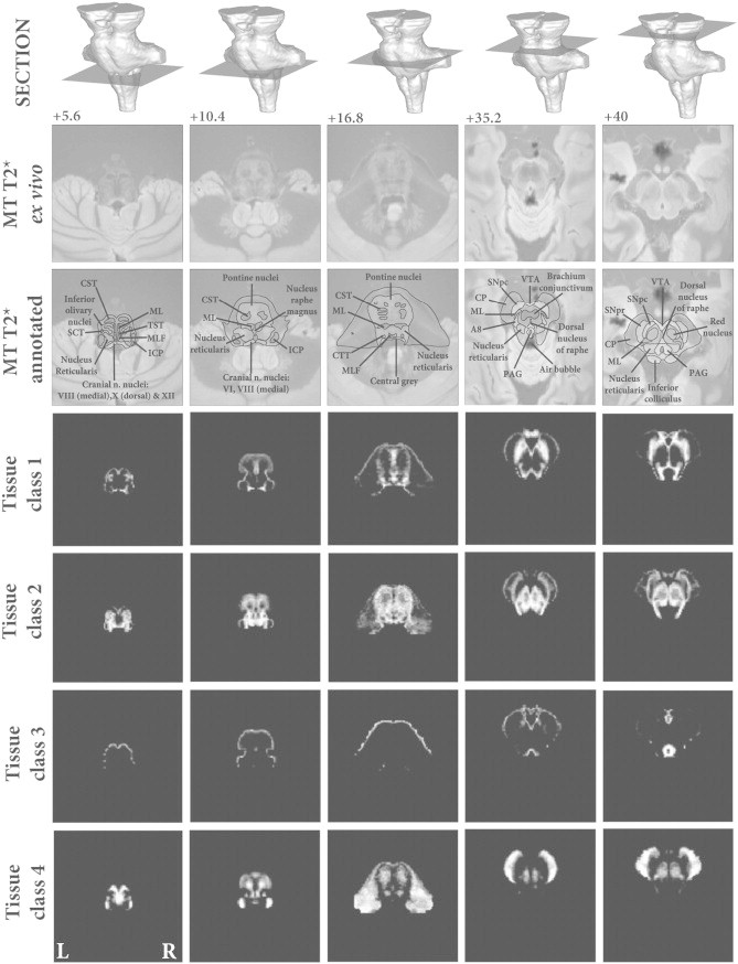
Brainstem tissue probability maps compared against high resolution ex vivo combined MT T2* MRI. Vertical distance from the obex in the z-axis is given in millimeter. Tissue class 1—Brainstem grey matter. Tissue class 2—Reticulated grey matter. Tissue class 3—Periaqueductal grey matter and posterior hypothalamus. Tissue class 4—White matter.

Abbreviations: A8—Dopaminergic centre (approximate location), CP—Cerebral peduncle (anterior to posterior: consisting of frontopontine, corticonuclear, corticospinal and parietotemporal pontine tracts), CST—Corticospinal tract, CTT—Central tegmental tract, ICP—Inferior cerebellar peduncle, ML—Medial lemiscus, MLF—Medial longitudinal fasciculus, PAG—Periaqueductal grey, SCT—Spinocerebellar tract, SNpc—Substantia nigra pars compacta, SNpr—Substantia nigra pars reticulata, TST—Tectospinal tract, VTA—Ventral tegmental area. *Artefact due to fixation.

Fig. 2.

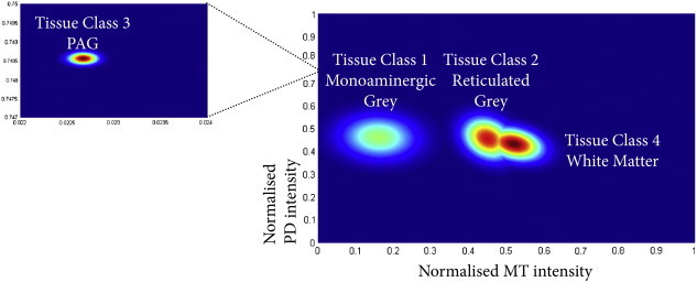
Tissue intensity profiles for the four tissue classes. The MT and PD intensities have been normalised by the maximum value within the brainstem.

3.2. Anatomical validation

Direct validation is difficult without post-mortem data from at least one of the study participants. Additionally, with the exception of the substantia nigra, it is not possible to manually segment many of these structures, as their borders are ill defined on a single image using one MR modality. Here we have taken two approaches to attempt to validate our in vivo data. In Fig. 1, we have taken corresponding sections from the high resolution MT-T2* post mortem data, and labelled the visible structures captured by the TPMs. In an additional step, we also took three representative slices from the brainstem atlas used to label Fig. 1 and projected the TPMs directly onto these images of ex vivo MR microscopy at 9.4 T for the mesencephalon, pons and medulla (Fig. 3 — taken from Duvernoy's Atlas of the Human Brain Stem and Cerebellum with permission). Both show strong correspondence with the recognised brainstem anatomy that can be captured post-mortem at higher resolutions and field-strengths. This indicates that our segmentation algorithm is indeed able to segment brainstem structures at 3 T, and these structures correlate to the accepted MR anatomy. Currently, there is no other approach to achieve this in vivo, particularly at 3 T, limiting any form of analysis in this brain region. Further work is needed to understand how quantitative changes associated with pathology will impact the segmentation algorithm. However, once the tissue priors are achieved, the algorithm becomes no different to the classical segmentation and VBM approaches which have been extensively published, therefore, the presence of disease would not be expected to hamper the segmentation approach.

Fig. 3.

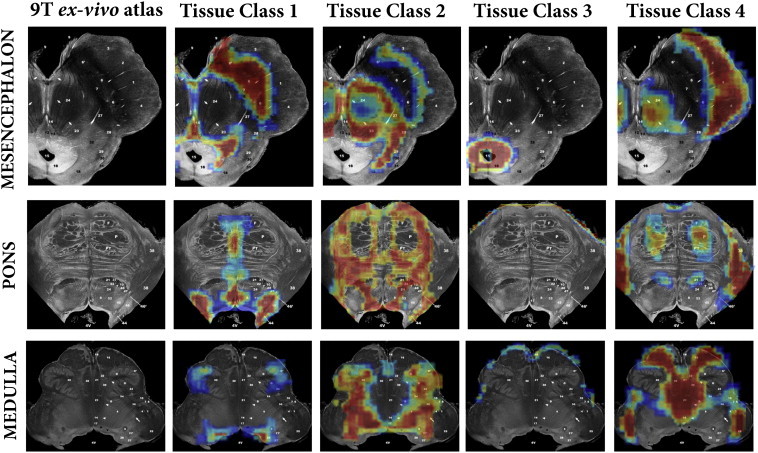
Comparison of calculated tissue classes against three corresponding ex-vivo brainstem sections from “MR microscopy at 9.4 T”.

Taken from Duvernoy's Atlas of the Human Brain Stem and Cerebellum with permission.

3.3. Individual segmentation

The four tissue types were re-warped to a common template using geodesic shooting, resulting in much greater detail captured by the brainstem Jacobians (Fig. 4) compared to the standard approach.

Fig. 4.

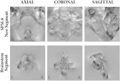
Jacobians for original group warp (top row) and brainstem segmentation group warp (bottom row), highlighting the increased resolution to capture volumetric differences using the latter method.

3.4. Brainstem asymmetries

Significant asymmetries (FWE < 0.05) were found in all the brainstem tissue classes. These are summarised in Fig. 5 and Table 2. Additionally, by thresholding each T-map at FWE < 0.05 and performing a left–right flip, no overlapping regions across all tissue types were present, indicating that the results represent regional expansions in functionally distinct structures. These regions were projected onto a warped MT and PD brainstem and compared against Duvernoy's atlas. Thus, the majority of the regions could be unequivocally identified. The exception was two significant regions that appeared to be present in the motor trigeminal nucleus and medial vestibular nucleus. These were labelled according to the closest associated structure in Duvernoy's atlas, comparing against surrounding visible structures (on both the individual and ex vivo scans) and exiting cranial nerves for localisation. These findings will be considered in detail in the discussion.

Fig. 5.

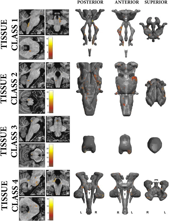
Brainstem regions with significant asymmetries for each tissue class, corrected for multiple comparisons at FWE < 0.05. Row 1—Brainstem grey matter; Row 2—Reticulated grey matter; Row 3—PAG; Row 4—White matter. Renderings display posterior, anterior and superior views of group average TPMs, superior view displayed with anterior posterior axis from bottom to top of the page respectively.

Table 2.

Principle regions with significant asymmetries in the brainstem (FWE < 0.05).

Tissue class	Region (from Duvernoy's atlas)	Asymmetry direction
		Left	Right
1	Inferior olive	+
	Medial vestibular nucleus		+
	Motor trigeminal nucleus		+
2	Nucleus reticularis medullae oblongatae centralis	+
	Inferior pontine nuclei (lateral)	+
	Superior pontine nuclei (lateral)	+
	Trigeminal sensory nucleus/nucleus reticularis pontis		+
3	Inferior PAG	+
	Mid-medial PAG		+
4	Inferior cerebellar peduncle		+
	Pyramid	+
	Corticospinal tract	+
	Middle cerebellar peduncle (inferiolateral)	+
	Middle cerebellar peduncle (superiolateral)		+
	Superior cerebellar peduncle	+

3.5. Tensor based morphometry

These findings mirrored those found using a VBM approach, but only required one statistical test. TBM carried out on the Jacobians, obtained without using the extended brainstem segmentation described above, confirms that this new approach is much more sensitive to detect regional changes within the substance of the brainstem (Fig. 6).

Fig. 6.

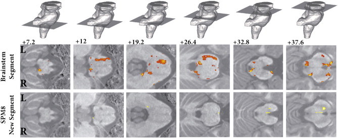
Tissue based morphometry result corrected for multiple comparisons at FWE < 0.05. Top row shows slice position, middle row the new brainstem analysis and bottom row the classical results without brainstem segmentation, highlighting the improvement in statistical sensitivity for regional changes within the substance of the brainstem. Vertical distance from the obex in the z-axis is given in millimeter.

4. Discussion

In this study we have developed a method that allows the internal structure of the human brainstem to be reliably segmented and quantitatively analysed for the first time in vivo. By developing a multimodal segmentation algorithm using mmMoG, brainstem specific tissue probability maps could be generated for four distinct brainstem tissue classes. These probability maps could then be utilised within the pre-existing SPM framework to allow individual segmentation of the brainstem in vivo. Using an accurate diffeomorphic registration algorithm and maintaining the individual segmentations in their native resolution, a highly accurate warping could be achieved with substantial improvement in the estimation of regional deformations. Spatial accuracy was further increased by not smoothing the resulting modulated tissue classes, a step that was permissible for two reasons. Firstly, the brainstem is topologically much simpler than the cortex as there is no gyrification to contend with. Secondly, the diffeomorphic registration method used (geodesic shooting algorithm (Ashburner and Friston, 2011)) is more accurate at aligning this region across subjects. A VBM analysis examining for brainstem asymmetries was primarily undertaken as proof of concept. This demonstrated significant results, which will be discussed further.

4.1. Biophysical interpretation of brainstem tissue classes

In this study we have defined four brainstem tissue classes on the basis of the measured MT and PD parameters. The advantage with using quantitative MRI parameter maps is that they reflect biophysical properties of the underlying tissue more closely than generic MR image. Since the brainstem structures contain axonal tracts and interdispersed nuclei at varying proportion, it is useful to rely on parameters that are sensitive to these features.

Proton density (PD) refers to the concentration of MRI visible hydrogen in mobile water (Tofts, 2003). Since only a small fraction of water is trapped in or otherwise associated to macromolecules, the PD values are therefore a reflection of the tissue water content. Magnetisation transfer (MT) emerges from hydrogen in motionally restricted macromolecules, which do contribute to the MRI signal because of their ultrashort T2. These are, however, weakly coupled to those in water by dipole–dipole interactions and or chemical exchange, and so a selective saturation of the macromolecular magnetisation will be transferred to the water magnetisation and observed as reduced signal (Wolff and Balaban, 2005). The MT maps describe the percentage reduction of water during a single repetition and are not confounded by underlying T1 relaxation and B1 inhomogeneity and more directly related to macromolecular content (Helms et al., 2008). Biologically, the axonal myelin-sheaths are particularly rich in macromolecules and hence MT is a reflection of the quantity of myelin within a voxel. In vivo quantitative MT parameters have been previously shown to be highly correlated with ex vivo measures of myelination and axonal density at post mortem (Schmierer et al., 2004).

Fig. 2 summarises the differences between the tissue classes in terms of measured MT and PD. As expected, white matter (tissue class 4) contains the highest degree of myelination and due to the dense packing of axonal fibres in the brainstem it is therefore unsurprising that there is the lowest amount of free water. Tissue class 2, consisting predominately of reticulated grey matter and pontine nuclei, consists of grey matter that is highly invested or split by ascending and descending white matter fibres, and so forms an intermediate cluster between the white matter and classical grey matter. It is questionable whether MRI can provide sufficiently high spatial resolution to resolve the partial volumes into pure grey and white matter classes, however further work at higher field strengths is required to address this question. In the PAG (tissue class 3), the MT values indicate a very low myelin content and comparatively higher PD compared to the other tissue types. This is consistent with the known ultrastructure of the PAG which is well described as a cell rich, myelin poor region with large numbers of small unmyelinated axons and cells frequently located in small clusters, without interdigitating glial elements (Buma et al., 2004; Carrive, 2004).

Regarding the contribution of each MPM to the final segmentation result, this can also be inferred from Fig. 2, and the value of the multimodal segmentation approach highlighted. The PAG (tissue class 3) was a very distinct tissue class, and on the PD alone the properties of the PAG should make it unique enough to be isolated. This can be seen on an individual PD image (Fig. 7). However the CSF in these images is noisier compared with MT, hence the value of utilising both modalities. With MT images alone, the PAG may be classified with the monoaminergic group due to some overlapping intensity values. With the remaining tissue types, it is apparent that the MT alone can separate the WM and monoaminergic groups (tissue class 1), as has been previously noted by Helms et al. (2009), but would be unable to reliably distinguish WM and reticulated WM, a finding that is apparent with routine segmentation (Fig. 4). In contrast, the proton density alone could isolate GM from WM, but as the tissue contrasts are quite narrow, the result would not be as good as for MT alone.

Fig. 7.

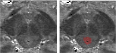
Proton density image showing the PAG.

4.2. Asymmetries in the human brainstem

Asymmetry within the human cortex is a well-established phenomenon. Structurally it can be found at multiple scales from columnar organisation (Seldon, 1982) and cytoarchitectonic boundaries (Rademacher et al., 2001) through white matter tracts (Hasan et al., 2009), small world network topological features (Tian et al., 2011) and cortical thickness (He et al., 2007; Luders et al., 2006). These asymmetries are thought to correlate to numerous lateralised functions, such as handedness (Goble and Brown, 2008), language (Seldon, 1981) and auditory processing (Toga and Thompson, 2003). A number of post-mortem studies have also verified some of these findings, but these are limited due to their labour intensive, time-consuming nature (Schleicher et al., 1999) and may be confounded by numerous practical factors such as fixation methods and measurement techniques (Whitaker and Selnes, 1976). Numerous in vivo MRI studies of cortical asymmetry have been published using a variety of techniques, yet given this abundance of literature there is sparse evidence for asymmetries in the healthy human brainstem. The most likely explanation for the lack of previous evidence is simply that the brainstem is a difficult structure to study. It is constructed of numerous small nuclei with closely associated tracts whose distribution, organisation and function remain poorly understood. The majority of automated MRI based volumetric studies rely on estimating the differences between a structure of interest and a common template. However, as shown in Fig. 4, classical segmentation algorithms treat the brainstem as a single homogenous structure and as such are unable to estimate anything but the most gross anatomical differences. The most reliable structural asymmetry is that of the left corticospinal tract (CST), which has been shown to be larger on the left by post-mortem studies (Rademacher et al., 2001). Quantitative differences in imaging metrics such as FA, but not absolute tract volume, have been found using DTI (Reich et al., 2006; Westerhausen et al., 2007). However, due to the methods used to isolate the CST using DTI, it is unlikely that DTI in isolation can assess the full extent of the brainstem CST volume. Specifically, this is hindered by the need to manually specify seed regions that will exhibit significant inter-individual variability (Rademacher et al., 2001). Additionally, practical tractography issues, such as choice of algorithm, DTI parameters and thresholding level will all limit the accuracy. By utilising the technique within a VBM framework, we have shown multiple asymmetries throughout the brainstem whilst controlling for gender and total brain volume. Importantly, both the corticospinal tract and pyramid were larger on the left, which is in keeping with known anatomy (Kertesz and Geschwind, 1971; Rademacher et al., 2001). In addition to this, our work resulted in novel findings across several brainstem zones. All of the identified regions have also been described as part of the vocal control network (Jürgens, 2002), which given the lateralising effect of Broca's aphasia on the motor control of vocalisation (van Lieshout et al., 2007) could provide a biological basis for the observed asymmetries. Clearly, given that the brainstem is so tightly packed with nuclei responsible for so many functions, these asymmetries could be due to many reasons and further work is needed to investigate whether these findings are related to functional cerebral dominance. However, this example demonstrates the improved sensitivity of the brainstem segmentation scheme, and the wider applicability of this method will be expanded on below.

4.3. Brainstem segmentation — applications

The motivation for developing methods to analyse the brainstem with increased accuracy was driven by the observation that several neurodegenerative diseases have a long prodromal pre-clinical phase before the classical spectrum of diagnostic symptomology becomes evident. An example of this is Parkinson's disease (PD): Currently, it can be argued that neuroimaging is able to detect dopaminergic cell loss in PD approximately four to seven years before clinical motor symptoms are evident (Ponsen et al., 2004). This requires highly specialised techniques such as single photon emission tomography (SPECT) or ¹⁸F-flourodopa positron emission tomography (PET). Not only are these modalities limited by cost and availability (Siderowf and Stern, 2008), they are also invasive, require significant nigro-striatal disease to be present in order to detect a reduction in dopamine, and are subject to significant variability (Michell et al., 2004). However, through large epidemiological and histopathological studies(Hawkes, 2008), it has become clear that the prodromal phase of PD may extend up to 20 or more years before involvement of the nigrostriatal system (Hawkes et al., 2010). This period is characterised by subtle autonomic, olfactory, enteric, sleep, behavioural and cognitive changes (Hawkes et al., 2010; Park and Stacy, 2009; Siderowf and Stern, 2008). Histologically, during this time, there is early involvement of the olfactory cortex and dorsal vagal motor nuclei, before progressive alpha-synuclein deposition ascends the brainstem to involve the raphe group, locus coeruleus and reticular nuclei (Del Tredici et al., 2002; Jellinger, 2009). These are all structures that can be successfully segmented using the proposed methodology, allowing mass univariate methods such as VBM, voxel based quantification (Draganski et al., 2011) or more complicated multivariate analysis to be undertaken with far greater accuracy. Additionally, promising fusions of VBM with machine learning techniques have been previously used to predict the degree of cognitive impairment in Alzheimer's disease based on VBM results (Stonnington et al., 2010). These could easily be implemented with the current brainstem segmentations. Additionally, these segmentations would be well suited to brainstem fMRI, where tissue specific alignment across subjects could reduce noise and increase statistical sensitivity (Beissner et al., 2011; Pattinson et al., 2009). Though the current acquisition time is relatively long (75 min), it was designed as an exploratory analysis. In this study we choose to repeat and average MPM sequence to optimise the SNR, a step that could be omitted in required in future work reducing the acquisition time to 37 min. Additionally, ongoing work is currently applying these methods to a 21-minute, 1 mm isotropic MPM sequence. Whilst not as accurate as the 0.8 mm³ data, it still is a significant advance on currently available techniques, and would be well suited to future patient studies. In short, the proposed method opens the brainstem to a rapidly evolving array of methodological techniques that are well placed to find increasingly specific, non-invasive neuroimaging biomarkers of pre-clinical neurodegenerative diseases and help elucidated the normal function of the brainstem in vivo.

4.4. Brainstem segmentation — limitations

The impact of physiological noise on image quality and the segmentation results has not been explored. However recent in vivo myeloarchitectonic studies of cortical areas using this method illustrate the robustness of the technique and its sensitivity to tissue microarchitecture (Dick et al., 2012; Sereno et al., 2012). Physiological noise has mostly been addressed in the context of fMRI, where image stability is paramount (Glover et al., 2000; Hutton et al., 2011). However these methods cannot be directly implemented in anatomical imaging due to the different types of image acquisition. Phase-navigator correction methods (Barry et al., 2008; Hu and Kim, 1994) might be beneficial although they may reduce the efficiency of the FLASH acquisitions used here. Recent developments involve prospective real-time correction of physiological effects: These include real-time shimming methods for correction of respiratory-induced effects (Van Gelderen et al., 2007) and optical systems for fast prospective correction of subject motion (Zaitsev et al., 2006). These methods are likely to yield a significant reduction of physiological effects on anatomical scans. However, minimal impact on accuracy will be required for use in quantitative MR imaging.

The other principle limitation relates to cluster number selection. In this current study, a range of clustering solutions were investigated and judged visually. This is clearly a non-ideal solution that could be subject to observer bias. However, the problem of cluster number optimisation, despite being extensively studied, is still one that remains problematic and poorly characterised for a number of reasons. The precise definition of a cluster is subjective as it depends entirely on your view-point. The top-down definition seeks to partition a heterogeneous population into more homogenous groups, whereas the bottom-up stance asserts that using local measures of similarity, common groups can be constructed, though equally this could be reformulated as measures of dissimilarity to separate groups. The situation becomes even more complex when attempting to define what a meaningful, or good cluster is, as it depends entirely on the context and users' requirements or aims (Blum, 2009), i.e. “Clustering is in the eye of the beholder” (Estivill-Castro, 2002). This is particularly true in neuroanatomical studies, where established partitions are steeped in historical, often contradictory results (Swanson, 2003). Practically we were extremely cautious in this study not to over-interpret the results, and strived to ensure a biological basis existed for our observations. Over-clustering was deemed to be present when a previously defined, anatomically congruent cluster, broke down into smaller sub-components that did not have an obvious anatomical basis (for example, white-matter sub-clusters or multiple partial volume clusters). Objectively, this was additionally visualised by plotting the tissue intensity profiles. An over-clustered result was evident by highly overlapping plots. However it is likely that more clusters could be found either by utilising greater numbers of scans to estimate the TPMs, obtaining higher resolution data, using higher field strengths or combining with additional modalities (e.g. diffusion, iron-weighted). Future work to develop these techniques will use a combination of these methods to improve on the segmentation results. Additionally, further work is required to investigate the ex vivo biological correlates of measured quantitative MRI parameters such as MT and PD. However, this is a substantial and non-trivial undertaking, and is far beyond the scope of this current study.

5. Conclusion

In conclusion, we have developed a method to allow accurate automated segmentation of the human brainstem in vivo for the first time. We have demonstrated that these segmentations can be used in pre-existing quantitative frameworks such as VBM, and have provided an analysis of brainstem asymmetries as an example. This method would also be well suited to the emergent field of brainstem fMRI (Beissner et al., 2011; Pattinson et al., 2009) to improve registration accuracy between subjects, with a subsequent increase in spatial and statistical sensitivity. Additionally, this technique is particularly important in the search for neuroimaging biomarkers in pre-clinical neurodegenerative diseases such as Parkinson's disease, where it offers several advantages over current modalities. Future work will aim to generalise the multichannel segmentation scheme to the entire cortex, in addition to fusing this technique with diffusion tensor imaging to achieve both a fine grain sub-segmentation of brainstem regions, and also a deeper understanding of brainstem networks and their natural variability in vivo.

References

- Ashburner J., Friston K.J. Voxel-based morphometry—the methods. NeuroImage. 2000;11(6 Pt 1):805–821. doi: 10.1006/nimg.2000.0582. [DOI] [PubMed] [Google Scholar]
- Ashburner J., Friston K.J. Unified segmentation. NeuroImage. 2005;26(3):839–851. doi: 10.1016/j.neuroimage.2005.02.018. [DOI] [PubMed] [Google Scholar]
- Ashburner J., Friston K.J. Diffeomorphic registration using geodesic shooting and Gauss–Newton optimisation. NeuroImage. 2011;55(3):954–967. doi: 10.1016/j.neuroimage.2010.12.049. [DOI] [PMC free article] [PubMed] [Google Scholar]
- Barry R.L., Martyn Klassen L., Williams J.M., Menon R.S. Hybrid two-dimensional navigator correction: a new technique to suppress respiratory-induced physiological noise in multi-shot echo-planar functional MRI. NeuroImage. 2008;39(3):1142–1150. doi: 10.1016/j.neuroimage.2007.09.060. [DOI] [PMC free article] [PubMed] [Google Scholar]
- Beissner F., Deichmann R., Baudrexel S. fMRI of the brainstem using dual-echo EPI. NeuroImage. 2011;55(4):1593–1599. doi: 10.1016/j.neuroimage.2011.01.042. [DOI] [PubMed] [Google Scholar]
- Bishop C.M. Springer; New York: 2006. Pattern Recognition and Machine Learning. [Google Scholar]
- Blum A. NIPS Workshop on Clustering Theory. 2009. Thoughts on clustering. [Google Scholar]
- Buma P., Veening J., Hafmans T., Joosten H., Nieuwenhuys R. Ultrastructure of the periaqueductal grey matter of the rat: an electron microscopical and horseradish peroxidase study. The Journal of Comparative Neurology. 2004;319(4):519–535. doi: 10.1002/cne.903190405. [DOI] [PubMed] [Google Scholar]
- Carrive P. The periaqueductal gray. In: Paxinos G., editor. The Human Nervous System. 2nd edn. Academic Press; San Diego: 2004. pp. 393–423. [Google Scholar]
- Del Tredici K., Rüb U., De Vos R.A., Bohl J.R., Braak H. Where does Parkinson disease pathology begin in the brain? Journal of Neuropathology and Experimental Neurology. 2002;61(5):413–426. doi: 10.1093/jnen/61.5.413. [DOI] [PubMed] [Google Scholar]
- Dick F., Tierney A.T., Lutti A., Josephs O., Sereno M.I., Weiskopf N. In vivo functional and myeloarchitectonic mapping of human primary auditory areas. The Journal of Neuroscience. 2012;32(46):16095–16105. doi: 10.1523/JNEUROSCI.1712-12.2012. [DOI] [PMC free article] [PubMed] [Google Scholar]
- Draganski B., Ashburner J., Hutton C., Kherif F., Frackowiak R.S., Helms G., Weiskopf N. Regional specificity of MRI contrast parameter changes in normal ageing revealed by voxel-based quantification (VBQ) NeuroImage. 2011;55(4):1423–1434. doi: 10.1016/j.neuroimage.2011.01.052. [DOI] [PMC free article] [PubMed] [Google Scholar]
- Estivill-Castro V. Why so many clustering algorithms: a position paper. ACM SIGKDD Explorations Newsletter. 2002;4(1):65–75. [Google Scholar]
- Glover G.H., Li T.Q., Ress D. Image-based method for retrospective correction of physiological motion effects in fMRI: RETROICOR. Magnetic Resonance in Medicine. 2000;44(1):162–167. doi: 10.1002/1522-2594(200007)44:1<162::aid-mrm23>3.0.co;2-e. [DOI] [PubMed] [Google Scholar]
- Goble D.J., Brown S.H. The biological and behavioral basis of upper limb asymmetries in sensorimotor performance. Neuroscience and Biobehavioral Reviews. 2008;32(3):598–610. doi: 10.1016/j.neubiorev.2007.10.006. [DOI] [PubMed] [Google Scholar]
- Grinberg L.T., Rüb U., Ferretti R.E.L., Nitrini R., Farfel J.M., Polichiso L., Gierga K., Jacob-Filho W., Heinsen H. The dorsal raphe nucleus shows phospho-tau neurofibrillary changes before the transentorhinal region in Alzheimer's disease. A precocious onset? Neuropathology and Applied Neurobiology. 2009;35(4):406–416. doi: 10.1111/j.1365-2990.2009.00997.x. [DOI] [PubMed] [Google Scholar]
- Hasan K.M., Kamali A., Kramer L.A. Mapping the human brain white matter tracts relative to cortical and deep gray matter using diffusion tensor imaging at high spatial resolution. Magnetic Resonance Imaging. 2009;27(5):631–636. doi: 10.1016/j.mri.2008.10.007. [DOI] [PubMed] [Google Scholar]
- Hasselblad V. Estimation of parameters for a mixture of normal distributions. Technometrics. 1966:431–444. [Google Scholar]
- Hawkes C.H. The prodromal phase of sporadic Parkinson's disease: does it exist and if so how long is it? Movement Disorders: Official Journal of the Movement Disorder Society. 2008;23(13):1799–1807. doi: 10.1002/mds.22242. [DOI] [PubMed] [Google Scholar]
- Hawkes C.H., Del Tredici K., Braak H. A timeline for Parkinson's disease. Parkinsonism & Related Disorders. 2010;16(2):79–84. doi: 10.1016/j.parkreldis.2009.08.007. [DOI] [PubMed] [Google Scholar]
- He Y., Chen Z.J., Evans A.C. Small-world anatomical networks in the human brain revealed by cortical thickness from MRI. Cerebral Cortex (New York, N.Y.: 1991) 2007;17(10):2407–2419. doi: 10.1093/cercor/bhl149. [DOI] [PubMed] [Google Scholar]
- Helms G., Dathe H., Kallenberg K., Dechent P. High-resolution maps of magnetization transfer with inherent correction for RF inhomogeneity and T1 relaxation obtained from 3D FLASH MRI. Magnetic Resonance in Medicine. 2008;60(6):1396–1407. doi: 10.1002/mrm.21732. [DOI] [PubMed] [Google Scholar]
- Helms G., Draganski B., Frackowiak R., Ashburner J., Weiskopf N. Improved segmentation of deep brain grey matter structures using magnetization transfer (MT) parameter maps. NeuroImage. 2009;47(1):194–198. doi: 10.1016/j.neuroimage.2009.03.053. [DOI] [PMC free article] [PubMed] [Google Scholar]
- Helms G., Brunnquell K., Wrede A., Schulz-Schaeffer W.J., Dechent P. High resolution multi-echo FLASH MRI of fixated human brain with combined magnetization transfer (MT) and T2* weighting. Proceedings of the International Society for Magnetic Resonance in Medicine. 2011;19:2373. [Google Scholar]
- Hu X., Kim S.G. Reduction of physiological noise in functional MRI using navigator echo. Magnetic Resonance in Medicine. 1994;31:495–503. doi: 10.1002/mrm.1910310505. [DOI] [PubMed] [Google Scholar]
- Hutton C., Josephs O., Stadler J., Featherstone E., Reid A., Speck O., Bernarding J., Weiskopf N. The impact of physiological noise correction on fMRI at 7 T. Neuroimage. 2011;57(1):101–112. doi: 10.1016/j.neuroimage.2011.04.018. [DOI] [PMC free article] [PubMed] [Google Scholar]
- Jellinger K.A. Formation and development of Lewy pathology: a critical update. Journal of Neurology. 2009;256(Suppl. 3):270–279. doi: 10.1007/s00415-009-5243-y. [DOI] [PubMed] [Google Scholar]
- Jürgens U. Neural pathways underlying vocal control. Neuroscience and Biobehavioral Reviews. 2002;26(2):235–258. doi: 10.1016/s0149-7634(01)00068-9. [DOI] [PubMed] [Google Scholar]
- Kertesz A., Geschwind N. Patterns of pyramidal decussation and their relationship to handedness. Archives of Neurology. 1971;24(4):326–332. doi: 10.1001/archneur.1971.00480340058006. [DOI] [PubMed] [Google Scholar]
- Luders E., Narr K.L., Thompson P.M., Rex D.E., Jancke L., Toga A.W. Hemispheric asymmetries in cortical thickness. Cerebral Cortex (New York, N.Y.: 1991) 2006;16(8):1232–1238. doi: 10.1093/cercor/bhj064. [DOI] [PubMed] [Google Scholar]
- Lutti A., Hutton C., Finsterbusch J., Helms G., Weiskopf N. Optimization and validation of methods for mapping of the radiofrequency transmit field at 3 T. Magnetic Resonance in Medicine. 2010;64(1):229–238. doi: 10.1002/mrm.22421. [DOI] [PMC free article] [PubMed] [Google Scholar]
- Lutti A., Stadler J., Josephs O., Windischberger C., Speck O. Robust and fast whole brain mapping of the RF transmit field B1 at 7 T. PLoS One. 2012;7(3):e32379. doi: 10.1371/journal.pone.0032379. [DOI] [PMC free article] [PubMed] [Google Scholar]
- Michell A.W., Lewis S.J., Foltynie T., Barker R.A. Biomarkers and Parkinson's disease. Brain: A Journal of Neurology. 2004;127(Pt 8):1693–1705. doi: 10.1093/brain/awh198. [DOI] [PubMed] [Google Scholar]
- Naidich T.P., Duvernoy H.M. illustrated ed. Springer; Wien; New York: 2009. Duvernoy's Atlas of the Human Brain Stem and Cerebellum: High-field MRI: Surface Anatomy, Internal Structure, Vascularization and 3D Sectional Anatomy. [Google Scholar]
- Ortendahl D.A., Hylton N.M. Information processing in medical imaging: proceedings of the 9th conference, Washington, DC, 10–14 June 1985. 1986. p. 62. (Tissue Type Identification by MRI Using Pyramidal Segmentation and Intrinsic Parameters). [Google Scholar]
- Park A., Stacy M. Non-motor symptoms in Parkinson's disease. Journal of Neurology. 2009;256(Suppl. 3):293–298. doi: 10.1007/s00415-009-5240-1. [DOI] [PubMed] [Google Scholar]
- Parvizi J., Damasio A. Consciousness and the brainstem. Cognition. 2001;79(1–2):135–160. doi: 10.1016/s0010-0277(00)00127-x. [DOI] [PubMed] [Google Scholar]
- Pattinson K.T., Mitsis G.D., Harvey A.K., Jbabdi S., Dirckx S., Mayhew S.D., Rogers R., Tracey I., Wise R.G. Determination of the human brainstem respiratory control network and its cortical connections in vivo using functional and structural imaging. NeuroImage. 2009;44(2):295–305. doi: 10.1016/j.neuroimage.2008.09.007. [DOI] [PubMed] [Google Scholar]
- Ponsen M.M., Stoffers D., Booij J., van Eck-Smit B.L., Wolters E.C.h., Berendse H.W. Idiopathic hyposmia as a preclinical sign of Parkinson's disease. Annals of Neurology. 2004;56(2):173–181. doi: 10.1002/ana.20160. [DOI] [PubMed] [Google Scholar]
- Rademacher J., Bürgel U., Geyer S., Schormann T., Schleicher A., Freund H.J., Zilles K. Variability and asymmetry in the human precentral motor system. A cytoarchitectonic and myeloarchitectonic brain mapping study. Brain: A Journal of Neurology. 2001;124(Pt 11):2232–2258. doi: 10.1093/brain/124.11.2232. [DOI] [PubMed] [Google Scholar]
- Reich D.S., Smith S.A., Jones C.K., Zackowski K.M., van Zijl P.C., Calabresi P.A., Mori S. Quantitative characterization of the corticospinal tract at 3 T. AJNR. American Journal of Neuroradiology. 2006;27(10):2168–2178. [PMC free article] [PubMed] [Google Scholar]
- Schleicher A., Amunts K., Geyer S., Morosan P., Zilles K. Observer-independent method for microstructural parcellation of cerebral cortex: a quantitative approach to cytoarchitectonics. NeuroImage. 1999;9(1):165–177. doi: 10.1006/nimg.1998.0385. [DOI] [PubMed] [Google Scholar]
- Schmierer K., Scaravilli F., Altmann D.R., Barker G.J., Miller D.H. Magnetization transfer ratio and myelin in postmortem multiple sclerosis brain. Annals of Neurology. 2004;56(3):407–415. doi: 10.1002/ana.20202. [DOI] [PubMed] [Google Scholar]
- Seldon H.L. Structure of human auditory cortex. II. Axon distributions and morphological correlates of speech perception. Brain Research. 1981;229(2):295–310. doi: 10.1016/0006-8993(81)90995-1. [DOI] [PubMed] [Google Scholar]
- Seldon H.L. Structure of human auditory cortex. III. Statistical analysis of dendritic trees. Brain Research. 1982;249(2):211–221. doi: 10.1016/0006-8993(82)90055-5. [DOI] [PubMed] [Google Scholar]
- Sereno M.I., Lutti A., Weiskopf N., Dick F. Mapping the human cortical surface by combining quantitative T1 with retinotopy. Cerebral Cortex. 2012 doi: 10.1093/cercor/bhs213. [DOI] [PMC free article] [PubMed] [Google Scholar]
- Siderowf A., Stern M.B. Premotor Parkinson's disease: clinical features, detection, and prospects for treatment. Annals of Neurology. 2008;64(Suppl. 2):S139–S147. doi: 10.1002/ana.21462. [DOI] [PubMed] [Google Scholar]
- Simic G., Stanic G., Mladinov M., Jovanov-Milosevic N., Kostovic I., Hof P.R. Does Alzheimer's disease begin in the brainstem? Neuropathology and Applied Neurobiology. 2009;35(6):532–554. doi: 10.1111/j.1365-2990.2009.01038.x. [DOI] [PMC free article] [PubMed] [Google Scholar]
- Stonnington C.M., Chu C., Klöppel S., Jack C.R., Ashburner J., Frackowiak R.S., Alzheimer Disease Neuroimaging Initiative Predicting clinical scores from magnetic resonance scans in Alzheimer's disease. NeuroImage. 2010;51(4):1405–1413. doi: 10.1016/j.neuroimage.2010.03.051. [DOI] [PMC free article] [PubMed] [Google Scholar]
- Swanson L.W. The amygdala and its place in the cerebral hemisphere. Annals of the New York Academy of Sciences. 2003;985(1):174–184. doi: 10.1111/j.1749-6632.2003.tb07081.x. [DOI] [PubMed] [Google Scholar]
- Tian L., Wang J., Yan C., He Y. Hemisphere- and gender-related differences in small-world brain networks: a resting-state functional MRI study. NeuroImage. 2011;54(1):191–202. doi: 10.1016/j.neuroimage.2010.07.066. [DOI] [PubMed] [Google Scholar]
- Tofts P. John Wiley & Sons Inc.; 2003. Quantitative MRI of the Brain: Measuring Changes Caused by Disease. [Google Scholar]
- Toga A.W., Thompson P.M. Mapping brain asymmetry. Nature Reviews Neuroscience. 2003;4(1):37–48. doi: 10.1038/nrn1009. [DOI] [PubMed] [Google Scholar]
- Van Gelderen P., De Zwart J.A., Starewicz P., Hinks R.S., Duyn J.H. Real-time shimming to compensate for respiration-induced B0 fluctuations. Magnetic Resonance in Medicine. 2007;57(2):362–368. doi: 10.1002/mrm.21136. [DOI] [PubMed] [Google Scholar]
- Van Lieshout P.H., Bose A., Square P.A., Steele C.M. Speech motor control in fluent and dysfluent speech production of an individual with apraxia of speech and Broca's aphasia. Clinical Linguistics & Phonetics. 2007;21(3):159–188. doi: 10.1080/02699200600812331. [DOI] [PubMed] [Google Scholar]
- Weiskopf N., Lutti A., Helms G., Novak M., Ashburner J., Hutton C. Unified segmentation based correction of R1 brain maps for RF transmit field inhomogeneities (UNICORT) NeuroImage. 2011;54(3):2116–2124. doi: 10.1016/j.neuroimage.2010.10.023. [DOI] [PMC free article] [PubMed] [Google Scholar]
- Westerhausen R., Huster R.J., Kreuder F., Wittling W., Schweiger E. Corticospinal tract asymmetries at the level of the internal capsule: is there an association with handedness? NeuroImage. 2007;37(2):379–386. doi: 10.1016/j.neuroimage.2007.05.047. [DOI] [PubMed] [Google Scholar]
- Whitaker H.A., Selnes O.A. Anatomic variations in the cortex: individual differences and the problem of the localization of language functions. Annals of the New York Academy of Sciences. 1976;280:844–854. doi: 10.1111/j.1749-6632.1976.tb25547.x. [DOI] [PubMed] [Google Scholar]
- Wolff Steven D., Balaban Robert S. Magnetization transfer contrast (MTC) and tissue water proton relaxation in vivo. Magnetic Resonance in Medicine. 2005;10(1):135–144. doi: 10.1002/mrm.1910100113. [DOI] [PubMed] [Google Scholar]
- Yushkevich P.A., Piven J., Hazlett H.C., Smith R.G., Ho S., Gee J.C., Gerig G. User-guided 3D active contour segmentation of anatomical structures: significantly improved efficiency and reliability. NeuroImage. 2006;31(3):1116–1128. doi: 10.1016/j.neuroimage.2006.01.015. [DOI] [PubMed] [Google Scholar]
- Zaitsev M., Dold C., Sakas G., Hennig J., Speck O. Magnetic resonance imaging of freely moving objects: prospective real-time motion correction using an external optical motion tracking system. NeuroImage. 2006;31(3):1038–1050. doi: 10.1016/j.neuroimage.2006.01.039. [DOI] [PubMed] [Google Scholar]
- Zrinzo L., Zrinzo L.V., Tisch S., Limousin P.D., Yousry T.A., Afshar F., Hariz M.I. Stereotactic localization of the human pedunculopontine nucleus: atlas-based coordinates and validation of a magnetic resonance imaging protocol for direct localization. Brain: A Journal of Neurology. 2008;131(Pt 6):1588–1598. doi: 10.1093/brain/awn075. [DOI] [PubMed] [Google Scholar]