Computer-aided detection of radiation-induced cerebral microbleeds on susceptibility-weighted MR images

Abstract

Recent interest in exploring the clinical relevance of cerebral microbleeds (CMBs) has motivated the search for a fast and accurate method to detect them. Visual inspection of CMBs on MR images is a lengthy, arduous task that is highly prone to human error because of their small size and wide distribution throughout the brain. Several computer-aided CMB detection algorithms have recently been proposed in the literature, but their diagnostic accuracy, computation time, and robustness are still in need of improvement. In this study, we developed and tested a semi-automated method for identifying CMBs on minimum intensity projected susceptibility-weighted MR images that are routinely used in clinical practice to visually identify CMBs. The algorithm utilized the 2D fast radial symmetry transform to initially detect putative CMBs. Falsely identified CMBs were then eliminated by examining geometric features measured after performing 3D region growing on the potential CMB candidates. This algorithm was evaluated in 15 patients with brain tumors who exhibited CMBs on susceptibility-weighted images due to prior external beam radiation therapy. Our method achieved heightened sensitivity and acceptable amount of false positives compared to prior methods without compromising computation speed. Its superior performance and simple, accelerated processing make it easily adaptable for detecting CMBs in the clinic and expandable to a wide array of neurological disorders.

Highlights

► A computer-aided method to detect cerebral microbleeds (CMBs) on MRI is proposed. ► The method is based on 2D fast radial symmetry transform and 3D region growing. ► The method was evaluated for radiation-induced CMBs in patients with brain tumors. ► The evaluation has shown the high sensitivity and fast computation of the method.

1. Introduction

Cerebral microbleeds (CMBs) are small, frequently perivascular collections of brain parenchymal hemosiderins induced by prior hemorrhage. On MR T2*-weighted gradient echo (GRE) magnitude images, CMBs appear as small, rounded, hypointense lesions of variable size due to susceptibility-related signal loss within iron-containing hemosiderins that accumulate paramagnetic ferric atoms (Charidimou and Werring, 2011; Cordonnier et al., 2007; Greenberg et al., 2009). Since the susceptibility effect scales linearly with magnetic field strength, the contrast of CMBs is greatly enhanced by higher field strengths (e.g., at 3 T or 7 T) and susceptibility-weighted imaging (SWI) (Ayaz et al., 2010; Conijn et al., 2011; Nandigam et al., 2009). Because this heightened contrast has facilitated the detection of CMBs, there is a growing interest in exploring their diagnostic and prognostic values in diseases such as cerebral amyloid angiopathy (CAA) (Greenberg et al., 1999), stroke (Cordonnier et al., 2007; Fiehler, 2006; Werring et al., 2005); neurodegenerative disorders (Cordonnier and van der Flier, 2011), traumatic brain injury (TBI) (Scheid et al., 2003), and radiation therapy-induced injury in patients with gliomas (the most common brain tumors) (Lupo et al., 2012). Although their putative role in neurocognitive function and implications for clinical management are still being evaluated (Charidimou and Werring, 2011; Cordonnier et al., 2007; Greenberg et al., 2009), there is accumulating evidence that CMBs reflect the severity of microvascular damage in the brain due to microangiopathy (Vernooij et al., 2008), TBI (Scheid et al., 2003), or radiation therapy (Lupo et al., 2012).

Visual inspection of CMBs on MR images is especially difficult due to their small size (with radii often < 2 mm for radiation-induced CMBs) and wide distribution throughout the brain. In CAA and following cranial radiation, the sheer large number of CMBs can render manual lesion counting impractical or impossible. Detection is further confounded by the presence of normal anatomical structures with heightened magnetic susceptibility that mimic the appearance of CMBs on T2*-sensitive sequences, such as deoxyhemoglobin-containing intracranial veins. These characteristics make the identification of CMBs a lengthy and arduous task that is prone to human error and substantial intra-rater and inter-rater variability (Cordonnier et al., 2009; Gregoire et al., 2009). An automatic, computer-aided CMB detection method that can both minimize the burden of visual inspection and improve the accuracy of detection of CMBs is therefore highly desirable.

Several methods have been proposed for CMB detection (Barnes et al., 2011; Kuijf et al., 2012; Seghier et al., 2011). Seghier et al. (2011) implemented an intensity-based statistical classification algorithm in which T2*-weighted magnitude images are first registered to a standard template that maps voxelwise probabilities of individual brain structures such as gray matter, white matter, cerebral spinal fluid, and CMBs. Gaussian mixture modeling is then applied to distinguish CMBs from other brain structures. They identified patients with CMBs at a sensitivity of 77% and a detection rate of 50% for total true CMBs without giving the number of false positives. Barnes et al. (2011) proposed a technique for intensity-based local statistical thresholding that assumes the Gaussian distribution of background tissue in a small region and then identifies hypointense CMBs as outliers. False positives were reduced by constructing a support vector machine that incorporates shape, size and intensity as features for each hypointense region to distinguish CMBs from mimics. They achieved a detection sensitivity of 81.7% with 107.5 false positives per patient. Kuijf et al. (2012) developed an algorithm for CMB detection based on the fast radial symmetry transform (FRST), which enhances local objects with spherical or near-spherical geometry (Loy and Zelinsky, 2003). By using the transform, the algorithm achieved a detection rate of 71.2% with 17.2 false positives per patient.

Despite the reported success of these computer-aided methods for detecting CMBs, there remains a need to improve diagnostic accuracy with simpler processing, less computation time, and greater robustness in the presence of anatomic distortion such as brain tumors, resections, and infarcts. In addition, all of the above methods are designed to detect CMBs on T2*-weighted magnitude or SWI images without minimum intensity projection (mIP) processing, which helps distinguish CMBs from hypointense veins and is used in clinical practice for visual inspection of CMBs (Lupo et al., 2012), even by the groups who have developed these automated methods (Ayaz et al., 2010; de Bresser et al., in press). Direct adaptation of their methods for CMB detection on mIP images may be nontrivial as the original geometric coordinates and characteristics of CMB vary after the mIP process, rendering some of the prerequisites associated with these features invalid for these methods.

In this study, we propose a new approach for CMB detection with higher sensitivity and faster computation than has been previously reported, even in the presence of anatomic disease. This approach aims to detect CMBs on mIP SWI images, and the detection process is divided into two main steps: 1) initial putative CMB detection using the 2D FRST, 2) subsequent false positive reduction by characterizing geometric features of putative CMBs through region growing. Although the FRST has already been used to detect CMBs on T2*-weighted magnitude images (Kuijf et al., 2012), the transform was performed in 3D, which requires isotropic image acquisition, and even a perfectly spherical paramagnetic object under isotropic acquisition becomes elongated along the direction of the main magnetic field on T2*-weighted images because the profile of its perturbation of the external field is not spherical (Schenck, 1996). Also, the transform has been modified and utilized in new ways in our implementation. To illustrate the effectiveness of the proposed approach, we applied the method to a series of patients with CMBs induced by radiation treatment for resected gliomas.

2. Methods

2.1. CMB detection algorithm

The proposed algorithm can be divided into two primary steps: 1) identification of putative CMBs using 2D FRST; and 2) false positive reduction of putative CMBs identified in the first step using 3D region growing followed by geometric feature examination. A flowchart depicting the steps for this algorithm is given in Fig. 1. Details of the implementation will be described in the following sections.

Fig. 1.

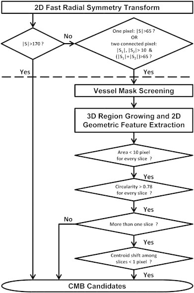
Schematic diagram for the proposed CMB detection algorithm and selected optimized parameters. (S refers to the intensity of FRST map; the processing above the dashed line belongs to the step of initial putative CMB detection, while the below belongs to the step of false positive reduction.)

2.1.1. Detection of putative CMBs using 2D FRST

2.1.1.1. FRST

The inherently circular morphology of CMBs on SWI images makes lesion geometry an ideal feature for automated detection. For this purpose, a modified version of the FRST that was developed by Loy and Zelinsky (2003) was adopted in our algorithm. Our goal in this initial step was to select a set of parameters that would identify the greatest possible number of true microbleeds, regardless of the number of false positives.

FRST is a gradient-based transform that begins with a computation of the gradient of each pixel using the 3 × 3 Sobel operator. If a pixel p lies on the edge of a circular disk, then the direction of its gradient g(p) is orthogonal to the edge, pointing to (if the circular disk is hyperintense) or away from (if the disk is hypointense) the center of the circle. The pixel that is at a distance n pixel away from p along the direction of g(p) is defined as a positively-affected pixel, whereas the pixel that is at a distance n pixel away from p along the direction opposite to that of g(p) is defined as a negatively-affected pixel. Since CMBs are hypointense objects on MR images, we only need to consider negatively-affected pixels, whose coordinates are given by

$$p_{-\mathit{ve}}\left(\mathbf{p}\right)=\mathbf{p}-\mathrm{round}\left(\frac{\mathbf{g}\left(\mathbf{p}\right)}{‖\mathbf{g}\left(\mathbf{p}\right)‖}\right)n,$$

where “round” rounds each vector element to the nearest integer and n is the radius of the circular features to be detected. Since there is no prior knowledge about the radius of the circular object to be detected, the transform is performed at a set of radii n ∈ N. At each radius, an orientation projection image O_n and a magnitude projection image M_n are generated as the following:

$$\begin{array}{l}{O}_n\left({\mathbf{p}}_{-\mathit{ve}}\left(\mathbf{p}\right)\right)=O_{n\_\mathit{prev}}\left({\mathbf{p}}_{-\mathit{ve}}\left(\mathbf{p}\right)\right)-1,\\ M_n\left({\mathbf{p}}_{-\mathit{ve}}\left(\mathbf{p}\right)\right)=M_{n\_\mathit{prev}}\left({\mathbf{p}}_{-\mathit{ve}}\left(\mathbf{p}\right)\right)-‖g\left(P\right)‖.\end{array}$$

The initial value of each pixel in O_n and M_n is set to zero. For each negatively-affected pixel, the value of that pixel p_−ve in the O_n and M_n is decreased by 1 and  ‖g(P)‖  from O_{n_prev} (previous O_n) and M_{n_prev} (previous M_n), respectively. All edge pixels on the boundary of a hypointense circle with a radius of n will have their negatively-affected pixels located at the center of the circle, highlighting the central pixel in O_n and M_n. To prevent corruption by noise, gradient magnitudes smaller than the 95th percentile (background pixels on our SWI images have gradient of zero) were ignored in our experiments when computing O_n and M_n. This threshold was found to adequately suppress background noise while maintaining reasonable sensitivity to CMBs with low contrast.

Once the O_n and M_n are calculated, the radial symmetry contribution at radius n can be defined as:

$$F_n\left(\mathbf{p}\right)=\frac{M_n\left(\mathbf{p}\right)}{k_n}{\left(\frac{\left|{\tilde{O}}_n\left(\mathbf{p}\right)\right|}{k_n}\right)}^{\alpha }$$

where

$${\tilde{O}}_n\left(\mathbf{p}\right)=\{\begin{array}{c}\hfill O_n\left(\mathbf{p}\right)\mathrm{if}{O}_n\left(\mathbf{p}\right)<k_n\hfill \\ \hfill k_n\mathrm{otherwise}.\hfill \end{array}$$

k_n is a scaling factor used to normalize O_n and M_n across different radii such that the symmetry map of objects with different size can be represented on a similar scale. The α parameter is used to characterize radial strictness, with higher values enhancing features with radial symmetry (i.e. dots) and attenuating features without radial symmetry (i.e. lines). The full transform map is computed by summing the symmetry contribution over all the radii: S = ∑ _n ∈ NF_n.

In the original transform proposed by Loy and Zelinsky (2003), F_n has to be convolved with a Gaussian kernel in order to spread the influence of the p_−ve as a function of the radius n. Because we are only interested in knowing the center location of each potential CMB during the initial detection step, this convolution is skipped in our algorithm. In addition, instead of initializing O_n with zero, a small negative value was used as the initial value for each pixel in O_n. This modification increases the weight given to small radii over the other radii and thus improves the sensitivity of the transform to small circular objects (Riccardi, 2006). An example of a slice of mIP SWI image and its 2D FRST map are shown in Fig. 2(a) and (b), respectively.

Fig. 2.

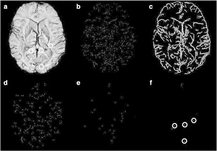
Example outputs from 2D FRST and 3D region growing. (a) A representative mIP SWI slice from a glioma patient with 4 CMBs (circles) on the displayed slice. (b) FRST map before thresholding. (c) Vessel mask, highlighting vessels and the edge of the brain. (d) FRST map after thresholding but before applying the vessel mask in (c). (e) FRST map after thresholding and masking (c). The bright foci are the centers of potential CMBs. Compared to the map in (d), the number of putative CMB candidates are greatly reduced by applying the mask. (f) The final output of detected CMB candidates after false positive reduction. All 4 CMBs (circles) were detected with 3 false positives left.

2.1.1.2. Intensity screening of FRST map

Pixels that have transform value S with absolute value larger than an empirical threshold t₁ on the FRST map are directly identified as CMB candidates without 3D region growing. This upper bound defines hypointense regions with relatively large radius and high contrast, consisting primarily of true CMBs and very few false positives. To recover CMBs with smaller radii and lower contrast, pixels with |S| falling between t₁ and a lower threshold t₂ (also determined empirically) are also considered as candidate CMBs. While a smaller absolute value for the lower threshold t₂ boosts sensitivity to true CMBs that are intended to be recovered, this choice for the parameter also results in a larger number of false positive lesions. The majority of these false positive CMBs are subsequently removed by performing the steps illustrated in Fig. 1. To overcome the uncertainty introduced by partial volume averaging of sub-millimeter CMBs, we also consider regions with |S| < t₂ but impose two additional constraints: 1) the region must contain two connected pixels with both of their absolute values of S larger than t₃ (with t₃ < t₂); and 2) the absolute value of the sum of the two connected pixels is larger than t₂. This step prevents the elimination of true CMBs with less circular morphology where the peak of the FRST is blurred into neighboring pixels. The rational for how these threshold values were determined can be found in the Parameter selection section.

2.1.2. False positive reduction

The number of false positives generated during the initial detection step of our algorithm is large due to the low thresholds t₂ and t₃ used for the FRST map to intentionally maximize detection sensitivity in the first step. Stringent false positive reduction via the employment of a vessel mask, 3D region growing, and geometric feature examination is performed to eliminate the majority of these misidentified CMBs before final visual evaluation.

2.1.2.1. Vessel mask screening using FRST outputs

Beyond its capability in the enhancement of the center of circular objects, we also found empirically that FRST helped to reduce false positives on original maps. Specifically, the orientation projection map O₁ (O_n computed at n = 1) emphasizes vessels and the edges of brain, regions where CMB mimics are typically found. The projection map O₁ can therefore be used to create a binary mask in which a pixel value is 1 if its O₁ decreased at least by one from its initial value (denoting vessels and the edges of brain), or 0 otherwise. The final mask is generated after removing binary regions with an area smaller than 25 pixels (a value that was comparable to the observed maximal CMB area). Only smaller CMBs undergo this vessel mask screening to prevent true large CMBs from being eliminated by the mask. Application of this mask to the FRST maps will reduce the number of initial false positives as shown in Fig. 2(c–e).

2.1.2.2. 3D region growing

Because all thresholds used in the initial detection are applied to the 2D FRST map slice by slice, it is likely that a putative CMB will be detected multiple times on different slices. The central seed point from which to begin region growing is first determined by finding the minimum intensity of a 3D locally connected region (26-connectivity) that contains all detected pixels of a putative CMB on mIP SWI images. 3D region growing is subsequently performed from this center to neighboring pixels based on 26-connectivity if |I_n − I_s| < MID, where I_n, I_s and MID are the intensity of the neighboring pixels, seed point intensity, and the maximum intensity difference between pixels, respectively. The growing stops when either |I_n − I_s| > MID, or the distance from the seed point exceeds a maximum grown radius both in-plane (MP) and in the slice direction (MS).

2.1.2.3. 2D geometric feature examinations

After 3D region growing, 2D geometric features were extracted on every slice of the grown region. We chose to quantify 2D measures of area and circularity rather than 3D measures of volume and sphericity because the latter are distorted after mIP processing. Area is measured as the total number of pixels that comprise a putative CMB and is utilized to remove false positives corresponding to large objects. Circularity (C) is defined as the ratio of the area of the CMB shape to the area of a circle having the same perimeter (C = (4π × area) / perimeter²). Circularity measures range from 0 to 1, with circles having a value of 1 and lines a value approaching 0. This parameter removes objects that are irregular or elongated such as vessels. For each of the remaining CMBs, a centroid is then calculated at each slice location in order to remove false positives with slices that are shifted away from the central axis, such as transverse vessels that have a circular cross-section on 2D slices.

2.1.3. Parameter selection

2.1.3.1. FRST

Three parameters of the FRST, k_n, n, and α, were empirically selected to achieve the highest possible sensitivity to CMBs. In our experiments, the normalization factor k_n was set to 5 for n = 1 and 8 for n > 1. These values are less than the values suggested by Loy and Zelinsky (2003), but improve the sensitivity of the transform to smaller CMBs. As suggested by Kuijf et al. (2012), α was set to 3, and the set of radii n was allowed to vary from 1 to 3 pixels in order to encompass the majority of our CMBs.

2.1.3.2. Thresholding of FRST map

In order to first select easily identifiable true CMBs with |S| >= t₁, which have relatively large radius and high contrast, a sufficiently high threshold should be used for t₁. We therefore reviewed FRST outputs from multiple representative CMBs of intermediate size, and based on this review, empirically chose the threshold to be 170. In contrast, a sufficiently low threshold should be used for t₂ and t₃ to detect CMBs that have a smaller radius and lower contrast such that pixels with |S| >= t₂ but <=t₁ are also considered as potential CMB candidates. To determine the values for t₂ and t₃, the FRST outputs from representative CMBs with extremely low contrast or small radii were investigated, and values of 65/10 were chosen for t_2/t₃ to ensure that nearly all true CMBs were included after thresholding. For any two connected pixels in the FRST map, a potential CMB is selected only if their combined |S| is larger than t₂ and each individual |S| is greater than t₃. Because the t₁ value of 170 was set solely to achieve heightened detection specificity while a t_2/t₃ value of 65/10 was determined to maximize detection sensitivity, the empirical estimation of these threshold parameters from representative CMBs is feasible without the risk of over-training of these parameters.

2.1.3.3. Volume control in 3D region growing

The main requirement for our region growing algorithm was the ability to sufficiently grow the extent of the initial region so that enough elongation is achieved to distinguish small vessels from CMBs, while preventing the generation of false negatives adjacent to neighboring hypointense regions. The parameters that control the extent of the grown region MP and MS, were determined based on prior knowledge of CMB size (whose typical maximal diameter is approximately 6 pixels or 3 mm in diameter) and the fact that only smaller CMB candidates will undergo region growing. The values we selected for MS and MP allowed a region to maximally traverse 3 image slices (6 mm) with a maximum diameter of 10 pixels (5 mm), respectively, both of which have exceeded the typical maximal size of CMBs we investigated. While an acceptable threshold for MP and MS can be easily determined, receiver operating characteristic (ROC) curve analysis with patients from a training set was necessary to establish a threshold for the MID between a grown pixel and the seed point, due to its inherently greater variability because the standard deviation of pixel intensity within CMBs and vessels can vary with image contrast and anatomical location. Based on the ROC curve analysis illustrated in Fig. 3, a MID of 60 (jointly considered with C) resulted in the best overall detection performance based on minimizing distance to the upper left corner and was thus utilized in the final parameter set when validating our algorithm.

Fig. 3.

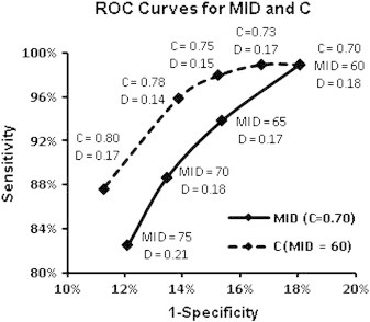
ROC curves constructed using the data from a training set that contains 5 patients and 116 true CMBS. The curves were used to determine cutoff thresholds for maximal intensity difference (MID) between the seed point and the final grown point after region growing (solid line; assuming C = 0.70), and circularity in geometric feature examination (dashed line; assuming MID = 60). When points on both curves are considered all together, C = 0.78 and MID = 60 are the optimal cutoffs in terms of their shortest distance (D = 0.14) to the upper left corner (Note the scales of horizontal and vertical axes are not equal). The distance was also calculated for MID = 65 with C = 0.75 and MID = 65 with C = 0.78, but neither combination gave a distance that was less than 0.14. Thus, the cutoff values for MID and C were set to 60 and 0.78, respectively.

2.1.3.4. Determination of thresholds for geometric feature extraction

Similarly to region-growing parameters MP and MS, the maximum area on any 2D slice for a given CMB was also determined by its physical size. A conservative value of 10 pixels, which corresponds to a diameter of 3.6 pixels or 1.8 mm, was selected. A centroid shift of 1 pixel (0.5 m) was allowed in either direction to account for partial-voluming with discretization. CMB candidates with parameter values larger than these thresholds are removed. Because true CMBs that are less than 1 mm in diameter can appear more rectangular than circular in shape as limited by our pixel resolution, the range of circularity values was quite large. As a result, the threshold for circularity was determined by constructing and analyzing ROC curves jointly for MID and C as shown in Fig. 3. When all points on both curves were considered together, C = 0.78 and MID = 60 were optimal cutoffs.

2.2. Validation of CMB detection algorithm in patients

2.2.1. Patient population

Fifteen patients with gliomas, who had undergone T2*-weighted MR imaging at our research center, were retrospectively selected to train parameters and evaluate the performance of our algorithm. To be eligible for this study, patients had to have received fractionated external beam radiation therapy, which damages microvasculature in normal brain parenchyma and results in the formation of CMBs. Because CMBs are not typically observed in the initial 1 ~ 2 years following cranial irradiation (Lupo et al., 2012), patients were only included if radiation was completed at least 2 years prior to MR imaging. Finally, patients were only included if they had at least 10 potential CMBs on initial screening, as these cases are where automated methods are most desired. The patients were randomly divided into two sets: a training set that included 5 patients and a test set that included 10 patients. The training set was used to construct ROC curves for C and MID to determine their optimal values, while the test set was used to evaluate the performance of the algorithm.

2.2.2. MR Imaging

MR images were acquired on a GE 3 T whole-body system (GE Healthcare, Waukesha, WI) with an 8-channel phased array receive coil (Nova Medical, Wilmington, MA). High resolution T2*-weighted imaging using a 3D flow-compensated spoiled gradient echo sequence was performed using TE/TR = 28/56 ms, flip angle 20°, 24 cm FOV, in-plane resolution of 0.5 × 0.5 mm, 2 mm slice thickness and a total slice number of 40 targeted to the area of glioma resection. A GRAPPA-based parallel imaging acquisition was implemented with a 2-fold acceleration factor in order to keep the total acquisition time under 7 min.

2.2.3. Image reconstruction and preprocessing

Standard SWI post-processing techniques were applied to the reconstructed k-space data for each coil, and then combined and intensity corrected (Haacke et al., 2004; Lupo et al., 2009). The skull and background were removed from reconstructed images by applying a brain mask created from the combined magnitude image with FSL's brain extraction tool software (Smith, 2002). Images were then normalized to an intensity range of 0–255 using 0 and the 98th percentile intensity of original images as the original minimum and maximum intensity, respectively. Finally, minimum intensity projection images through 8 mm-thick slabs (4 slices), with a 6 mm-thick (3 slices) overlap between each consecutive projection, were generated from the intensity-normalized images and used for CMB identification.

2.2.4. Visual assessment of true CMB burden

CMBs were counted by two raters, one subspecialty-certified neuroradiologist (CPH) and one trained reader (JML). CMBs were counted independently by each reader, and discrepancies were resolved by consensus review. Raters initially counted CMBs using the proposed algorithm with parameters set for high sensitivity but low specificity. Both raters distinguished true CMBs from false-positive CMBs and additionally searched for true CMBs missed by the algorithm. The algorithm developer (WB) was blinded to the true lesion counts as determined by the interpreters, while both raters were blinded to the parameter selection. Our way of counting CMBs is driven by the finding, observed both by Kuijf et al. (2012) and by our initial experience in developing the algorithm, that an automated technique may be able to detect extra true CMBs apart from those identified by visual inspection alone. A gold standard of true CMBs, therefore, would be better constructed by comprising CMBs identified not only by visual inspection but also by automated detection.

CMBs in our gold standard were further divided into two groups by the interpreters: definite and possible. Definite CMBs were defined as those lesions with sufficient circular shape and hypointensity to be considered unambiguously as CMBs and not mimics on visual analysis. Possible CMBs were characterized by one or more of following deviations from definite CMBs: 1) less circular shape; 2) less tissue contrast; 3) a location or appearance that made it difficult to distinguish with confidence as representing a mimic such as a small “end-on” cortical vessel. Our criteria to scoring CMBs into the two categories are similar to those used in the literature (Conijn et al., 2011; de Bresser et al., in press; Gregoire et al., 2009). In addition, regions where CMBs are unlikely to occur, such as the ventricles and tumor cavity, as well as areas within a 5 mm margin of the tumor cavity (which were frequently lined by confounding post-operative blood products) were excluded from the assessment.

3. Results

A total of 420 true CMBs were detected from 15 patients, of which 116 were from 5 patients in the training set and 304 were from 10 patients in the test set. Among the CMBs from the test set, 153 were classified as “Definite” and 151 as “Possible”. The definite CMBs had a larger average size (1.16 mm in diameter) and lower average minimum intensity (35.7) than possible CMBs (0.92 mm and 68.4). The minimum diameter detected was 0.57 mm (1.13 pixel) and the largest 2.46 mm (4.92 pixels). The number, diameter, and minimum intensity of these CMBs from the test set are listed in Table 1.

Table 1.

Characteristics of true CMBs identified from 10 patients in the test set.

	Number			Diameter	Minimum intensity
CMBs	Total	Mean	Range	Mean (mm/pixel)	Mean	Max
Definite	153	15.3	2–47	1.16/2.31	35.7	118
Possible	151	15.1	5–36	0.92/1.84	68.4	147
All	304	30.4	8–83	1.04/2.08	52.0	147

Table 2 summarizes the performance of the algorithm on the test set, which was able to correctly identify 263 of 304 total true CMBs, resulting in a sensitivity of 86.5%. Of these correctly identified CMBs, 16.7% (all definite) were directly identified after the FRST and did not undergo region growing and geometric feature examinations. Separating CMBs into two categories improved the sensitivity of definite CMBs to 95.4%, while, as expected, our algorithm was less sensitive (77.5%) to possible CMBs. Fig. 4 shows several examples of true CMBs detected by various steps of the algorithm. Of the 41 CMBs that were missed, 12 had low contrast with mean minimum intensity of 116.8 and a mean |S| of 56, which was out of the selection range on the FRST maps. After applying the vessel mask to the FRST maps, 6 more true CMBs were lost because of their close proximity to vessels or tissue boundaries. The remaining 23 missed CMBs were removed in region growing and geometric feature examinations. A representative example of false negatives created at each of these steps is shown in Fig. 5.

Table 2.

CMB detection algorithm performance evaluated on the test set.

CMB	True	Detected	Sensitivity	False negative			False positive
				FRST	application of FP mask	Region growing
Definite	153	146	95.4%	0	1	6	–
Possible	151	117	77.5%	12	5	17	–
Total	304	263	86.5%	12	6	23	449

Fig. 4.

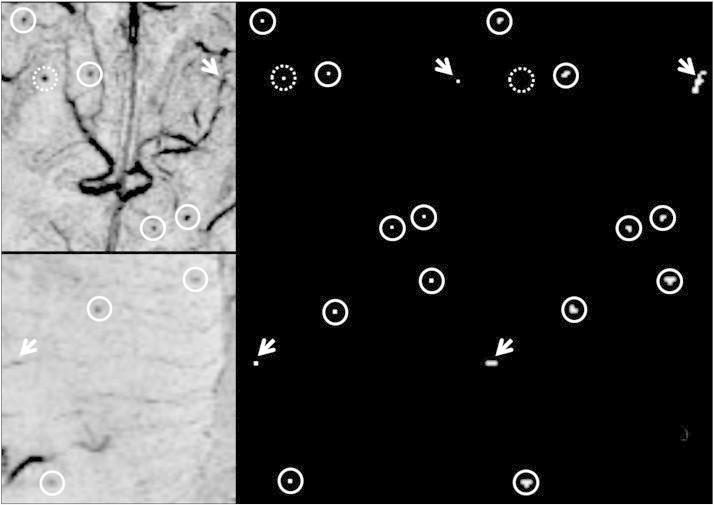
Representative examples of true CMBs detected by our algorithm. Top row: The center of 5 Definite CMBs (circles) and 1 false positive (arrow) from a vessel on mIP SWI image (left) are highlighted on the FRST map (middle). After 3D region growing and geometric feature examination, all true CMBs were identified and the false positive was eliminated because of the linear shape of its grown region (right). One true CMB (dashed circle) was directly identified because its |S| > 170, and thus did not undergo subsequent analysis. Bottom row: three possible CMBs of low image contrast were correctly identified and one false positive was eliminated after region growing and geometric feature examination.

Fig. 5.

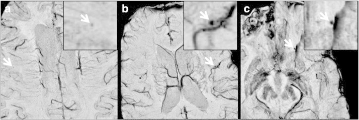
Typical false negatives found in our images. (a) A true possible CMB that was missed due to low contrast compared to surrounding tissue. (b) A missed true definite CMB that was removed by the vessel mask because of its proximity to a neighboring vessel. (c) A true definite CMB that was eliminated after geometrical feature examination due to region growing into susceptibility artifacts introduced by unsuccessful phase unwrapping during SWI processing.

The initial detection using the FRST identified 3162 potential CMB candidates, 90.8% of which were false positives. Only 1.0% of these false positives were produced after initial thresholding of the FRST maps with |S| > 170 and therefore did not undergo false positive reduction. The remaining false positives were generated after thresholding the FRST maps with lower thresholds. If the vessel mask had not been used, the number of false positives would have been 6 times as large. After region growing, 84.4% of these false positives were eliminated with a final average of 44.9 false CMBs identified per patient (range 23–65). The majority of these stemmed from tortuous, terminating, or transverse vessels and 17.4% (7.8/patient) were found in ventricles, tumor cavities and areas of susceptibility artifacts at air–tissue interfaces as demonstrated in Fig. 6.

Fig. 6.

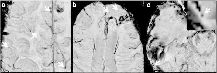
Typical false positives found in our experiments. (a) Four false positives (arrows) seen at the ending, cross section, or turning point of vessels. (b) Two false positives found in the tumor cavity. (c) A false positive presented in the susceptibility artifacts in the air–tissue interface.

The efficiency and performance of our algorithm compared to previously published methods are presented in Table 3. The computation time of the algorithm was approximately 1 min per patient using one core of a Linux workstation with Intel core 2 quad processors at 3.0 GHz and 8 GB of RAM. Our algorithm achieved the highest sensitivity with the lowest percentage of false positives per CMB and the fastest computation. Our results were also validated on a larger sample size both in terms of the total number of CMBs and the average number of CMBs per patient.

Table 3.

Comparison of efficiency among CMB detection algorithms.

Algorithm	Number of patients	True CMBs		Sensitivity	False positives			Computation time
		Total	Mean		Total	Per patient	Per CMB
Seghier et al.	30	114	3.8	50%	NAa	NA	NA	3 min (PC with 64-bit 3.2 GHz CPU, 12 GB RAM)
Barnes et al.	6	120	20	81.7%	645	107.5	5.4	1 minb
Kuijf et al.	18	66	3.7	71.2%	309	17.2	4.7	1 hc (One core of a standard workstation)
Bian et al.	10	304	30.4	86.5%	449	44.9	1.5	1 min (One core of a Linux workstation with quad processors at 3.0 GHz, 8 GB RAM)

^aThe information was not provided in the publication.

^bThe information of computation power was not specified in the publication.

^cThe time used for image segmentation and registration was not included.

4. Discussion

Development of computer-aided detection methods for CMBs is challenging because of their small size, wide distribution, and the presence of other structures that mimic their appearance. The need to identify radiation-induced CMBs with low contrast is a further factor that complicates their detection. Despite several previous attempts to address this problem, it remains a topic of active research. In this study, we have presented a semi-automated CMB detection algorithm that has achieved superior performance with a sensitivity of 86.5% and computation time of 1 min.

Achieving high sensitivity was the top priority in designing our algorithm because it has more impact than specificity on the performance that can be achieved. From a practical standpoint, visual inspection to remove false positive lesions is far easier than identifying CMBs missed by the detection algorithm, as the eye can more rapidly dismiss lesions falsely labeled as CMBs than it can search the entire imaging volume for true CMBs. The overall performance of our algorithm depended on both the size and contrast of CMBs, which is supported by the heightened sensitivity that was observed for definite CMBs compared to possible ones (95.4% vs. 77.5%). The newly formed radiation-induced CMBs that were evaluated in this study are typically harder to detect than CMBs caused by trauma or other mechanisms of disease, as they are often smaller in size and have varied contrast. Thus, we anticipate that our algorithm would be even more robust when applied to other patient populations.

The high sensitivity of our algorithm may be explained to the strength of our false positive reduction strategy. Screening of the FRST map by applying a vessel mask allowed the use of a much lower threshold for the FRST map and maximized sensitivity to smaller and low contrast CMBs during the initial detection step. This method facilitated the detection of 96.1% of all true CMBs, which included 100% of definite CMBs and missed a relatively small number of possible low-contrast CMBs. If this vessel mask had not been applied, it would have been necessary to use a higher threshold, which would have sacrificed the detection sensitivity. Although true CMBs can be masked if they are adjacent to the structures that are included, the number of these CMBs was small (2.0%; 1 definite and 5 possible) for our experiments.

Another significant contributor to our high sensitivity in initial detection was the 3D region growing process. Although a potential pitfall that is inherent for region growing is the occasional inclusion of neighboring pixels containing nearby vessels or susceptibility artifacts (Fig. 5c), we only applied region growing to a subset of CMBs with lower contrast and smaller size. Bypassing region growing for large CMB candidates afforded reduced thresholds for geometric features, which lead to more efficient false positive reduction. This separate processing pipeline for large and small CMBs resulted in the removal of only 7.6% (6 definite and 17 possible) of true CMBs during subsequent region growing.

Our method achieved a higher sensitivity, faster computation speed, and a reduced number of false positives compared with other related approaches. Also the performance of our algorithm was validated on a larger sample size in terms of total number of CMBs and incidence per patient (Table 3), demonstrating the robustness of our method. In particular there was heightened sensitivity (86.5% vs. 71.2%) compared to the other method based on FRST (Kuijf et al., 2012). Moreover, it should be noted that many of our CMBs spanned a smaller number of pixels than Kuijf et al. (2012) (average diameter: 2.08 vs. 2.28 pixels) and hence posed a greater challenge. This improved sensitivity applied even to the possible CMBs that had an average diameter of 1.84 pixels and after normalization had an average minimum intensity up to 26.8% of the maximum.

Unlike previously published studies, our elevated sensitivity is achieved without compromising computation speed. The fast computation of our algorithm originates from its simple design. Skull extraction and intensity normalization are the only preprocessing steps required, whereas other methods utilize image registration (Kuijf et al., 2012; Seghier et al., 2011) and/or segmentation (Kuijf et al., 2012) routines prior to applying their detection algorithms. In the initial detection step, gradient-based FRST can quickly locate local hypointense regions as potential CMBs. The computation time for FRST is further reduced in our algorithm by eliminating the convolution step originally proposed by Loy and Zelinsky (2003). In addition, the transform is repeatedly computed only at 3 radii in our experiments, while it was compute by Kuijf et al. at 18 radii. Finally, 3D region growing is performed within only a small local region for each candidate CMB, and only 3 geometrical features (area, circularity and centroid) are quantified to sequentially remove falsely identified CMBs, whereas the method of Barnes et al. (2011) utilizes 14 features associated with the shape, intensity, and size of CMBs in a support vector machine to perform the classification, which takes up to multiple days for parameter training.

3D region growing was implemented in our algorithm in order to reduce the number of false positives that were present after the FRST step. This allowed geometric features of a potential CMB to be extracted and was used in our study to eliminate 86.1% of false positives. The remaining false positives (1.5/CMB and 44.9/patient) originated mostly from vessels, susceptibility artifacts, or the surgical cavity. Overall, our algorithm produced a smaller percentage of false positives per true CMB than previous ones. Since radiation-induced CMBs are often smaller and of lower contrast, there is a trade-off between producing a small number of false positives and maintaining the high detection sensitivity achieved in our study. Kuijf et al. (2012) used gray/white matter masks to exclude brain structures such as ventricles and sulci, where false positives are often observed. The disadvantage of this approach is that it requires the acquisition of a T1-weighted image as well as the application of registration and segmentation algorithms that prolong the total processing time. In addition, all of our patients received intracranial tumor resection, which produces structures that mimic CMB (see Fig. 6b). These structures can be removed quickly during the final visual inspection because of their obvious anatomical location. A strict performance comparison of automated detection algorithms is difficult at this point, as the size and contrast of CMBs may vary with other experimental factors such as field strength and resolution (Nandigam et al., 2009). The manual review process and patient inclusion criteria are also all different among these studies. It is desirable in the future to construct a standard CMB database, in which CMBs are categorized by their disease type, MR imaging field strength, distribution or other related factors. This will not only help objectively evaluate automated CMB detection algorithms but also facilitate the training process for these algorithms.

The success of our algorithm demonstrates the advantage of a using a vessel mask to remove false positives in achieving a high sensitivity while maintaining a reasonable specificity in CMB detection. While methods that are able to create a high quality vessel mask in 3D using SWI have been proposed in literature (Koopmans et al., 2008), we used the vessel mask from the FRST transform in our approach because of its robustness and simplicity in integrating with our algorithm's pipeline. The better delineation and continuity of veins on mIP SWI compared to non-projected images facilitated both the generation of a more reliable vessel mask by FRST and a greater extent of region growing on these structures, both of which aided in reducing false positives. The improved false positive reduction can in turn be used to enhance detection sensitivity, e.g., set up a low threshold to screen the FRST map and make the initial detection highly sensitive. Limitations associated with the usage of mIP SWI images include susceptibility artifacts at air–tissue interfaces and magnified background noise that is introduced during reconstruction of SWI images that can be a potential source of false positives (Fig. 6c). Also the original location of CMBs cannot be determined on these images because of the projection processing, but it can easily be recovered on the original non-projected images. The projection processing may also accidentally project some CMBs in or close to certain dark structures that do not surround them in actual anatomy, leading to decreased FRST response or leakage in region growing, which both increase the number of false negatives. Despite these limitations, using FRST on mIP SWI images is especially advantageous for the detection of radiation-induced CMBs, whose essentially low contrast on conventional T2*-weighted magnitude images as the result of its small size is greatly improved on mIP SWI (Lupo et al., 2012). Furthermore, processing MR image using mIP has been suggested as a required step for visual CMB detection, especially when high resolution images acquired at high field strengths (e.g., 3 T or 7 T) are used (de Bresser et al., in press). As visual inspection (e.g., further false positive removal) of the output from automated CMB detection is still required, it is desirable to design an algorithm that operates on the same images that are used for subjective interpretation.

Finally, there are several limitations associated with our algorithm itself. First, while 3D region growing is a simple and fast method to segment putative CMBs, its capability to discriminate desired objects from close but dissimilar background is limited, making the segmentation leakage being more likely to happen for CMBs with low image contrast. To improve the accuracy of the segmentation, more advanced and finer techniques such as active contours and let sets may be used (Osher and Sethian, 1988), but at the expense of computation time. Second, at the very first and last image slices, the efficiency of geometric examination becomes lower due to limited space for region growing along slice selection direction. This may result in there being a higher number of false positives on these slices than on inner slices. Like previous published methods, training is an inevitable step that is required to apply our algorithm to detect CMBs from different types of diseases, different MR field strengths, and even different scan parameters such as TE, spatial resolution, and slice thickness. Size and contrast variation are the principal reasons that training is necessary, as most of parameters selected in our algorithm require that the range of CMB size and intensity be considered. However, the time used for training our algorithm is small as most of the parameters used in the algorithm can be empirically determined by studying a few representative CMBs as long as prior knowledge about the size of CMBs is available. Optimal values for other parameters such as MID and C can be determined empirically or formally by constructing ROC curves on a small training dataset such as we did in this study.

5. Conclusions

This study presented a method for semi-automated CMBs detection that uses mIP SWI, 2D FRST and 3D region growing. The FRST is used for initial lesion detection, and false positives are removed from putative CMBs identified in the first step using a region growing process with geometric feature examination. Our method achieved higher sensitivity with an acceptable number of false positives and faster computation time when compared to previously developed methods. Although it was evaluated for CMBs arising in the setting of prior radiation therapy for gliomas, its superior performance is likely to be of interest for detecting CMBs associated with other neurologic disorders, including CAA, hypertension, and TBI.

References

- Ayaz M., Boikov A.S., Haacke E.M., Kido D.K., Kirsch W.M. Imaging Cerebral Microbleeds Using Susceptibility Weighted Imaging: One Step Toward Detecting Vascular Dementia. Journal of Magnetic Resonance Imaging. 2010;31:142–148. doi: 10.1002/jmri.22001. [DOI] [PMC free article] [PubMed] [Google Scholar]
- Barnes S.R., Haacke E.M., Ayaz M., Boikov A.S., Kirsch W., Kido D. Semiautomated detection of cerebral microbleeds in magnetic resonance images. Magnetic Resonance Imaging. 2011;29:844–852. doi: 10.1016/j.mri.2011.02.028. [DOI] [PMC free article] [PubMed] [Google Scholar]
- Charidimou A., Werring D.J. Cerebral microbleeds: detection, mechanisms and clinical challenges. Future Neurology. 2011;6:587–611. [Google Scholar]
- Conijn M.M., Geerlings M.I., Biessels G.J., Takahara T., Witkamp T.D., Zwanenburg J.J., Luijten P.R., Hendrikse J. Cerebral microbleeds on MR imaging: comparison between 1.5 and 7 T. AJNR. American Journal of Neuroradiology. 2011;32:1043–1049. doi: 10.3174/ajnr.A2450. [DOI] [PMC free article] [PubMed] [Google Scholar]
- Cordonnier C., van der Flier W.M. Brain microbleeds and Alzheimer's disease: innocent observation or key player? Brain. 2011;134:335–344. doi: 10.1093/brain/awq321. [DOI] [PubMed] [Google Scholar]
- Cordonnier C., Al-Shahi Salman R., Wardlaw J. Spontaneous brain microbleeds: systematic review, subgroup analyses and standards for study design and reporting. Brain. 2007;130:1988–2003. doi: 10.1093/brain/awl387. [DOI] [PubMed] [Google Scholar]
- Cordonnier C., Potter G.M., Jackson C.A., Doubal F., Keir S., Sudlow C.L., Wardlaw J.M., Al-Shahi Salman R. improving interrater agreement about brain microbleeds: development of the Brain Observer MicroBleed Scale (BOMBS) Stroke. 2009;40:94–99. doi: 10.1161/STROKEAHA.108.526996. [DOI] [PubMed] [Google Scholar]
- de Bresser, J., Brundel, M., Conijn, M.M., van Dillen, J.J., Geerlings, M.I., Viergever, M.A., Luijten, P.R., Biessels, G.J., in press. Visual Cerebral Microbleed Detection on 7 T MR Imaging: Reliability and Effects of Image Processing. AJNR. American Journal of Neuroradiology. http://dx.doi.org/10.3174/ajnr.A2960. [DOI] [PMC free article] [PubMed]
- Fiehler J. Cerebral microbleeds: old leaks and new haemorrhages. International Journal of Stroke. 2006;1:122–130. doi: 10.1111/j.1747-4949.2006.00042.x. [DOI] [PubMed] [Google Scholar]
- Greenberg S.M., O'Donnell H.C., Schaefer P.W., Kraft E. MRI detection of new hemorrhages: potential marker of progression in cerebral amyloid angiopathy. Neurology. 1999;53:1135–1138. doi: 10.1212/wnl.53.5.1135. [DOI] [PubMed] [Google Scholar]
- Greenberg S.M., Vernooij M.W., Cordonnier C., Viswanathan A., Salman R.A.S., Warach S., Launer L.J., Van Buchem M.A., Breteler M.M.B., Grp M.S. Cerebral microbleeds: a guide to detection and interpretation. Lancet Neurology. 2009;8:165–174. doi: 10.1016/S1474-4422(09)70013-4. [DOI] [PMC free article] [PubMed] [Google Scholar]
- Gregoire S.M., Chaudhary U.J., Brown M.M., Yousry T.A., Kallis C., Jager H.R., Werring D.J. The Microbleed Anatomical Rating Scale (MARS): reliability of a tool to map brain microbleeds. Neurology. 2009;73:1759–1766. doi: 10.1212/WNL.0b013e3181c34a7d. [DOI] [PubMed] [Google Scholar]
- Haacke E.M., Xu Y.B., Cheng Y.C.N., Reichenbach J.R. Susceptibility weighted imaging (SWI) Magnetic Resonance in Medicine. 2004;52:612–618. doi: 10.1002/mrm.20198. [DOI] [PubMed] [Google Scholar]
- Koopmans P.J., Manniesing R., Niessen W.J., Viergever M.A., Barth M. MR venography of the human brain using susceptibility weighted imaging at very high field strength. Magma. 2008;21:149–158. doi: 10.1007/s10334-007-0101-3. [DOI] [PubMed] [Google Scholar]
- Kuijf H.J., de Bresser J., Geerlings M.I., Conijn M.M., Viergever M.A., Biessels G.J., Vincken K.L. Efficient detection of cerebral microbleeds on 7.0 T MR images using the radial symmetry transform. NeuroImage. 2012;59:2266–2273. doi: 10.1016/j.neuroimage.2011.09.061. [DOI] [PubMed] [Google Scholar]
- Loy G., Zelinsky A. Fast radial symmetry for detecting points of interest. IEEE Transactions on Pattern Analysis and Machine Intelligence. 2003;25:959–973. [Google Scholar]
- Lupo J.M., Banerjee S., Hammond K.E., Kelley D.A., Xu D., Chang S.M., Vigneron D.B., Majumdar S., Nelson S.J. GRAPPA-based susceptibility-weighted imaging of normal volunteers and patients with brain tumor at 7 T. Magnetic Resonance Imaging. 2009;27:480–488. doi: 10.1016/j.mri.2008.08.003. [DOI] [PMC free article] [PubMed] [Google Scholar]
- Lupo J.M., Chuang C.F., Chang S.M., Barani I.J., Jimenez B., Hess C.P., Nelson S.J. 7-Tesla susceptibility-weighted imaging to assess the effects of radiotherapy on normal-appearing brain in patients with glioma. International Journal of Radiation Oncology, Biology, and Physics. 2012;82:e493–e500. doi: 10.1016/j.ijrobp.2011.05.046. [DOI] [PMC free article] [PubMed] [Google Scholar]
- Nandigam R.N.K., Viswanathan A., Delgado P., Skehan M.E., Smith E.E., Rosand J., Greenberg S.M., Dickerson B.C. MR Imaging Detection of Cerebral Microbleeds: Effect of Susceptibility-Weighted Imaging, Section Thickness, and Field Strength. American Journal of Neuroradiology. 2009;30:338–343. doi: 10.3174/ajnr.A1355. [DOI] [PMC free article] [PubMed] [Google Scholar]
- Osher S., Sethian J.A. Fronts Propagating with Curvature-Dependent Speed - Algorithms Based on Hamilton-Jacobi Formulations. Journal of Computational Physics. 1988;79:12–49. [Google Scholar]
- Riccardi, A., 2006. A new computer aided system for the detection of nodules in lung CT exams. Ph.D. thesis, University of Bologna.
- Scheid R., Preul C., Gruber O., Wiggins C., von Cramon D.Y. Diffuse axonal injury associated with chronic traumatic brain injury: evidence from T2*-weighted gradient-echo imaging at 3 T. AJNR. American Journal of Neuroradiology. 2003;24:1049–1056. [PMC free article] [PubMed] [Google Scholar]
- Schenck J.F. The role of magnetic susceptibility in magnetic resonance imaging: MRI magnetic compatibility of the first and second kinds. Medical Physics. 1996;23:815–850. doi: 10.1118/1.597854. [DOI] [PubMed] [Google Scholar]
- Seghier M.L., Kolanko M.A., Leff A.P., Jager H.R., Gregoire S.M., Werring D.J. Microbleed detection using automated segmentation (MIDAS): a new method applicable to standard clinical MR images. PLoS One. 2011;6:e17547. doi: 10.1371/journal.pone.0017547. [DOI] [PMC free article] [PubMed] [Google Scholar]
- Smith S.M. Fast robust automated brain extraction. Human Brain Mapping. 2002;17:143–155. doi: 10.1002/hbm.10062. [DOI] [PMC free article] [PubMed] [Google Scholar]
- Vernooij M.W., van der Lugt A., Ikram M.A., Wielopolski P.A., Niessen W.J., Hofman A., Krestin G.P., Breteler M.M. Prevalence and risk factors of cerebral microbleeds: the Rotterdam Scan Study. Neurology. 2008;70:1208–1214. doi: 10.1212/01.wnl.0000307750.41970.d9. [DOI] [PubMed] [Google Scholar]
- Werring D.J., Coward L.J., Losseff N.A., Jager H.R., Brown M.M. Cerebral microbleeds are common in ischemic stroke but rare in TIA. Neurology. 2005;65:1914–1918. doi: 10.1212/01.wnl.0000188874.48592.f7. [DOI] [PubMed] [Google Scholar]