Towards real-time availability of 3-D temperature maps created with temporally constrained reconstruction

Abstract

Purpose

To extend the previously developed Temporally Constrained Reconstruction (TCR) algorithm to allow for real-time availability of 3D temperature maps capable of monitoring MR-guided high intensity focused ultrasound (MRgHIFU) applications.

Methods

A real-time TCR (RT-TCR) algorithm is developed that only uses current and previously acquired undersampled k-space data from a 3D segmented EPI pulse sequence, with the image reconstruction done in a GPU implementation to overcome computation burden. Simulated and experimental data sets of HIFU heating are used to evaluate the performance of the RT-TCR algorithm.

Results

The simulation studies demonstrate that the RT-TCR algorithm has sub-second reconstruction time and can accurately measure HIFU-induced temperature rises of 20 °C in 15 seconds for 3D volumes of 16 slices (RMSE = 0.1 °C), 24 slices (RMSE = 0.2 °C), and 32 slices (RMSE = 0.3 °C). Experimental results in ex vivo porcine muscle demonstrate that the RT-TCR approach can reconstruct temperature maps with 192 × 162 × 66 mm 3D volume coverage, 1.5 × 1.5 × 3.0 mm resolution, and 1.2 second scan time with an accuracy of +/− 0.5°C.

Conclusion

The RT-TCR algorithm offers an approach to obtaining large coverage 3D temperature maps in real-time for monitoring MRgHIFU treatments.

Introduction

Performing non-invasive thermal therapy procedures under the guidance of magnetic resonance imaging provides the ability to obtain real-time temperature measurements for monitoring and controlling the treatment (1–6). While many MRgHIFU applications have been successfully carried out with imaging that uses a multi-slice 2D approach (6–7), such monitoring has several drawbacks that leave room for improvement. Multi-slice 2D imaging cannot cover the entire ultrasound beam path, leaves gaps between slices, and cannot be interpolated to finer voxel spacing in the slice direction. For applications such as transcranial MR-guided high intensity focused ultrasound (MRgHIFU), optimal monitoring requires 3D temperature maps with large volume coverage and high spatio-temporal resolution in order to accurately track the rapid heating at the focus while simultaneously monitoring for heating that may occur at bone-tissue interfaces in the near- and far-fields of the ultrasound beam (8–10).

Extending MR temperature imaging to include large volume 3D coverage is a difficult problem as the tradeoff among spatial resolution, temporal resolution, and volume coverage is inherent in MRI. Investigators have used both single-shot and segmented echo-planar-imaging (EPI) (11–12) to rapidly acquire several slices distributed over the 3D volume of interest, for example in orthogonal planes through the HIFU focus (13) or divided between covering the focus and covering a region in the near-field (14). Another approach being investigated “sweeps” a 2D slice over the 3D volume of interest and incorporates predictions from a thermal model to generate 3D temperature maps (15–16). The approach of Mei et al. uses a truly 3D sequence combined with a reduced field-of-view (FOV) excitation and data undersampling with an UNFOLD reconstruction (17). Each approach improves upon the amount of coverage achieved, but none is able to fully monitor the entire 3D volume of interest.

Our group has previously published an approach to solving the problem of obtaining large coverage 3D temperature measurements, which we call temporally constrained reconstruction (TCR) (18–20). The method uses a 3D segmented EPI sequence that acquires undersampled data over the 3D volume of interest. The undersampled data is reconstructed with a compressed-sensing like approach that enforces data fidelity and constrains excessively rapid temporal changes. The method was shown to achieve accurate temperature measurements with 1.5 × 1.5 × 3.0 mm spatial resolution, 1.7 s temporal resolution, and 288 × 162 × 78 mm volume coverage (20). However, a major limitation to the approach as currently implemented is that it could not achieve real-time availability of the temperature images and was therefore limited to retrospective applications. This limitation stemmed from the fact that the reconstruction algorithm utilized the entire 4D k-space data set as input and employed an iterative gradient descent minimization approach that took several minutes to converge.

This work extends the TCR method to make real-time availability of the reconstructed temperature images possible. We refer to the updated algorithm as real-time TCR (RT-TCR). The RT-TCR algorithm only uses acquired k-space data up to the current time and takes advantage of GPU computing to obtain the reconstructed temperature maps within sub-second latency time. Simulation studies are performed to assess the accuracy of the RT-TCR method as a function of data acquisition volume relative to temperature rate of change, and also as a function of noise. Experimental HIFU studies are presented for cases of ex vivo porcine muscle heating and ex vivo transcranial applications.

Methods

Real-Time TCR Algorithm

The original TCR algorithm uses the entire 4-D data set to reconstruct images, m, from k-space data, d, by iteratively minimizing a cost function (20):

$$m=\text{arg}{\mathit{min}}_{m\prime }(\mid \mid \mathit{WF}(m\prime )-d\mid {\mid }_2^2+\alpha {\Sigma }_i^N\mid \mid {\nabla }_{t}m{\prime }_i\mid {\mid }_2^2)$$ [1]

where F( ) is the Fourier Transform, W is a binary function that represents which phase encoding lines have been acquired, m' is the image sequence estimate, α is a spatially varying free parameter, and the sum is over the N pixels in the image data set. The two terms in the cost function impose penalties on deviations from the acquired data and excessively rapidly changes in time, allowing convergence of the undersampled k-space data to an alias-free image. The cost function is minimized using a gradient descent algorithm with fixed step size and 100 iterations (18).

To achieve real-time availability of the temperature maps, the RT-TCR algorithm is modified and extended from the original TCR algorithm in three ways: 1) the computation time is reduced by a combination of implementing the code in a GPU environment and truncating the size of the data matrix in both space and time; 2) only information from current and past time frames are used as input to the cost function; 3) temperature information from several time frames of this reconstructed image data is used to create an estimate the temperature of the current time frame and also update the temperature estimation of previous time frames.

Graphics processing units (GPUs) have been widely used in medical imaging with successful applications covering image computing, visualization, and analysis (21–24). To implement the TCR algorithm in a GPU environment, it was rewritten from the original MATLAB™ (Mathworks, Inc.)-based version using open-source packages, namely CUFFT and CUBLAS in the CUDA software platform, and then wrapped to form MATLAB executable (mex) files. The GPU implementation was done on an NVIDIA Quadro 6000 with 448 cores. To further reduce the computation time, the data matrix passed to the algorithm is truncated in the x- and z-directions in image space (read-out and slice), such that only a small region around the HIFU focal zone is reconstructed using the RT-TCR algorithm. The remaining regions, where temperatures are either static or change significantly more slowly, are reconstructed with a sliding window approach. The data truncation is done by adding the most recently acquired k-space data to the previous k-space frames in a sliding window fashion, transforming to image space, truncating the x- and z-directions, and transforming back to k-space. Truncation is not done in the y-direction because the undersampling is done in the phase-encode direction.

The RT-TCR algorithm reconstructs the current time frame based only on current and past information, but also updates that time frame as “future” information becomes available. The first step to reconstructing the current time frame, t, is to use the acquired k-space data from frames t-P through t as input for the cost function of Equation 1, where P is twice the reduction factor (P = 12 throughout this work). With this subset of data, the TCR algorithm is run in its original form to create an estimate of the complex images for time frames t-P to t. Because the TCR algorithm relies on temporal gradient information, it is known that the image estimates for the most recent time frames will be sub-optimal, with a bias towards underestimating the extent of the temporal changes that are occurring.

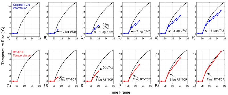
The remaining steps of the RT-TCR algorithm are designed to create temperature maps that partially overcome this underestimation bias. An example reconstruction of simulated data is shown in Figure 1 where the dashed black line shows the true temperature, the blue lines in the top row show the temperature information obtained from the original TCR algorithm, and the red lines in the bottom row show how that information is combined to obtain the RT-TCR temperatures. The uppermost blue dots in the top row represent the temperatures that would be calculated if only the original TCR algorithm were used with present and past data. It can be seen that these underestimate the true temperature changes. The blue connecting lines represent the temperature temporal derivatives that are calculated to reconstruct the RT-TCR temperatures. Consider the reconstruction of time frame 22 (Figure 1C and 1I) where k-space data from frames 10 through 22 are used in the original TCR algorithm to create the complex image data and TCR temperatures. Four pieces of TCR temperature information are used to create the RT-TCR temperature estimate: the current TCR estimate of the temperature at frame 22 (T = 3.05°C) and the previous TCR estimate of the temperature at frame 21 (T = 1.45°C) are used to calculate the most recent temperature derivative (0 lag dT/dt); similarly, the current TCR estimate of the temperature at frame 21 (T = 2.10°C) and the previous TCR estimate of the temperature at frame 20 (T = 0.0°C) are used to calculate the next most recent temperature derivative (1 lag dT/dt). The RT-TCR estimate of the temperature for the current frame 22 is created by summing these temperature derivatives (T_RT-TCR = 1.6°C + 2.1°C = 3.7°C), and the updated RT-TCR estimate of the temperature for the past time frame 21 is also created by summing the appropriate temperature derivatives (T_RT-TCR = 2.1°C).

Figure 1.

Explanation of the RT-TCR algorithm. Simulated temperature vs time plots shown, with the true temperature in dashed black, temperature and temperature temporal derivative information obtained from the original TCR algorithm shown in blue on the top row, and the RT-TCR temperatures shown in red on the bottom row. The RT-TCR temperatures are calculated using the dT/dt information from the original TCR algorithm and are updated as new information comes in.

The process continues to reconstruct frames 23 and beyond, where the RT-TCR temperature estimate is always a summation of the temperature temporal derivative terms calculated from the original TCR algorithm. Only information from the five previous time frames is used in the RT-TCR estimation as older information from the sixth previous time frame and before contributes negligibly. The final RT-TCR temperatures are therefore obtained after a 5-time frame lag. The plots in Figure 1H–L show how the RT-TCR algorithm is able to provide a good estimate of the current temperature in real-time, and also how the temperature estimates of previous time frames are updated as new information comes in until they are as good as would be obtained from using the entire 4D data set in the original TCR algorithm.

For the original TCR algorithm to reconstruct a data set with 192 × 108 × 30 image matrix and all 77 time frames, it took 236 seconds on a 12-core computer with Dual Intel Xeon Processor X5650, 2.66Ghz processing speed, and 64 GB of RAM. For the RT-TCR to reconstruct one time frame from this set, it was truncated to an image matrix size of 10 × 108 × 13, used the 13 most recent time frames and took 0.25 seconds with the GPU implementation on an NVIDIA Quadro 6000 with 448 cores running at 574 MHz, and 6 GB of RAM on the GPU. It took 0.35 seconds to transfer the data from the scanner computer to the GPU machine, 0.02 seconds to do the necessary pre-processing steps, and 0.10 seconds for the post-processing. The total reconstruction time of 0.72 seconds is less than the data acquisition time for one undersampled time frame in the examples presented here.

Simulation Studies

Simulation data sets were created to mimic undersampled k-space data from a 3D segmented EPI acquisition. 4D temperature distributions were simulated at 0.5 mm isotropic spatial resolution and 30 ms temporal resolution using the beam intensity pattern from a phased array HIFU transducer (described below) and the Pennes Bioheat Equation (25) (thermal properties assumed to be density = 1,000 kg/m³, specific heat = 3,800 J/kg/°C, thermal conductivity = 0.5 W/m/°C, perfusion = 0 kg/m³/s, maximum specific absorption rate = 6.7×10⁵ W/m³). These original temperatures were considered truth for all simulation studies. To test the RT-TCR algorithm, the simulated temperatures were converted into k-space data using the standard proton resonance frequency (PRF) shift relation between temperature and phase (26–27) and a constant image magnitude. This fully sampled k-space data was truncated in frequency space to downsample the spatial resolution to 1.0 × 1.0 × 3.0 mm. The data was then sampled using a 3D segmented EPI approach, as described in the earlier TCR paper (20). For every 30 ms time step, 9 lines of k-space were sampled from the current time frame into the undersampled k-space data matrix. This was repeated until all k-z phase encodes had two echo trains of data each, giving one undersampled time frame. For example, a 16-slice 3D volume with 108 k-y phase encodes and an EPI factor of 9 would receive 288 total kx lines over a time span of 0.96 seconds, spread evenly in the k-y direction and fully sampled in the k-x and k-z directions, for a data reduction factor of 6. The simulated image parameters were: 1.0 × 1.0 × 3.0 mm resolution; 128 × 108 × Z imaging matrix (where Z = 16, 24, and 32 slices); TR = 30 ms; TE = 10 ms; EPI Factor = 9; 6× undersampling; 0.96, 1.44, and 1.92 seconds per undersampled time frame for the 16, 24, and 32 slice volumes.

The first simulation study was designed to assess the performance of the RT-TCR algorithm as a function of achievable volume coverage relative to the HIFU-induced temperature rate of change. Data sets were simulated to achieve a 20°C temperature rise over 60 seconds, 30 seconds, and 15 seconds, which corresponded to temperature rates of change of 1.7 °C/s, 2.1 °C/s, and 2.8 °C/s at the onset of heating. Undersampled k-space data sets created from these temperatures were reconstructed using the RT-TCR algorithm for 16-slice, 24-slice and 32-slice volumes. The metrics used to evaluate the RT-TCR performance were temperature root mean square error (RMSE) over all voxels experiencing greater than 2°C temperature rise and maximum temperature at the conclusion of heating. For comparison, these metrics were also calculated for a basic sliding window reconstruction of the data.

The second simulation study was designed to assess the performance of the RT-TCR algorithm as a function of noise. The 24-slice, 20°C temperature rise in 30 seconds data set was used. Zero-mean Gaussian random noise was added to the undersampled k-space data at increasing levels, with different realizations of the same noise level added to the real and imaginary parts of k-space. Five noise levels were chosen such that a sliding window reconstruction of the noisy k-space data produced temperature maps with temperature standard deviations of 0.25°C, 0.5°C, 1.0°C, 1.5°C, and 2.0°C, as measured over an ROI consisting of a 5×11×5 region of unheated voxels and all time frames. The noisy k-space data was reconstructed with the RT-TCR algorithm and a standard sliding window reconstruction, with noise generation and reconstruction repeated 25 times for each noise level. The same metrics of temperature RMSE and maximum temperature were used for evaluation.

Experiments

All HIFU heating experiments were carried out in a Siemens TIM Trio MRI scanner (Siemens Medical Solutions, Erlangen, Germany) using an MRI-compatible phased array transducer (256 elements, 1 MHz frequency, 13 cm radius of curvature, Imasonic, Besancon, France and Image Guided Therapy, Pessac, France). Imaging for all experiments was done with a 3D segmented EPI gradient echo sequence, with even undersampling done as described in the previous paper (20).

In the first set of experiments, HIFU heating was done on an ex vivo pork muscle sample at three different sonication power and duration combinations: 18 acoustic watts for 60 seconds, 36 W for 30 seconds, and 72 W for 15 seconds. The temperature rates of change at the onset of heating for these powers were 1.1 °C /s, 2.2 °C /s, and 3.1 °C /s. For each power level, the heating was repeated twice under identical circumstances. In the first instance, imaging parameters were chosen such that the 3D volume could be fully sampled at adequate temporal resolution. These fully sampled data sets were reconstructed with the standard Fourier Transform approach and used to compute temperature maps that were considered to be truth. In the second instance, larger 3D volumes were acquired at an undersampling factor of 6× and reconstructed with the RT-TCR algorithm. Each pair of identical heating runs was performed at the same location in the sample. To avoid tissue damage in the sample, the focal zone was translated by approximately 1 cm in between the three pairs of runs and the starting temperature of the sample (~15°C) was low enough such that negligible thermal dose accrued during HIFU heating. The metrics used to evaluate the RT-TCR temperatures were temperature RMSE over all voxels experiencing greater than 2°C temperature rise and maximum temperature at the conclusion of heating. The same metrics for a sliding window reconstruction of the undersampled data were also calculated for comparison. Imaging parameters for the fully sampled data were: 1.5 × 1.5 × 3.0 mm resolution, 128 × 72 × 12 imaging matrix (10 slices plus 20% slice oversampling), TR = 25 ms, TE = 10 ms, EPI Factor = 9, flip angle = 20°, bandwidth = 738 Hz/pixel, 2.4 seconds per scan. Imaging parameters for the undersampled data were: 1.5 × 1.5 × 3.0 mm resolution, 128 × 108 × 24 imaging matrix (22 slices plus 9% slice oversampling), TR = 25 ms, TE = 10 ms, EPI Factor = 9, flip angle = 20°, bandwidth = 738 Hz/pixel, 6× undersampling, 1.2 seconds per undersampled time frame.

The second HIFU heating experiment was done to demonstrate the utility of the RT-TCR method for monitoring transcranial MRgHIFU procedures. A plastic replica of a human skull was embedded in an agar mold, with the HIFU focus targeted 6.5 cm into the phantom from the skull surface. Phase aberration correction of the ultrasound beam was not performed. Two 3D imaging slabs were acquired simultaneously in interleaved fashion, one covering the focal zone and one covering the region where the near-field of the ultrasound beam path intersected the skull surface in order to capture any heating that may occur at the inner skull/agar interface. The temperatures at the focal zone are expected to rise rapidly, and therefore these were reconstructed with the RT-TCR algorithm. However, temperature changes on the skull surface were expected to occur much more slowly and therefore a sliding window reconstruction was used and assumed to be adequate for capturing these changes. The imaging parameters were: 1.5 × 2.0 × 2.5 mm resolution, 192 × 121 × 32 imaging matrix (14 slices per slab plus 14% slice oversampling for each slab), TR = 30 ms, TE = 12 ms, EPI Factor = 11, flip angle = 15°, bandwidth = 744 Hz/pixel, 5.5× undersampling, 1.9 seconds per undersampled time frame.

Results

Simulation

Temperature versus time plots are shown in Figure 2 for the nine different data sets simulated at different ultrasound powers, heating durations and imaging volumes. Truth is shown in black, the RT-TCR temperatures that would be obtained without any lag time in red, and the final RT-TCR temperatures in green. Note that the plots for “RT-TCR, 0 lag” show for each time step the temperatures that would be reconstructed in real-time and that any “past” time frames have not been updated. Similarly, the plots for “RT-TCR, Final” show for all time steps the final RT-TCR temperatures after all updating has been done. The RT-TCR temperatures obtained in real-time cannot quite follow the abrupt changes in temperature when the heating is turned on and off, even when the time of ultrasound switching on/off is known a priori. As expected, this lagging behavior increases with both volume coverage and the true temperature rate of change. For slower rates of change or less volume coverage, the RT-TCR temperatures with 0 lag are able to follow truth reasonably well, and the final RT-TCR temperatures are able to match truth well for all cases.

Figure 2.

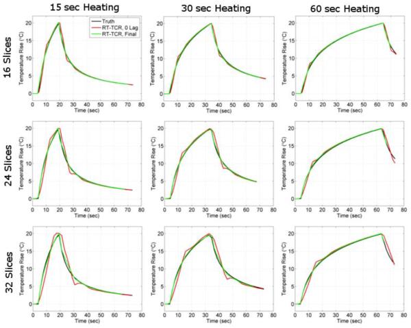
Simulation results showing temperature versus time plots for the voxel in the center of the HIFU focal zone. Three heating rates (20°C rise in 15, 30, and 60 seconds) and three data volume sizes (16, 24, and 32 slices) were considered. The true simulated temperatures are plotted in black; the temperatures obtained from the RT-TCR algorithm without any lag in red; and the final temperatures obtained from the RT-TCR algorithm in green.

More simulation results from the three 24-slice data sets are shown in Figure 3. The first column shows the true temperature maps at peak heating for each heating duration. The next two columns show temperature differences over all time frames for a vertical line of data through the center of the focal zone (as noted by the dashed yellow line). The dashed black lines represent times that the ultrasound is being turned on and off. It can be seen that the RT-TCR temperatures will slightly underestimate the true temperature at the onset of heating and slightly overestimate it after the conclusion of heating. These are the times when the temperature gradient in time is changing the most rapidly.

Figure 3.

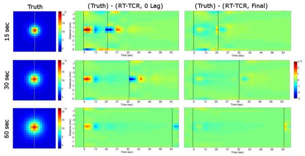
Left column: True temperature maps from 24-slice simulated data sets. Middle Column: Temperature difference between the true temperatures and RT-TCR temperatures with 0 lag for a line of voxels through the hotspot over time. Right column: Temperature difference between the true temperatures and final RT-TCR temperatures for the same line over time. Dashed black lines indicate ultrasound on/off.

A summary of the RMSE and maximum temperature metrics are presented in Table 1 for all nine simulated cases.

Table 1.

Root mean square error and the maximum temperature from all nine simulated data sets reconstructed with the RT-TCR algorithm and a basic sliding window approach.

	16 Slices			24 Slices			32 Slices
	15 s	30 s	60 s	15 s	30s	60 s	15 s	30 s	60 s
RMSE (°C)
RT-TCR, 0 Lag	0.1	0.1	0.1	0.2	0.1	0.1	0.3	0.2	0.2
RT-TCR, Final	0.1	0.1	0.1	0.1	0.1	0.1	0.1	0.1	0.1
Sliding Window	0.5	0.3	0.3	0.7	0.5	0.4	0.9	0.6	0.5
Max Temp (°C)
Truth	19.8	20.0	20.0	19.6	19.7	19.9	19.6	19.7	19.9
RT-TCR, 0 Lag	20.1	19.9	20.0	20.0	19.9	20.0	20.1	20.0	20.0
RT-TCR, Final	20.1	19.9	20.0	20.0	19.6	20.0	20.1	19.5	20.0
Sliding Window	18.2	19.4	19.7	17.1	18.7	19.5	16.3	18.3	19.4

The results from the simulation noise study are shown in Figure 4 and Table 2. Figure 4 shows temperature maps at the peak of heating from the 24-slice, 30-second heating data set. The true temperatures are shown in the first row, RT-TCR temperatures with 0 lag time shown in the second row, and the final RT-TCR temperatures shown in the third row. Increasing amounts of added noise are shown in the columns. The RMSE and maximum temperature results are summarized in Table 2. The RT-TCR algorithm does cause some amplification of noise. The RMSE values for the RT-TCR data with 0 lag are slightly more than double the RMSE values when random noise was added to the true temperatures. For the final RT-TCR temperatures, the RMSE values are approximately 40% greater than the RMSE values from the noisy true temperatures. Note that the noisier temperatures at the top and bottom of these RT-TCR temperature regions are from edge effects due to the truncated data set that is passed to the RT-TCR algorithm (only 20 pixels in the read-out direction). An appropriate level of data truncation would have to be chosen to avoid these noise effects contaminating important regions.

Figure 4.

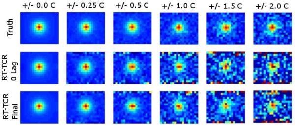
Simulation results showing temperature maps of peak heating for the 30- second heating, 24-slice data set with varying levels of noise added. Zero-mean Gaussian noise was added to achieve temperature standard deviations of 0.25°C, 0.5°C, 1.0°C, 1.5°C, and 2.0°C in a non-heated region. Maps are shown for the original simulated temperatures, the temperatures obtained from the RT-TCR algorithm without any lag, and the final temperatures obtained from the RT-TCR algorithm.

Table 2.

24-slice, 30 second heating simulated data set with five levels of noise added. 25 reconstructions performed at each noise level, with the mean and standard deviation reported for RMSE and maximum temperature.

	Noise Level
	0.25 °C	0.50 °C	1.00 °C	1.50 °C	2.00 °C
RMSE (°C)
Truth + Noise	0.3 +/− 0.0	0.5 +/− 0.0	1.0 +/− 0.0	1.5 +/− 0.0	2.0 +/− 0.0
RT-TCR, 0 Lag	0.6 +/− 0.0	1.1 +/− 0.0	2.3 +/− 0.0	3.4 +/− 0.0	4.6 +/− 0.0
RT-TCR, Final	0.3 +/− 0.0	0.7 +/− 0.0	1.4 +/− 0.0	2.1 +/− 0.0	2.8 +/− 0.1
Sliding Window	0.6 +/− 0.0	0.9 +/− 0.0	1.6 +/− 0.0	2.3 +/− 0.0	3.1 +/− 0.1
Temp STD (°C)
Sliding Window	0.3 +/− 0.0	0.5 +/− 0.0	1.0 +/− 0.0	1.5 +/− 0.0	2.0 +/− 0.0
RT-TCR, 0 Lag	0.5 +/− 0.0	0.9 +/− 0.0	1.9 +/− 0.0	2.8 +/− 0.0	3.8 +/− 0.0
RT-TCR, Final	0.2 +/− 0.0	0.4 +/− 0.0	0.9 +/− 0.0	1.3 +/− 0.0	1.7 +/− 0.0
Max Temp (°C)
Truth	19.7	19.7	19.7	19.7	19.7
Truth + Noise	19.8 +/− 0.3	19.6 +/− 0.5	19.6 +/− 1.2	19.2 +/− 1.4	19.5 +/− 2.1
RT-TCR, 0 Lag	20.1 +/− 0.5	19.9 +/− 0.8	19.5 +/− 2.1	20.0 +/− 3.5	19.3 +/− 4.3
RT-TCR, Final	19.8 +/− 0.4	19.5 +/− 1.2	19.0 +/− 1.2	20.1 +/− 2.4	19.3 +/− 4.3
Sliding Window	18.9 +/− 0.3	18.8 +/− 0.8	18.5 +/− 1.5	19.3 +/− 2.1	18.0 +/− 3.1

Experiment

Temperature versus time plots from the three ex vivo pork muscle HIFU heating experiments are shown in Figure 5. Fully sampled temperature data acquired with only 12 slices and a 2.4 second time step are considered to be truth and are shown in black. The 24-slice data acquired with k-space undersampling and reconstructed with the RT-TCR algorithm are shown in red for the RT-TCR temperatures with 0 lag and in green for the final RT-TCR temperatures. The RMSE and maximum temperatures are summarized in Table 3 for all three heating runs. As with the simulated data results, the 0 lag RT-TCR temperatures at the center of the focal zone cannot quite follow the most abrupt changes in temperature when the ultrasound is turned on and off, but are able to match the true temperatures when they are changing less rapidly. This lagging behavior can especially be seen right after the ultrasound is turned on in the 36 W and 72 W cases for the 0 Lag RT-TCR temperatures. When the entire focal zone is considered, the RT-TCR temperatures follow the fully sampled temperatures closely for all three heating cases, with the RMSE remaining below 1°C for both the RT-TCR temperatures with 0 lag and the final RT-TCR temperatures. Figure 6 shows coronal and transverse views through the 3D temperature volumes for the 36 W heating case at the peak of heating.

Figure 5.

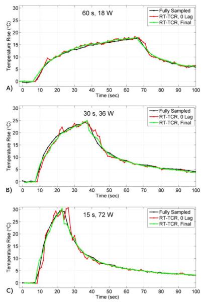
Experimental results from the ex vivo pork muscle HIFU heating showing temperature versus time plots for the voxel at the center of the focus. Fully sampled temperatures shown in black, RT-TCR temperatures with 0 lag in red, and final RT-TCR temperatures in green.

Table 3.

Ex vivo pork muscle experimental data. Root mean square error and the maximum temperature for all three data sets reconstructed with the RT-TCR algorithm and a basic sliding window approach.

	15 s, 72 W	30 s, 36 W	60 s, 18 W
RMSE (°C)
RT-TCR, 0 Lag	0.5	0.4	0.7
RT-TCR, Final	0.4	0.4	0.5
Sliding Window	0.8	0.5	0.6
Max Temp (°C)
Fully sampled	29.2	24.3	17.4
RT-TCR, 0 Lag	27.2	24.2	18.0
RT-TCR, Final	28.2	24.5	18.0
Sliding Window	24.6	23.3	17.6

Figure 6.

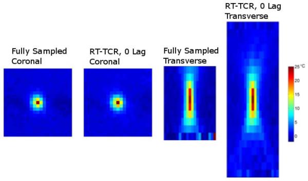
Temperature maps of the 36-watt, 30-second experimental HIFU heating in ex vivo pork muscle. Coronal and transverse slices through the 3D temperature volumes of the 10-slice fully sampled temperatures and the 22-slice undersampled temperatures reconstructed with the RT-TCR algorithm (0 lag).

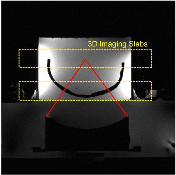
A transverse view of the experimental set up for the second HIFU heating experiment is shown in Figure 7. The two imaging slabs are oriented in the coronal direction, one to cover heating at the ultrasound focus and one to cover heating that may occur at the skull/agar interface. Temperature maps from the peak of heating are shown in Figure 8. The left images show three orthogonal views through the 3D volume slab covering the ultrasound focus, where the HIFU hotspot can be seen. This data was reconstructed with the RT-TCR algorithm and the final RT-TCR temperatures are shown. The right image is a 2D projection of the temperature rise measured on the inner surface of the skull/agar interface using information from the lower 3D imaging slab. The segmentation for the projection image included voxels from the agar that were directly adjacent to the skull in order to display the region with the most heating, however temperature rises due to heat diffusion extend a few millimeters from the skull surface. The circular pattern of the temperature rise indicates where the conical ultrasound beam path intersects the skull surface. Note that the temperature scales are different for the two images.

Figure 7.

Transverse view of the experimental set up for the through-skull HIFU heating experiment. A plastic human skull model is embedded in an agar phantom with the HIFU focus 6.5 cm deep into the skull. Two 3D imaging slabs are positioned to monitor the temperature rise at the focus and at the skull/agar interface.

Figure 8.

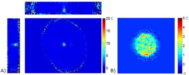
A) Three orthogonal views through the 3D temperature map volume covering the ultrasound focus. Temperatures reconstructed with the RT-TCR algorithm (Final RT TCR temperatures shown). B) 2D projection of the heating measured on the inner surface of the skull/agar interface. Temperature maps reconstructed with a basic sliding window approach.

Discussion

This work is aimed at solving the problem of attaining large coverage temperature maps with the spatial and temporal resolution necessary for accurate real-time monitoring of MRgHIFU procedures. We have taken the approach of using a 3D segmented EPI pulse sequence, combined with k-space data undersampling and a constrained reconstruction algorithm. In a previously published paper, this approach was shown to be successful when the entire 4D k-space data set was available as input to the TCR reconstruction algorithm. However, in order to be clinically useful, the temperature information must be available in real-time. This current manuscript describes an approach to extending the TCR approach to a real-time TCR implementation where the problems of reconstruction computation time and use of only current and past k-space data are overcome. The RT-TCR algorithm was tested with both simulated and experimental data. Experimental results demonstrate that the RT-TCR approach can reconstruct temperature maps with 192 × 162 × 66 mm contiguous 3D volume coverage, 1.5 × 1.5 × 3.0 mm resolution, and 1.2 second scan time with an accuracy of approximately +/− 0.5°C.

The first step in achieving real-time availability of the temperature maps was reducing the computation time of the iterative TCR algorithm. This was done by reducing the amount of data passed to the algorithm as input and implementing the code in a GPU framework. The reduction in the amount of spatio-temporal data passed to the TCR algorithm accounted for the majority of the computation time savings. However, data reduction by itself was not sufficient and the GPU implementation provided the necessary additional time savings. With the systems used in this work, the GPU version provided approximately a 3.5× speed up over the conventional CPU implementation for the same amount of data. The combination of data reduction and GPU implementation allowed the RT-TCR to produce the temperature maps in 0.72 seconds, a time that includes data transfer, the running of the original TCR algorithm with 100 iterations, and the RT-TCR algorithm pre- and post-processing steps. While not as fast as simply doing a traditional Fourier Transform reconstruction, this lag time is less than one acquisition step and should be adequate for most monitoring and temperature-based feedback needs. As computing power increases, this processing time will reduce even further.

The second component of the extension to achieve real-time temperature availability was to adapt the TCR algorithm such that only information up to the currently acquired k-space time frame was used in the reconstruction. The TCR algorithm employs a constraint in the temporal direction and therefore uses a second derivative in time in the minimization process. This temporal second derivative is best estimated when “future” data is available. Therefore, for a data series consisting of, for example, 13 time frames, the TCR reconstruction of the 7^th frame will be very good, but the reconstruction of the 13^th frame will not be as good. The RT-TCR algorithm improves the current temperature estimate, which is known to be sub-optimal, by using information from the previous frames, which are known to be better estimates of truth. The RT-TCR algorithm also updates the temperature history as new information comes in, such that the final RT-TCR temperatures will be equivalent to the original TCR algorithm that uses all information from the entire 4D data set.

One drawback to the RT-TCR algorithm is that this approach of using “past” temperature information to improve the estimate of the current time frame compounds errors due to noise. As currently implemented, the RT-TCR algorithm uses information from the 5 previous time frames to improve the estimate of the current time frame. The combination of 5 equally noisy temperature maps would be expected to result in a $\sqrt{5}\mathrm{X}$ increase in noise error. This is somewhat mitigated by the fact that the temporal constraint in the TCR algorithm acts to smooth random noise in time. For example, when noise was added to the simulated data at a level that produced a 1°C temperature STD in sliding window-reconstructed temperatures, the temperature STD for the RT-TCR temperatures with 0 lag averaged 1.9°C, and the final RT-TCR temperatures had a temperature STD of 0.9°C. For all noise levels, the temperature STD of the final RT-TCR temperatures was less than that of the sliding window temperatures.

Another limitation of the RT-TCR algorithm, and the TCR approach in general, is that it cannot handle situations where movement is occurring inside the field of view. The temporal constraint assumes that the object being imaged is fixed in time and motion will lead to reconstruction artifacts. Note, however, that motion outside of the field of view can be handled, even when it leads to susceptibility changes that affect the phase of the object inside the field of view (28). In these cases, a reference-less temperature calculation technique would be required as part of the RT-TCR algorithm in place of the standard phase subtraction approach (29). There are several MRgHIFU applications where motion of the anatomy inside the FOV is not a substantial problem, including ablation procedures in the breast and brain.

Despite these limitations, the RT-TCR approach to monitoring temperature changes during MR-guided thermal therapies offers a significant advantage over the fully sampled, multi-slice 2D imaging that is currently used in most applications. The advantage is greatly increased volume coverage without sacrificing spatial or temporal resolution. The contiguous 3D volume coverage can be used to monitor the entire focal zone and much of the near- or far-field of the beam path. The 3D volume could also be broken up to monitor two different regions of interest, as in the case of the trans-skull HIFU heating example. Because the sequence is truly 3D, zero-filled interpolation can be done in all three dimensions to create arbitrarily small voxel spacing and reduce partial volume effects. Simultaneous 3D monitoring of the focal zone and of regions outside of the ultrasound focus can be critical to avoiding inadvertent heating that may damage vital tissues.

References

- 1.Hynynen K, Damianou CA, Colucci V, Unger E, Cline HH, Jolesz FA. MR monitoring of focused ultrasonic surgery of renal cortex: experimental and simulation studies. J Magn Reson Imaging. 1995;5(3):259–266. doi: 10.1002/jmri.1880050306. [DOI] [PubMed] [Google Scholar]
- 2.Jolesz FA. Interventional magnetic resonance imaging, computed tomography, and ultrasound. Acad Radiol. 1995;2(Suppl 2):S124–125. doi: 10.1016/s1076-6332(12)80051-1. [DOI] [PubMed] [Google Scholar]
- 3.Mougenot C, Quesson B, de Senneville BD, de Oliveira PL, Sprinkhuizen S, Palussiere J, Grenier N, Moonen CT. Three-dimensional spatial and temporal temperature control with MR thermometry-guided focused ultrasound (MRgHIFU) Magn Reson Med. 2009;61(3):603–614. doi: 10.1002/mrm.21887. [DOI] [PubMed] [Google Scholar]
- 4.Salomir R, Palussiere J, Vimeux FC, de Zwart JA, Quesson B, Gauchet M, Lelong P, Pergrale J, Grenier N, Moonen CT. Local hyperthermia with MR-guided focused ultrasound: spiral trajectory of the focal point optimized for temperature uniformity in the target region. J Magn Reson Imaging. 2000;12(4):571–583. doi: 10.1002/1522-2586(200010)12:4<571::aid-jmri9>3.0.co;2-2. [DOI] [PubMed] [Google Scholar]
- 5.Zhang B, Yang X, Yang F, Qin C, Han D, Ma X, Liu K, Tian J. The CUBLAS and CULA based GPU acceleration of adaptive finite element framework for bioluminescence tomography. Opt Express. 2010;18(19):20201–20214. doi: 10.1364/OE.18.020201. [DOI] [PubMed] [Google Scholar]
- 6.McDannold N, Clement GT, Black P, Jolesz F, Hynynen K. Transcranial magnetic resonance imaging- guided focused ultrasound surgery of brain tumors: initial findings in 3 patients. Neurosurgery. 2010;66(2):323–332. doi: 10.1227/01.NEU.0000360379.95800.2F. discussion 332. [DOI] [PMC free article] [PubMed] [Google Scholar]
- 7.Chopra R, Tang K, Burtnyk M, Boyes A, Sugar L, Appu S, Klotz L, Bronskill M. Analysis of the spatial and temporal accuracy of heating in the prostate gland using transurethral ultrasound therapy and active MR temperature feedback. Phys Med Biol. 2009;54(9):2615–2633. doi: 10.1088/0031-9155/54/9/002. [DOI] [PubMed] [Google Scholar]
- 8.Huang Y, Song J, Hynynen K. MRI Monitoring of Skull-Base Heating in Transcranial Focused Ultrasound Ablation. Sweden; Stockholm: 2010. [Google Scholar]
- 9.Mougenot C, Kohler MO, Enholm J, Quesson B, Moonen C. Quantification of near-field heating during volumetric MR-HIFU ablation. Med Phys. 2011;38(1):272–282. doi: 10.1118/1.3518083. [DOI] [PubMed] [Google Scholar]
- 10.Payne A, Vyas U, Todd N, de Bever J, Christensen DA, Parker DL. The effect of electronically steering a phased array ultrasound transducer on near-field tissue heating. Med Phys. 2011;38(9):4971–4981. doi: 10.1118/1.3618729. [DOI] [PMC free article] [PubMed] [Google Scholar]
- 11.Kickhefel A, Roland J, Weiss C, Schick F. Accuracy of real-time MR temperature mapping in the brain: a comparison of fast sequences. Phys Med. 2010;26(4):192–201. doi: 10.1016/j.ejmp.2009.11.006. [DOI] [PubMed] [Google Scholar]
- 12.Salomir R, Rata M, Lafon C, Cotton F, Delemazure AS, Palussiere J, Chapelon JY. Automatic feedback control of the temperature for MRI-guided therapeutic ultrasound. Conf Proc IEEE Eng Med Biol Soc. 2007;2007:222–225. doi: 10.1109/IEMBS.2007.4352263. [DOI] [PubMed] [Google Scholar]
- 13.Enholm JK, Kohler MO, Quesson B, Mougenot C, Moonen CT, Sokka SD. Improved volumetric MR-HIFU ablation by robust binary feedback control. IEEE Trans Biomed Eng. 2010;57(1):103–113. doi: 10.1109/TBME.2009.2034636. [DOI] [PubMed] [Google Scholar]
- 14.Kohler MO, Mougenot C, Quesson B, Enholm J, Le Bail B, Laurent C, Moonen CT, Ehnholm GJ. Volumetric HIFU ablation under 3D guidance of rapid MRI thermometry. Med Phys. 2009;36(8):3521–3535. doi: 10.1118/1.3152112. [DOI] [PubMed] [Google Scholar]
- 15.Hey S, De Senneville BD, Mougenot C, Kohler MO, Moonen C, Ries M. Adaptive Volumetric MR-Guided High-Intensity Focused Ultrasound Ablations. Montreal, CA: 2011. p. 1730. [Google Scholar]
- 16.De Senneville BD, Roujol S, Hey S, Moonen C, Ries M. Extended Kalman Filtering for continuous volumetric MR-Temperature Imaging. IEEE Trans Biomed Eng. 2012 doi: 10.1109/TMI.2012.2234760. Pre-Print(PMID: 23268383) [DOI] [PubMed] [Google Scholar]
- 17.Mei CS, Panych LP, Yuan J, McDannold NJ, Treat LH, Jing Y, Madore B. Combining two-dimensional spatially selective RF excitation, parallel imaging, and UNFOLD for accelerated MR thermometry imaging. Magn Reson Med. 2011;66(1):112–122. doi: 10.1002/mrm.22788. [DOI] [PMC free article] [PubMed] [Google Scholar]
- 18.Adluru G, Awate SP, Tasdizen T, Whitaker RT, Dibella EV. Temporally constrained reconstruction of dynamic cardiac perfusion MRI. Magn Reson Med. 2007;57(6):1027–1036. doi: 10.1002/mrm.21248. [DOI] [PubMed] [Google Scholar]
- 19.Todd N, Adluru G, Payne A, DiBella EV, Parker D. Temporally constrained reconstruction applied to MRI temperature data. Magn Reson Med. 2009;62(2):406–419. doi: 10.1002/mrm.22012. [DOI] [PMC free article] [PubMed] [Google Scholar]
- 20.Todd N, Vyas U, de Bever J, Payne A, Parker DL. Reconstruction of fully three-dimensional high spatial and temporal resolution MR temperature maps for retrospective applications. Magn Reson Med. 2012;67(3):724–730. doi: 10.1002/mrm.23055. [DOI] [PMC free article] [PubMed] [Google Scholar]
- 21.Prakash J, Chandrasekharan V, Upendra V, Yalavarthy PK. Accelerating frequency-domain diffuse optical tomographic image reconstruction using graphics processing units. J Biomed Opt. 2010;15(6):066009. doi: 10.1117/1.3506216. [DOI] [PubMed] [Google Scholar]
- 22.Pratx G, Xing L. GPU computing in medical physics: a review. Med Phys. 2011;38(5):2685–2697. doi: 10.1118/1.3578605. [DOI] [PubMed] [Google Scholar]
- 23.Schiwietz T, Chang C, Speier P, Westerman R. In: MR image reconstruction using the GPU. Proc. SPIE MI, editor. 2006. p. 61423T. [Google Scholar]
- 24.Shi L, Liu W, Zhang H, Xie Y, Wang D. A survey of GPU-based medical image computing techniques. Quant Imaging Med Surg. 2012;2(3):188–206. doi: 10.3978/j.issn.2223-4292.2012.08.02. [DOI] [PMC free article] [PubMed] [Google Scholar]
- 25.Pennes H. Analysis of tissue and arterial blood temperatures in the resting human forearm. Appl Physiol. 1948;1(2):93–122. doi: 10.1152/jappl.1948.1.2.93. [DOI] [PubMed] [Google Scholar]
- 26.De Poorter J, De Wagter C, De Deene Y, Thomsen C, Stahlberg F, Achten E. Noninvasive MRI thermometry with the proton resonance frequency (PRF)method: in vivo results in human muscle. Magn Reson Med. 1995;33(1):74–81. doi: 10.1002/mrm.1910330111. [DOI] [PubMed] [Google Scholar]
- 27.Ishihara Y, Calderon A, Watanabe H, Okamoto K, Suzuki Y, Kuroda K. A precise and fast temperature mapping using water proton chemical shift. Magn Reson Med. 1995;34(6):814–823. doi: 10.1002/mrm.1910340606. [DOI] [PubMed] [Google Scholar]
- 28.Peters NH, Bartels LW, Sprinkhuizen SM, Vincken KL, Bakker CJ. Do respiration and cardiac motion induce magnetic field fluctuations in the breast and are there implications for MR thermometry? J Magn Reson Imaging. 2009;29(3):731–735. doi: 10.1002/jmri.21680. [DOI] [PubMed] [Google Scholar]
- 29.Rieke V, Vigen KK, Sommer G, Daniel BL, Pauly JM, Butts K. Referenceless PRF shift thermometry. Magn Reson Med. 2004;51(6):1223–1231. doi: 10.1002/mrm.20090. [DOI] [PubMed] [Google Scholar]