

Abstract
Purpose
Changes in aortic geometry or presence of aortic valve disease can result in substantially altered aortic hemodynamics. Dilatation of the ascending aorta or aortic valve abnormalities can result in an increase in helical flow.
Methods
4D flow MRI was used to test the feasibility of quantitative helicity analysis using equidistantly distributed 2D planes along the entire aorta. The evaluation of the method included three parts: 1) the quantification of helicity in 12 healthy subjects, 2) an evaluation of observer variability and test-retest reliability, and 3) the quantification of helical flow in 16 patients with congenitally altered bicuspid aortic valves.
Results
Helicity quantification in healthy subjects revealed consistent directions of flow rotation along the entire aorta with high clockwise helicity in the aortic arch and an opposite rotation sense in the ascending and descending aorta. The results demonstrated good scan-rescan and inter- and intra-observer agreement of the helicity parameters. Helicity quantification in patients revealed a significant increase of absolute peak relative helicity during systole and a considerably greater heterogeneous distribution of mean helicity in the aorta.
Conclusion
The method has the potential to serve as a reference distribution for comparisons of helical flow between healthy subjects and patients or between different patient groups.
Keywords: blood flow helicity, helicity quantification, aorta, aortic valve disease, BAV
Introduction
Phase contrast (PC) MRI has been widely applied to obtain information on morphology and blood flow in cardiovascular disease (1,2). 4D flow MRI, i.e., ECG synchronized flow sensitive 3D MRI with 3-directional velocity encoding, can be employed to acquire the temporal evolution of complex flow patterns simultaneously with morphological data (3–5). 3D flow visualization and retrospective flow quantification has been used to investigate changes in vascular hemodynamics associated with vascular pathologies such as aneurysms and stenosis (6–10).
3D blood flow characteristics within the aorta are complex and dependent on the individual geometry and shape of the aorta. Helical flow, a corkscrew-like motion about the principal flow direction, is considered to be a normal feature in healthy subjects (11–15). Due to altered aortic outflow resulting from aortic valve disease, helical flow has been shown to increase (16,17), and is assumed to alter the distribution of shear forces at the vessel wall (18). Previous studies have shown that changes in the wall shear forces along the vessel wall can alter endothelial cell function and thus result in arterial remodeling (19). In the context of aortic blood flow, previous studies (18,20) provide evidence that deranged flow, such as helix formation, is associated with changes in regional wall shear stress and thus potentially linked to the development of autophagy such as dilation or aneurysms.
Previous in vivo investigations of aortic helicity were based on the qualitative evaluation of helical flow using 2D vector arrow plots (13) or 3D streamlines and 3D pathlines, which provide a visual impression of the magnitude and sense of rotation (6,13,20,21). However, it is challenging to visually analyze helix flow over the entire aorta and cardiac cycle. Helical flow patterns can be overlooked in a visual inspection. Moreover, such an analysis and classification of helical flow could remain observer-dependent. Recently, a quantitative method using a global helical flow index based on pathlines was introduced (22,23). For each point in a pathline trajectory, absolute values for the relative helicity were calculated and a helical flow index was established by averaging over all points of the pathline trajectory. To derive a measure of global helical flow, data from all pathline trajectories were averaged. However, the method is spatially and temporally limited since pathlines do not cover the entire aorta and the volume coverage of emitted pathlines during diastole is strongly reduced. Therefore, a method for the reliable quantification of aortic helicity could help to clearly identify the direction of rotation and the intensity of the helicity at specific locations and time points within the cardiac cycle.
This work was primarily a proof of principle. The aim of this study was to test the feasibility of quantitative analysis of helicity, using equidistantly distributed 2D planes and to quantify the spatial distribution and temporal dynamics of helix flow in the entire thoracic aorta. The evaluation of the method included three parts: 1) the helicity quantification in 12 healthy subjects, 2) the evaluation of the test-retest reliability and 3) the comparison of helical flow in healthy individuals to 16 bicuspid aortic valve (BAV) patients with fusion of the left-right coronary cusp. BAVs are known to be prone to increased helical flow (17,18) which might promote the development of aortic aneurisms in the ascending aorta that are unique to these patients. The aim of applying helicity analysis for an objective (quantitative) assessment of this flow pattern is to estimate the link between the severity of helical flow and the development of aortopathy (e.g. progressive aortic dilation, development of aneurysms, dissection). A quantitative analysis of helical flow may be useful in longitudinal studies to determine if the abnormal flow drives aneurysm growth, or if it is a consequence of the aneurysmal geometry.
Methods
Study Population
After obtaining ethical approval for the study and written informed consent, 12 healthy subjects (age: 25±3 years, 4f/8m) were examined. Repeated MR imaging and analysis in 10 of the 12 healthy subjects (age: 26±4 years, 3f/7m) was performed after 1 year to analyze test-retest reliability. Furthermore one healthy subject was scanned with five venc values (1.0 m/s, 2×1.5 m/s, 2.0 m/s and 2.5 m/s) to analyze the effect of high vencs and thereby investigate the influence of SNR on the results of helicity quantification. The repeated measurement for venc: 1.5 m/s was used to test the effect of time and possible changes of parameters such as heart rate, maximum velocity, cardiac output, etc. between measurements on the repeatability of helicity analysis. All scans for the venc analysis were acquired sequentially.
In addition, 16 patients with bicuspid aortic valve (BAV, left-right coronary leaflet fusion, age: 51±20, 4f/12m) were recruited and examined, including 4 patients with a normal-sized aorta, 6 patients with a stenotic aortic valve (AoV; 4 mild, 1 moderate and 1 severe), 4 patients with a dilated ascending aorta (AAo), and 2 patients with a stenotic AoV (1 moderate, 1 severe) and dilated AAo (table 1) (24). A dilated aorta was defined as having a diameter > 4.0 cm in the AAo.
Table 1.
Grouping of the BAV patients according to the characteristics of the aortic valve and the ascending aorta.
| BAV patient group | number of patient | stenosis grade | aortic diameter | sex | age | mean age group |
|---|---|---|---|---|---|---|
| stenotic AoV | 1 | Mild | < 4 cm | M | 29 | 54,3 |
| 2 | Mild | M | 46 | |||
| 3 | Mild | M | 54 | |||
| 4 | Mild | F | 65 | |||
| 5 | Moderate | F | 78 | |||
| 6 | Severe | M | 54 | |||
| dilated AAo | 7 | None | > 4 cm | M | 18 | 37,5 |
| 8 | None | M | 39 | |||
| 9 | None | M | 45 | |||
| 10 | None | M | 48 | |||
| stenotic AoV + dilated AAo | 11 | Moderate | > 4 cm | M | 67 | 68,5 |
| 12 | Severe | M | 70 | |||
| normal AAo | 13 | None | < 4 cm | M | 34 | 38,3 |
| 14 | None | F | 39 | |||
| 15 | None | F | 40 | |||
| 16 | None | M | 40 |
The BAV sample corresponds in part to a recently published study (18). Severity of the valvular lesion was graded as mild, moderate and severe according to current guidelines (25). The grading was based on information either from transthoracic echocardiography (peak and mean pressure gradient, effective orifice area) or from CMR (planimetry of the orifice area) or both. AAo size measurements were obtained from axial SSFP images of the thorax on the level of the midpoint between the sinotubular junction and the origin of the innominate artery (26). BAV patients were selected for this study due to the fact that most of these patients show an increase in helical flow.
Data Acquisition
For all subjects 4D flow MRI was performed using a sagittal oblique 3D volume covering the entire thoracic aorta. All healthy subjects were scanned on a 3 T system (MAGNETOM Tim Trio, Siemens, Erlangen, Germany). The scan parameters were as follows: TE = 2.5 ms, TR = 5/5.1 ms, flip angle = 7°, temporal resolution = 40/40.8ms, spatial resolution = 1.7 × 2.0/2.2 × 2.2/2.4 mm3, and velocity sensitivity = 150 cm/s. Patient examinations were performed on both 1.5 T (MAGNETOM Avanto, Siemens, Erlangen, Germany) and 3 T systems (MAGNETOM Tim Trio, Siemens, Erlangen, Germany) using the following scan parameters: TE = 2.4 – 2.5 ms, TR = 4.9 – 5.1 ms, flip angle = 7°/10°/15°, temporal resolution = 39.2– 40.8 ms, spatial resolution = 2.0 – 2.6 × 1.7 – 2.1 × 2.0 – 3.0 mm3, and venc = 150 – 250 cm/s. Note that flow measurements at 1.5 T and 3 T show the same accuracy and precision in velocity data; the improvement in SNR for 3 T allows for higher temporal and spatial resolution (27).
Data Analysis
4D flow MR images were corrected for eddy currents, Maxwell terms and velocity aliasing (28–30). Time averaged phase-contrast angiography (PC-MRA) data was calculated using pixel-wise squared absolute velocity values with magnitude weighting (31). PC-MRA was used for anatomic orientation in 3D (EnSight, CEI, USA) and to position equally spaced (distance = 10mm) analysis planes along the entire thoracic aorta. The first analysis plane (0) was positioned directly distal to the left subclavian artery (see Fig. 2 - dotted red line), in order to define a common geometric landmark. Distal to plane 0 and downward from the descending aorta planes were labeled +1 (1 cm distal), +2 and so forth. Proximal in the direction towards the heart, and down the ascending aorta the planes were labeled −1 (1 cm proximal), −2, and so on. The first analysis plane in the ascending aorta (AAo) and the last plane in the descending aorta (DAo) were placed at the same level.
Fig. 2.

<Hr(t)> averaged over all 12 healthy subjects for 5 selected 2D planes (red) out of a maximum of 24 analysis planes distributed along the aorta. In the AAo, positive mean helicity during systole indicates clockwise rotation (red arrow), which changed to counter-clockwise rotation during early diastole (blue arrow). The AA showed only high clockwise rotation during systole but no diastolic helix flow. Further downstream in the DAo, diastolic helical flow reappeared with opposite direction of rotation compared to the AAo. The top plot shows averaged <Hr(t)> over all slices for the ascending aorta (AAo, black), the aortic arch (AA, green) and the descending aorta (DAo, blue) for healthy subjects. Standard deviations provided by the bars reflect inter-individual variations.
Helicity calculation
If a fluid additionally rotates about an axis parallel to the main direction of flow, it will have a helical flow component. The helicity in fluid flow is defined as the integrated scalar product of the local velocity vector u(r,t) and the vorticity vector ω(r,t) in three dimensional Euclidean space (R3) (32,33).
The vorticity vector field is defined as the curl of the velocity vector field.
Helicity is a conservative quantity and remains unchanged for incompressible fluids with zero viscosity and homogeneous density. The dot product of the velocity and vorticity vectors describes the helicity density Hd:
Both the helicity and helicity density are pseudoscalar quantities. In the case of forward flow (i.e. directed from the heart to the aorta), the signs provide information on the direction of rotation of the fluid (either clockwise or counter-clockwise). The angle α between the velocity and vorticity vectors is referred to as the relative helicity or relative helicity density Hr:
This angle α can have values in the range [0°, 180°] resulting in relative helicity values between −1 (maximum counter-clockwise rotation when viewed in direction of flow) and +1 (maximum clockwise rotation). High values of relative helicity reflect regions where the velocity and vorticity are aligned (the angle between the velocity and vorticity is 0° or 180°). It should be noted that the specified definition of helicity direction is valid for forward flow only. In case of diastolic retrograde flow (e.g. in case of valve insufficiency) the sign of the time resolved relative helicity <Hr(t)> will reflect inverted rotation directions (−1 = clockwise, +1 = counter-clockwise).
For each analysis plane and for all time-frames, the aortic lumen was manually segmented (MATLAB, The MathWorks, Natick, MA, USA) (34) to analyze relative helicity and helicity density. The temporally resolved mean relative helicity <Hr(t)> and mean helicity density <Hd(t)> were calculated by averaging over the segmented aortic lumen. The temporal evolution of the mean relative helicity over the cardiac cycle was thus derived for all analysis planes. The mean relative helicity <Hr>avg and mean helicity density <Hd>avg were additionally averaged over all time frames in each plane. The absolute peak relative helicity |Hr,peak| represents the absolute peaks of <Hr(t)> during the cardiac cycle. Both scalars are meaningful in magnitude (intensity) and sign (rotation direction). Relative helicity is the ratio of the actual helicity to the maximum helicity possible. Helicity density is a good indicator for speed of the helicity.
Statistical Analysis
Statistical analysis was performed using MATLAB. Temporally resolved data are presented as a mean ± standard deviation. Agreement between repeated 4D flow acquisition and planar helicity analysis was assessed by a Bland-Altman comparison (35) and Pearson’s correlation coefficient r; a correlation was considered significant for p < 0.001. A two-tailed Student’s t-test was performed for the comparison of healthy subjects and the different patients groups for absolute peak relative helicity |Hr,peak|. Only datasets with more than 2 patients were used for this comparison. This applies to the stenotic AoV, the dilated AAo and the normal AAo patient group. Additionally, an inter- and intra-observer reproducibility for <Hr(t)> was performed in 3 analysis planes (AAo, AA, DAo) for 3 healthy subjects and 3 patients to test the reproducibility of the post processing using Bland-Altman analysis. Furthermore, a statistical analysis was performed on the effect of different vencs (1.0 m/s, 1.5 m/s, 2.0 m/s and 2.5 m/s) for one healthy subject on <Hr(t)> and <Hd(t)> using box plots.
Results
An example of the difference between normal helical flow in a healthy subject and that of a patient with BAV disease is depicted in figure 1. The healthy volunteer (figure 1, top) shows normal helical flow in the ascending aorta and the aortic arch during peak systole while the BAV patient (figure 1, bottom) reveals strong helical flow across the entire aorta. For the quantitative analysis of aortic helicity, the total number of analysis planes for healthy subjects and patients was 840 (average per healthy subject = 21.2±1.8; average per patient = 23.4±1.2). A range of 19 to 25 analysis planes covered the ascending aorta, the aortic arch, and the proximal descending aorta.
Fig. 1.

Comparison of streamlines and the formation of helical flow during peak systole.
top: Healthy subject shows helical flow as a normal feature in the aorta.
bottom: Patient with strong helical flow within the entire aorta.
The enlarged sections indicate various helical features of the flow pattern.
Healthy Volunteers
Figure 2 depicts time-resolved mean relative helicity <Hr(t)> averaged over all 12 healthy subjects for five selected analysis planes (# −9, # −4, # 0, # +4, # +8). In the first part of the ascending aorta (# −9), <Hr(t)> shows mainly a counter-clockwise rotation (blue arrow). Further along the ascending aorta clockwise rotation during systole (red arrow) increased (# −4) with a maximum in the aortic arch (# 0) while diastolic counter-clockwise helicity decreased in magnitude. Additionally the peak of the clockwise helicity is slowly delayed in time relative to the distance from the aortic valve. The aortic arch mainly showed high clockwise rotation during systole and almost no diastolic helical flow. Downstream in the descending aorta (# +4, # +8), diastolic helical flow reappeared, however with an opposite sense of rotation compared to the ascending aorta: systolic counter-clockwise helicity and diastolic clockwise helicity. The top graph in figure 2 shows the temporal evolution of helicity (<Hr(t)>) averaged for all planes in the ascending aorta (AAo, black), the aortic arch (AA, green) and the descending aorta (DAo, blue). The three curves illustrate the different dynamics of helicity over the cardiac cycle with a pronounced positive peak in the AA during systole.
Figure 3 shows relative helicity along the aorta averaged over all volunteers during early systole, peak systole, late systole and mid-diastole. A temporal increase of clockwise rotation with a maximum during peak systole in the AA is evident. During peak systole and late diastole, counter-clockwise rotation was increased in the DAo.
Fig. 3.

Curves along the aorta during early systole, peak systole, late systole and mid-diastole averaged over all healthy subjects.
Test-Retest Reliability
Figure 4a summarizes the test-retest analysis in 10 volunteers. The comparison of time-resolved mean relative helicity <Hr(t)> between repeated measurements in the AAo, the AA and the DAo demonstrated good agreement as shown in figure 4 (top, left). Bland-Altman analysis (figure 4, top right and bottom row) of mean relative helicity <Hr>avg for all analysis planes in the AAo, AA and DAo confirmed low mean differences (0.002/−0.001/0.001) but moderate limits of agreement (±0.05/±0.06/±0.06). Pearson correlation demonstrated significant agreement (r ≥ 0.59) for the reproducibility.
Fig. 4.


Fig. 4a. Test-retest performance of <Hr(t)> (left) averaged over 10 healthy subjects and all 2D planes in the AAo (black), the AA (green) and DAo (blue) for both sets of measurements (measurement 1: solid line; measurement 2: dotted line). The Bland-Altman plot (right) was performed for <Hr>avg. Time between measurements was approximately one year. The same number of planes was placed along the aorta at approximately the same position. The temporal resolution was 40.8 ms for each measurement. The Bland Altman analysis for <Hr>avg in the AAo, the AA and the DAo shows a moderate repeatability of time-resolved mean helicity. The Pearson correlation was significant (***, p<0.001) with the coefficient, r, shown in the gray box.
Fig. 4b. Test-retest reproducibility of one volunteer for <Hr>avg. Both measurements were performed successively. The Pearson correlation was significant (***, p<0.001) with the coefficient, r, shown in the gray box.
Figure 4b presents the test-retest Bland-Altman analysis for <Hr>avg for one volunteer with a sequentially acquisition of measurements. The mean difference was −0.007 with limits of agreements of ±0.07. Results are similar to the healthy subjects with one year between measurements. The Pearson correlation revealed a significant correlation (r = 0.9) between both measurements.
Helicity in Patients with Bicuspid Aortic Valve
A comparison of the temporal evolution of mean relative helicity <Hr(t)> of all healthy subjects (12) with 2 selected BAV patients and the corresponding velocity graphs are shown in figure 5. The patients show higher <Hr(t)> over the cardiac cycle than the healthy subjects. For all healthy subjects the range of <Hr(t)> was −0.40 to 0.42. Both BAV patients show retrograde flow during diastole. In particular BAV#1 shows strong retrograde flow during the duration of the entire diastole.
Fig. 5.

<Hr(t)> over all 2D planes in the AAo (black), the AA (green) and the DAo (blue) for the comparison of the average of 12 healthy subjects to two individual BAV patients with strong helical flow within the aorta. The corresponding velocity time curves are also illustrated. The bars indicate standard deviations. Note the increase of helicity during systole and diastole for all patients.
Figure 6 shows color coded mean relative helicity <Hr>avg and <Hd>avg over all analysis planes during systole and diastole for all healthy subjects (top) and BAV patients (bottom). Healthy subjects demonstrated a similar distribution of relative helicity and helicity density along the aorta during systole with clockwise helical flow (red) and maximum helicity within the aortic arch as well as the proximal descending aorta. Blue denotes counter-clockwise rotation. During diastole healthy subjects show less and lower relative helicity.
Fig. 6.

Color coded and interpolated <Hr>avg and <Hd>avg for systole and diastole over the entire aorta for all 12 healthy subjects and the BAV patients. Clockwise rotation is indicated by red color, counter-clockwise rotation by blue color.
In BAV patients, the distribution of <Hr>avg and <Hd>avg showed strong variations in direction of rotation and helicity magnitude during systole and diastole. Additionally, there is high relative helicity and for a few patients high helicity density during diastole. The BAV patients show different behavior in <Hr>avg and <Hd>avg.
Absolute peak systolic and diastolic helicity |Hr,peak| were further compared between healthy subjects and BAV patients in figure 7. BAV patients demonstrated higher variability and a significant (*** p<0.001) increase in |Hr,peak| during systole and diastole compared to healthy subjects.
Fig. 7.
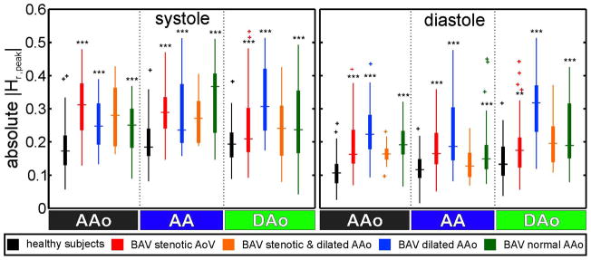
Comparison of |Hr,peak| between healthy subjects and the different patient groups shows a significant increase for the BAV patients groups during systole and diastole (** p < 0.01, *** p < 0.001).
Intra- and inter-observer analysis
Figure 8 shows the test-retest reliability using Bland-Altman plots performed for three planes in three healthy subjects and three patients which reveal moderate agreement for intra- (mean difference = −0.004, limits of agreement = ±0.08) and inter-observer analysis (mean difference = −0.002, limits of agreement = ±0.07).
Fig. 8.
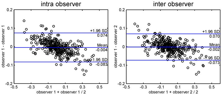
Bland-Altman plots for inter- and intra- observer reproducibility for 3 analysis planes (AAo, AA, DAo) in 3 healthy subjects and 3 patients.
Influence of venc selection
Results are shown as box plots for <Hr(t)> and <Hd(t)> for different vencs: 1.0 m/s, 1.5 m/s 2.0 m/s and 2.5 m/s in figure 9. For all vencs, the median was the same for <Hr(t)> and <Hd(t)>. For <Hr(t)>, the variance of the data and the 1.5 times the interquartile range reduces with higher venc although there are more outliers. For <Hd(t)>, the variances and the 1.5 times the interquartile range show an expected increase with higher venc with many outliers present. For venc 1.0 m/s aliased and unwrapped data is presented. For both helicity parameters the box plots appear to be similar. The aliased data shows more outliers for negative values for helicity density.
Fig. 9.
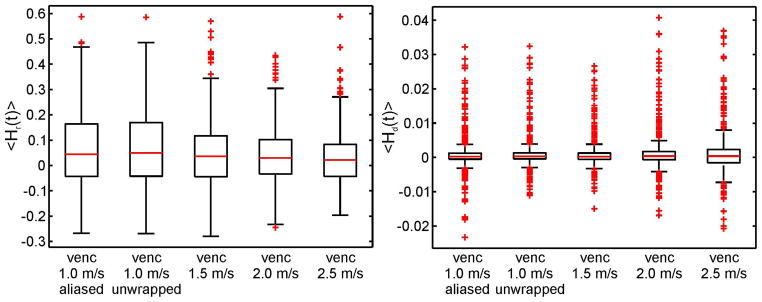
Effect of different vencs on the results of helicity quantification demonstrated by box plots of mean relative helicity in comparison to different vencs (1.0 m/s, 1.5 m/s, 2.0 m/s and 2.5 m/s). Additionally for venc 1.0 m/s, aliased and un-wrapped data is presented.
Discussion
The aim of the study was to develop and apply an adequate analysis protocol to reliably quantify helical flow. 2D planes were equally distributed along the aorta and <Hr(t)>, <Hd(t)>, <Hr>avg, <Hd>avg, and |Hr,peak| was calculated for each plane.
Healthy subjects showed consistent directions of rotation over the entire aorta with high clockwise helicity in the aortic arch. A <Hr>avg analysis over the aorta at different time steps revealed the expected increase of clockwise rotation during peak and late systole in the AA and counter-clockwise rotation in the DAo. This behavior was also observed by Kilner et al. (13) and Bogren et al. (11).
Repeated 4D flow MRI and analysis revealed a significant repeatability of <Hr(t)> within the AAo, AA and DAo. Bland-Altman analysis performed for <Hr>avg in these three sections of the aorta demonstrated a moderate repeatability of the helicity quantification with low mean difference of 0.002 and limits of agreement of ±0.06. Results of the test-retest reproducibility for one healthy subject acquired successively during one day demonstrate that time between measurements and possible involved changes of variables that could influence helicity are not crucial factors for the repeatability of the method. Both scan and rescan with varying time present similar results using Bland-Altman analysis (mean difference: 0.002 (AAo), −0.001 (AA), 0.001 (DAo)).
The remaining differences might be explained by shifted and tilted slice positioning since all analysis planes had to be manually placed along the aorta for both acquisitions. Future studies might thus benefit from a more automated and fully three-dimensional analysis which would avoid manual user interaction as a source of inaccuracy.
We further assume that the moderate results for the test-retest repeatability of the helicity data is due to the sensitivity of our helicity calculation method to small changes such as noise, the position of the analysis plane and even the segmentation of the vessel, as shown in the inter- and intra-observer analysis. Application of a median filter or smoothing of the helicity data could help to reduce this sensitivity. However, the influence of higher vencs and therefore reduced SNR is marginal. For relative helicity, the effect of higher vencs is even lower than for smaller vencs. Errors regarding the unwrapping of the data are not expected. Unwrapping is performed in the velocity data prior to vorticity and helicity calculation.
The <Hr>avg and <Hd>avg values during systole and diastole provide information of the overall distribution of helicity and whether a single rotation direction is more prominent than the other in certain parts of the aorta (e.g. clockwise rotation in the aortic arch). In the ascending and descending aorta, there appears to be insignifant or minor <Hr>avg and <Hd>avg during systole. As expected <Hr>avg and <Hd>avg are reduced during diastole.
Temporally resolved mean relative helicity <Hr(t)> demonstrates opposite rotation behavior between the AAo and the DAo, which is supported by the findings of Kilner et al. (13) and Bogren et al. (11). The formation of the positive and negative peak in <Hr(t)> may be due to the reflected pressure wave from the distal vasculature similar to time-resolved relative pressure mapping (36). These positive and negative peaks which are observable in <Hr(t)> in the AAo and DAo may cancel out for <Hr>avg. This might lead to false conclusions about helical flow within the aorta. However, it is important to note that for retrograde flow the sign of <Hr(t)> reflects inverted rotation behavior due to the inverted flow direction. In these cases it would be essential to analyse helicity dependent on the main flow direction or to use only absolute values of helicity.
Quantification of helicity in patients with bicuspid aortic valve disease revealed the expected significant increase for <Hr>avg, <Hd>avg and |Hr,peak|.
Compared to healthy subjects, results of patients with aortic valve disease showed a considerably more heterogeneous distribution of <Hr>avg and <Hd>avg during systole and diastole over the aorta and in between the patient groups. There is also a difference between <Hr>avg and <Hd>avg in comparison to the healthy subjects where both helicity parameters show similar color coding. This is due to much higher values in helicity and speed during systole and diastole. Furthermore the plot demonstrates that in patients helical flow is also present during diastole.
Analysis and interpretation of temporally resolved helicity can be misleading during retrograde flow. Rotation direction of helicity is defined for forward flow only; with retrograde flow rotation direction inverts. However, the intensity of helicity remains the same. For analysis of temporal helicity it is thus crucial to additionally investigate the flow direction within the aorta. In subjects with retrograde flow rotation direction should be adapted to the flow direction or a helical flow analysis independent on the rotation direction should be performed. The evaluation of helicity parameters has the potential to serve as a biomarker to understand the development of aortopathies such as aneurysms. The quantification of helicity parameter allows an objective (quantitative) assessment of this flow pattern which can in future studies be used to investigate the link between the severity of helical flow and the development of aortopathy (progressive aortic dilation, development of aneurysms, dissection).
Results in figures 6 suggest that BAV patients with a normal AAo have increased helical flow leading to the conclusion that the orifice and the functioning of the aortic valve plays an important role in the formation of helical flow. However, to draw a final conclusion about the results of this data an analysis in more BAV patients with the same number of patients in each subgroups and a statistical analysis are necessary.
Therefore, future evaluations should investigate the influence of aortic valve/morphology of healthy subjects and patients on helical flow based on the assumption that the aortic valve and geometry of the aorta is important in the formation of helicity. In addition, the effect of eccentric and altered inflow pattern due to aortic valve diseases should be further investigated. Furthermore, the influence of age on helical flow formation should be analyzed since the elasticity of the aorta reduces with age which might affect 3D flow characteristics (37). Previous studies (11,38) have shown age dependent changes of hemodynamics.
Frydrychowicz et al. (38) shows an increase of the number of vortices with increasing age using qualitative helicity analysis. Moreover, helicity quantification used in combination with wall shear stress (WSS) data may be a valuable strategy for the prediction of aneurysm development or even aneurysm rupture. We speculate that an increase of helicity is dependent on specific changes in the geometry of the aorta, the aortic wall or the aortic valve. An increase of helicity can also result in secondary pathologies. Stronger helical flow exerts a stronger force on the vessel wall and creates a higher friction of blood relative to the vessel wall with the consequence of increased WSS. Depending on the individual physiological properties of the aortic vessel wall, this can involve changes in the geometry of the aorta. Additionally, the analysis of helical flow formation in already existing aneurysms with different shapes, sizes and locations within the aorta could provide insights in the growth of aneurysms.
In the present literature observations of helical flow are based on qualitative visual analysis such as the existence of clockwise and counter-clockwise rotation in the three parts of the aorta (AAo, AA and DAo) and the visual grading of helicity magnitude. This, however, is strongly observer dependent. Kilner et al. (13) and Bogren et al. (11) performed a visual analysis of helical flow within the healthy aorta using vector arrows (Kilner et al. (13)) or streamlines (Bogren et al. (11)). The results presented in our study agree with the overall findings of their studies including: the predominant clockwise rotation in the AA, the mainly opposite rotation direction in the AAo and DAo, the persistent helical flow during diastole and the change of rotation direction over the cardiac cycle. However, a quantification of helical flow provides the opportunity to present helicity values for diagnostic and comparative purposes with respect to helicity intensity and rotation direction.
Mobiducci et al (22,23) provided the first quantitative analysis of helical flow based on particle traces. A helical flow index (HFI) was calculated using the points of the particle traces for each time interval during systole. The method allows for the three dimensional coverage of the aorta, but is limited by length of the particle trace trajectories over a certain time interval. Therefore, the quantification of helicity is generally restricted to a short section of the aorta. Additionally, the particle trace generation is restricted to time intervals during systole and results are shown in absolute values of relative helicity which do not include information on clockwise or counter-clockwise rotation. In contrast, the method presented in this study allows for a large coverage of the entire aorta and over the entire cardiac cycle. This was particularly important for the helicity quantification in our patient cohort revealing strong helical flow during diastole. Furthermore, the HFI revealed values between 0.3 and 0.5 for five time points during systole of the five healthy subjects. Our study revealed much lower values for relative helicity in healthy subjects e.g. |Hr,peak| during systole was between 0.1 and 0.2.
Clough et al. (39) recently published a report where helicity was quantified by the assessment of the amount of rotation. However, the described helicity analysis is based on a semi-quantitative visual observation of the rotational movement of particle traces over time. As a result, the described methodology works well for pronounced and clear visible helical flow but is not truly quantitative and may thus be limited by observer variability. Unfortunately, the work of Clough et al. also does not provide any information on observer dependent variability of their helicity analysis. Further, Clough et al. showed the degree of rotation, but no information of the temporal evolution of helical flow was provided.
In addition, the study does not provide any results in healthy subjects or any comparison between patients and healthy subjects. Previous work (11–15) and results provided in our work show that helical flow is present in healthy subjects. For a clinical study a comparison between healthy subjects and patients is thus important to distinguish between normal and abnormal rotational flow behavior. The quantification strategy proposed in our work can be time consuming by placing several 2D planes over the aorta. However, the 2D analysis planes for helicity quantification can provide additional information such as velocity, flow or other metrics of aortic hemodynamics.
Limitations of the present study include the analysis of the three-dimensional helicity parameter by two dimensional cross sections distributed over the aorta. Depending on the distance between the cross sections, small local helical flows may remain undetected. Furthermore, our analysis strategy does not allow for the detection of different helicity formations such as duplex helical flow or small helical flow at the vessel wall due to the averaging process over all pixels in the cross section. Future development should thus include a full 3D and pixel-wise analysis of helical flow characteristics. Another limitation of this study is the absence of an age-matched control group. Nevertheless, our study clearly demonstrated the possibility of quantifying aortic flow helicity and illustrated the sensitivity of this parameter to identify altered helix flow in patients with aortic valve disease.
Additionally, in some of the patient measurements a large venc was chosen to capture the high velocities in the AAo which resulted in a poor SNR. This could be improved by a better adaptation of the venc to the actual velocities.
We assume that our approach could also be applied to vessels and branch vessels with aneurysmal disease. However, this is dependent on the size of the vessels, the type of aneurysm and the flow within the aneurysm. We speculate that, based on the spatial resolution of our methods, helicity analysis in vessels below 5–8 mm remains challenging. Changes in pulse sequence parameters, intra-vascular contrast agents and the application of new spatio-temporal imaging acceleration techniques such as k-t undersampling or compressed sensing may help to improve resolution of the assessment of helicity in smaller vessel. Future studies are warranted to evaluate the potential of these methods for the accurate assessment of hemodynamics in smaller vessels.
Conclusion
This study provides a fully quantitative analysis and detailed evaluation of the spatial and temporal distribution of helical flow (main direction and intensity of helicity) within the aorta of healthy subjects and BAV patients. We illustrated that the quantification of helical flow is feasible. The study showed a good inter-individual agreement and repeatability of the method in healthy subjects and considerable increased helical flow in BAV patients.
The method has the potential to serve as a reference distribution for comparisons of helical flow between healthy subjects and patients or between different patient groups. This study does not allow a determination of the causal factor, i.e. whether an increase of helicity creates changes in the aortic morphology/valve or vice versa. Rather, the sole research of helicity quantification or together with other 3D flow characteristics could help to understand and predict the development of aortic diseases involving modifications of the vessel wall or the aortic valve.
Acknowledgments
Grant support: NIH NHLBI grant R01HL115828; NUCATS Institute NIH grant UL1RR025741, and the Northwestern Memorial Foundation Dixon Translational Research Grants Initiative; American Heart Association Scientist Development Grant 13SDG14360004.
Footnotes
Parts of this work were presented at the ISMRM 2011 in Montreal, Canada and at the ISMRM 2012 in Melbourne, Australia
References
- 1.Chai P, Mohiaddin R. How we perform cardiovascular magnetic resonance flow assessment using phase-contrast velocity mapping. J Cardiovasc Magn Reson. 2005;7(4):705–716. doi: 10.1081/jcmr-65639. [DOI] [PubMed] [Google Scholar]
- 2.Dumoulin CL. Phase contrast MR angiography techniques. Magn Reson Imaging Clin N Am. 1995;3(3):399–411. [PubMed] [Google Scholar]
- 3.Markl M, Harloff A, Bley TA, Zaitsev M, Jung B, Weigang E, Langer M, Hennig J, Frydrychowicz A. Time-resolved 3D MR velocity mapping at 3T: improved navigator-gated assessment of vascular anatomy and blood flow. J Magn Reson Imaging. 2007;25(4):824–831. doi: 10.1002/jmri.20871. [DOI] [PubMed] [Google Scholar]
- 4.Uribe S, Beerbaum P, Sorensen TS, Rasmusson A, Razavi R, Schaeffter T. Four-dimensional (4D) flow of the whole heart and great vessels using real-time respiratory self-gating. Magn Reson Med. 2009;62(4):984–992. doi: 10.1002/mrm.22090. [DOI] [PubMed] [Google Scholar]
- 5.Wigstrom L, Sjoqvist L, Wranne B. Temporally resolved 3D phase-contrast imaging. Magn Reson Med. 1996;36(5):800–803. doi: 10.1002/mrm.1910360521. [DOI] [PubMed] [Google Scholar]
- 6.Frydrychowicz A, Harloff A, Jung B, Zaitsev M, Weigang E, Bley TA, Langer M, Hennig J, Markl M. Time-resolved, 3-dimensional magnetic resonance flow analysis at 3 T: visualization of normal and pathological aortic vascular hemodynamics. Journal of computer assisted tomography. 2007;31(1):9–15. doi: 10.1097/01.rct.0000232918.45158.c9. [DOI] [PubMed] [Google Scholar]
- 7.Frydrychowicz A, Markl M, Hirtler D, Harloff A, Schlensak C, Geiger J, Stiller B, Arnold R. Aortic hemodynamics in patients with and without repair of aortic coarctation: in vivo analysis by 4D flow-sensitive magnetic resonance imaging. Investigative radiology. 2011;46(5):317–325. doi: 10.1097/RLI.0b013e3182034fc2. [DOI] [PubMed] [Google Scholar]
- 8.Hope TA, Markl M, Wigstrom L, Alley MT, Miller DC, Herfkens RJ. Comparison of flow patterns in ascending aortic aneurysms and volunteers using four-dimensional magnetic resonance velocity mapping. J Magn Reson Imaging. 2007;26(6):1471–1479. doi: 10.1002/jmri.21082. [DOI] [PubMed] [Google Scholar]
- 9.Markl M, Draney MT, Hope MD, Levin JM, Chan FP, Alley MT, Pelc NJ, Herfkens RJ. Time-resolved 3-dimensional velocity mapping in the thoracic aorta: visualization of 3-directional blood flow patterns in healthy volunteers and patients. Journal of computer assisted tomography. 2004;28(4):459–468. doi: 10.1097/00004728-200407000-00005. [DOI] [PubMed] [Google Scholar]
- 10.Markl M, Draney MT, Miller DC, Levin JM, Williamson EE, Pelc NJ, Liang DH, Herfkens RJ. Time-resolved three-dimensional magnetic resonance velocity mapping of aortic flow in healthy volunteers and patients after valve-sparing aortic root replacement. The Journal of thoracic and cardiovascular surgery. 2005;130(2):456–463. doi: 10.1016/j.jtcvs.2004.08.056. [DOI] [PubMed] [Google Scholar]
- 11.Bogren HG, Buonocore MH. 4D magnetic resonance velocity mapping of blood flow patterns in the aorta in young vs. elderly normal subjects. J Magn Reson Imaging. 1999;10(5):861–869. doi: 10.1002/(sici)1522-2586(199911)10:5<861::aid-jmri35>3.0.co;2-e. [DOI] [PubMed] [Google Scholar]
- 12.Buonocore MH, Bogren HG. Analysis of flow patterns using MRI. International journal of cardiac imaging. 1999;15(2):99–103. doi: 10.1023/a:1006205206534. [DOI] [PubMed] [Google Scholar]
- 13.Kilner PJ, Yang GZ, Mohiaddin RH, Firmin DN, Longmore DB. Helical and retrograde secondary flow patterns in the aortic arch studied by three-directional magnetic resonance velocity mapping. Circulation. 1993;88(5 Pt 1):2235–2247. doi: 10.1161/01.cir.88.5.2235. [DOI] [PubMed] [Google Scholar]
- 14.Seed WA, Wood NB. Velocity patterns in the aorta. Cardiovascular research. 1971;5(3):319–330. doi: 10.1093/cvr/5.3.319. [DOI] [PubMed] [Google Scholar]
- 15.Segadal L, Matre K. Blood velocity distribution in the human ascending aorta. Circulation. 1987;76(1):90–100. doi: 10.1161/01.cir.76.1.90. [DOI] [PubMed] [Google Scholar]
- 16.Hope MD, Hope TA, Crook SE, Ordovas KG, Urbania TH, Alley MT, Higgins CB. 4D flow CMR in assessment of valve-related ascending aortic disease. Jacc. 4(7):781–787. doi: 10.1016/j.jcmg.2011.05.004. [DOI] [PubMed] [Google Scholar]
- 17.Hope MD, Hope TA, Meadows AK, Ordovas KG, Urbania TH, Alley MT, Higgins CB. Bicuspid aortic valve: four-dimensional MR evaluation of ascending aortic systolic flow patterns. Radiology. 2010;255(1):53–61. doi: 10.1148/radiol.09091437. [DOI] [PubMed] [Google Scholar]
- 18.Barker AJ, Markl M, Burk J, Lorenz R, Bock J, Bauer S, Schulz-Menger J, von Knobelsdorff-Brenkenhoff F. Bicuspid aortic valve is associated with altered wall shear stress in the ascending aorta. Circ Cardiovasc Imaging. 2012;5(4):457–466. doi: 10.1161/CIRCIMAGING.112.973370. [DOI] [PubMed] [Google Scholar]
- 19.Malek AM, Alper SL, Izumo S. Hemodynamic shear stress and its role in atherosclerosis. Jama. 1999;282(21):2035–2042. doi: 10.1001/jama.282.21.2035. [DOI] [PubMed] [Google Scholar]
- 20.Hope MD, Hope TA, Crook SE, Ordovas KG, Urbania TH, Alley MT, Higgins CB. 4D flow CMR in assessment of valve-related ascending aortic disease. Jacc. 2011;4(7):781–787. doi: 10.1016/j.jcmg.2011.05.004. [DOI] [PubMed] [Google Scholar]
- 21.Frydrychowicz A, Weigang E, Langer M, Markl M. Flow-sensitive 3D magnetic resonance imaging reveals complex blood flow alterations in aortic Dacron graft repair. Interactive cardiovascular and thoracic surgery. 2006;5(4):340–342. doi: 10.1510/icvts.2006.129577. [DOI] [PubMed] [Google Scholar]
- 22.Morbiducci U, Ponzini R, Rizzo G, Cadioli M, Esposito A, De Cobelli F, Del Maschio A, Montevecchi FM, Redaelli A. In vivo quantification of helical blood flow in human aorta by time-resolved three-dimensional cine phase contrast magnetic resonance imaging. Ann Biomed Eng. 2009;37(3):516–531. doi: 10.1007/s10439-008-9609-6. [DOI] [PubMed] [Google Scholar]
- 23.Morbiducci U, Ponzini R, Rizzo G, Cadioli M, Esposito A, Montevecchi FM, Redaelli A. Mechanistic insight into the physiological relevance of helical blood flow in the human aorta: an in vivo study. Biomech Model Mechanobiol. 2010;10(3):339–355. doi: 10.1007/s10237-010-0238-2. [DOI] [PubMed] [Google Scholar]
- 24.Erbel R, Alfonso F, Boileau C, Dirsch O, Eber B, Haverich A, Rakowski H, Struyven J, Radegran K, Sechtem U, Taylor J, Zollikofer C, Klein WW, Mulder B, Providencia LA. Diagnosis and management of aortic dissection. European heart journal. 2001;22(18):1642–1681. doi: 10.1053/euhj.2001.2782. [DOI] [PubMed] [Google Scholar]
- 25.Bonow RO, Carabello BA, Chatterjee K, de Leon AC, Jr, Faxon DP, Freed MD, Gaasch WH, Lytle BW, Nishimura RA, O’Gara PT, O’Rourke RA, Otto CM, Shah PM, Shanewise JS. 2008 Focused update incorporated into the ACC/AHA 2006 guidelines for the management of patients with valvular heart disease: a report of the American College of Cardiology/American Heart Association Task Force on Practice Guidelines (Writing Committee to Revise the 1998 Guidelines for the Management of Patients With Valvular Heart Disease): endorsed by the Society of Cardiovascular Anesthesiologists, Society for Cardiovascular Angiography and Interventions, and Society of Thoracic Surgeons. Circulation. 2008;118(15):e523–661. doi: 10.1161/CIRCULATIONAHA.108.190748. [DOI] [PubMed] [Google Scholar]
- 26.von Knobelsdorff-Brenkenhoff F, Rudolph A, Wassmuth R, Abdel-Aty H, Schulz-Menger J. Aortic dilatation in patients with prosthetic aortic valve: comparison of MRI and echocardiography. The Journal of heart valve disease. 19(3):349–356. [PubMed] [Google Scholar]
- 27.Lotz J, Doker R, Noeske R, Schuttert M, Felix R, Galanski M, Gutberlet M, Meyer GP. In vitro validation of phase-contrast flow measurements at 3 T in comparison to 1. 5 T: precision, accuracy, and signal-to-noise ratios. J Magn Reson Imaging. 2005;21(5):604–610. doi: 10.1002/jmri.20275. [DOI] [PubMed] [Google Scholar]
- 28.Bernstein MA, Zhou XJ, Polzin JA, King KF, Ganin A, Pelc NJ, Glover GH. Concomitant gradient terms in phase contrast MR: analysis and correction. Magn Reson Med. 1998;39(2):300–308. doi: 10.1002/mrm.1910390218. [DOI] [PubMed] [Google Scholar]
- 29.Bock J, Kreher BW, Hennig J, Markl M. Optimized pre-processing of time-resolved 2D and 3D Phase Contrast MRI data. Proceedings of 15th Scientific Meeting International Society for Magnetic Resonance in Medicine; Berlin, Germany. 2007. p. 3138. [Google Scholar]
- 30.Walker PG, Cranney GB, Scheidegger MB, Waseleski G, Pohost GM, Yoganathan AP. Semiautomated method for noise reduction and background phase error correction in MR phase velocity data. J Magn Reson Imaging. 1993;3(3):521–530. doi: 10.1002/jmri.1880030315. [DOI] [PubMed] [Google Scholar]
- 31.Bock J, Frydrychowicz A, Stalder AF, Bley TA, Burkhardt H, Hennig J, Markl M. 4D phase contrast MRI at 3 T: effect of standard and blood-pool contrast agents on SNR, PC-MRA, and blood flow visualization. Magn Reson Med. 2010;63(2):330–338. doi: 10.1002/mrm.22199. [DOI] [PubMed] [Google Scholar]
- 32.Moffatt HK. The degree of knottedness of tangled vortex lines. J Fluid Mech. 1969;35(1):117–129. [Google Scholar]
- 33.Moffatt HK, Tsinober A. Helicity in laminar and turbulent flow. Annu Rev Fluid Mech. 1992;24:281–312. [Google Scholar]
- 34.Stalder AF, Russe MF, Frydrychowicz A, Bock J, Hennig J, Markl M. Quantitative 2D and 3D Phase Contrast MRI: Optimized Analysis of Blood Flow and Vessel Wall Parameters. Magn Reson Med. 2008;60(5):1218–1231. doi: 10.1002/mrm.21778. [DOI] [PubMed] [Google Scholar]
- 35.Bland JM, Altman DG. Statistical methods for assessing agreement between two methods of clinical measurement. Lancet. 1986;1(8476):307–310. [PubMed] [Google Scholar]
- 36.Tyszka JM, Laidlaw DH, Asa JW, Silverman JM. Three-dimensional, time-resolved (4D) relative pressure mapping using magnetic resonance imaging. J Magn Reson Imaging. 2000;12(2):321–329. doi: 10.1002/1522-2586(200008)12:2<321::aid-jmri15>3.0.co;2-2. [DOI] [PubMed] [Google Scholar]
- 37.Bader H. Dependence of wall stress in the human thoracic aorta on age and pressure. Circulation research. 1967;20(3):354–361. doi: 10.1161/01.res.20.3.354. [DOI] [PubMed] [Google Scholar]
- 38.Frydrychowicz A, Berger A, Munoz Del Rio A, Russe MF, Bock J, Harloff A, Markl M. Interdependencies of aortic arch secondary flow patterns, geometry, and age analysed by 4-dimensional phase contrast magnetic resonance imaging at 3 Tesla. European radiology. 2012;22(5):1122–1130. doi: 10.1007/s00330-011-2353-6. [DOI] [PubMed] [Google Scholar]
- 39.Clough RE, Waltham M, Giese D, Taylor PR, Schaeffter T. A new imaging method for assessment of aortic dissection using four-dimensional phase contrast magnetic resonance imaging. Journal of vascular surgery. 55(4):914–923. doi: 10.1016/j.jvs.2011.11.005. [DOI] [PubMed] [Google Scholar]