Variational Implicit Solvation with Solute Molecular Mechanics: From Diffuse-Interface to Sharp-Interface Models

Abstract

Central in a variational implicit-solvent description of biomolecular solvation is an effective free-energy functional of the solute atomic positions and the solute-solvent interface (i.e., the dielectric boundary). The free-energy functional couples together the solute molecular mechanical interaction energy, the solute-solvent interfacial energy, the solute-solvent van der Waals interaction energy, and the electrostatic energy. In recent years, the sharp-interface version of the variational implicit-solvent model has been developed and used for numerical computations of molecular solvation. In this work, we propose a diffuse-interface version of the variational implicit-solvent model with solute molecular mechanics. We also analyze both the sharp-interface and diffuse-interface models. We prove the existence of free-energy minimizers and obtain their bounds. We also prove the convergence of the diffuse-interface model to the sharp-interface model in the sense of Γ-convergence. We further discuss properties of sharp-interface free-energy minimizers, the boundary conditions and the coupling of the Poisson–Boltzmann equation in the diffuse-interface model, and the convergence of forces from diffuse-interface to sharp-interface descriptions. Our analysis relies on the previous works on the problem of minimizing surface areas and on our observations on the coupling between solute molecular mechanical interactions with the continuum solvent. Our studies justify rigorously the self consistency of the proposed diffuse-interface variational models of implicit solvation.

1 Introduction

The interaction between biomolecules (such as proteins, nucleic acids, and lipid membranes) and their surrounding aqueous solvent (such as water or salted water) contributes significantly to the structure, dynamics, and functions of an underlying biomolecular system. Such interactions can be described efficiently by implicit-solvent (or continuum-solvent) models [19, 37]. In such a model, the solvent molecules and ions are treated implicitly and their effects are coarse-grained; cf. Figure 1. The description of the solvent is thus reduced to that of the solute-solvent interface (i.e., the dielectric boundary) and the related macroscopic quantities, such as the surface tension, dielectric coefficients, and bulk solvent density. Implicit-solvent models are complementary to the more accurate but also more expensive explicit-solvent models such as molecular dynamics simulations, which often provide sampled statistical information rather than direct thermodynamic descriptions.

Figure 1.

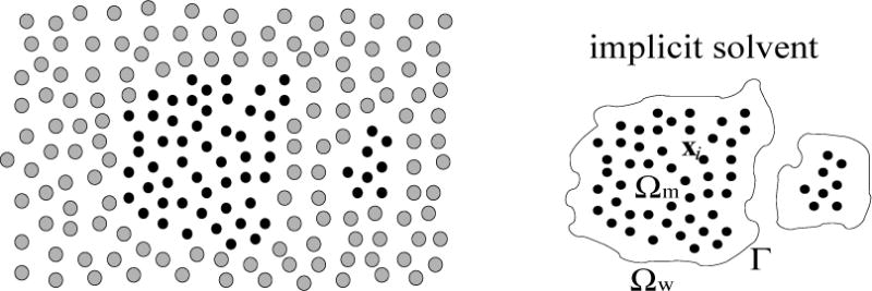
Schematic descriptions of a solvation system. Left: In a fully atomistic model, both the solute atoms (small and dark dots) and solvent molecules (large and grey dots) are degrees of freedom of the system. Right: In an implicit-solvent model, the solvent molecules are coarse-grained and the solvent is treated as a continuum. The solvent region Ω_w and the solute region Ω_m are separated by the solute-solvent interface (i.e., the dielectric boundary) Γ. The solute atoms are located at x₁, …, x_N inside Ω_m.

With an implicit solvent, the conformation of a biomolecular system in equilibrium is described by all the atomic positions of solute molecules together with the solute-solvent interface. In the recently developed variational implicit-solvent model, such equilibrium solute atomic positions and solute-solvent interfaces are defined to minimize an effective free-energy functional; cf. [15, 16] and [11, 43] for more details. In a simple setting, the free-energy functional has the form

$$F[X,\mathrm{\Gamma }]=E[X]+\gamma \text{Area}(\mathrm{\Gamma })+{{\displaystyle \int }}_{\mathrm{\Omega }\text{w}}U(X,x)dx.$$ (1.1)

Here the first term E[X]is the potential energy of molecular mechanical interactions of solute atoms located at x₁, …, x_N inside the solute region Ω_m (cf. Figure 1) and X = (x₁, …, x_N). The molecular mechanical interactions include the chemical bonding, bending, and torsion; the short-distance repulsion and the long-distance attraction; and the Coulombic charge-charge interaction.

The second term is an effective surface energy of the solute-solvent interface Γ that separates the solute region Ω_m from the solvent region Ω_w, where γ is an effective surface energy density assumed to be a constant. (The subscripts m and w stand for molecule and water, respectively.)

The last term models the solute-solvent interactions by an interaction potential U(X, x) that is defined on all (X, x) with $X=(x_1,\dots ,x_N)\in {\mathrm{\Omega }}_{\text{m}}^N({\mathrm{\Omega }}_{\text{m}}^N={\mathrm{\Omega }}_{\text{m}}\times \cdots \times {\mathrm{\Omega }}_{\text{m}}\text{ with }N\text{ copies})$ ) and x ∈ Ω_w. There are mainly two types of solute-solvent interactions. One is the non-electrostatic dispersive interaction that includes the repulsion due to the excluded-volume effect and the van der Waals attraction. Such interactions can be modeled by ρ_wU_vdW, where ρ_w is the bulk solvent density and U_vdW is the potential defined by

$$U_{\text{vdW}}(X,x)=\sum _{i=1}^N{U}_i(|x-x_i|).$$ (1.2)

Here, each U_i (|x − x_i|) is the interaction potential between the solute particle at x_i and a solvent molecule or an ion located at x ∈ Ω_w. Practically, one can take the pairwise interaction U_i to be a Lennard-Jones potential

$$U_i(r)=4{\epsilon }_i[{\left(\frac{{\sigma }_i}{r}\right)}^{12}-{\left(\frac{{\sigma }_i}{r}\right)}^6]$$

with ε_i and σ_i being effective parameters. The other is the electrostatic interaction for which the solute-solvent interface Γ is used as the dielectric boundary. In an implicit-solvent approach, the electrostatic interaction energy is often obtained by solving the Poisson–Boltzmann equation [12, 21, 24, 31, 40]. However, by using the Coulomb-field or Yukawa-field approximation, we can obtain, without solving the Poisson–Boltzmann equation, good approximations of the electrostatic interaction energy [7, 43]. In the Coulomb-field approximation, the electrostatic energy density is given by [43]

$$U_{\text{ele}}(X,x)=\frac{1}{32{\pi }^2{\epsilon }_v}(\frac{1}{{\epsilon }_w}-\frac{1}{{\epsilon }_m})|{\displaystyle \sum }_{i=1}^N\frac{Q_i(x-x_i)}{|x-x_i{|}^3}{|}^2,$$

where ε_v is the vacuum permittivity (often denoted by ε₀ in literature), ε_m and ε_w are the relative permittivities of the solute and solvent, respectively, and Q_i is the charge carried by the solute atom located at x_i. (Typical values of ε_m and ε_w are around 1 and 80, respectively) The total solute-solvent interaction potential is then given by

$$\begin{array}{cc}U(X,x)={\rho }_{\text{w}}{U}_{\text{vdW}}(X,x)+U_{\text{ele}}(X,x),& X\end{array}\in {\mathrm{\Omega }}_{\text{m}}^N,x\in {\mathrm{\Omega }}_{\text{w}}.$$ (1.3)

For a fixed set of solute atoms X = (x₁, …, x_N), a solute-solvent interface Γ with a low free energy tends to minimize its surface area. On the other hand, the solute-solvent interaction modeled by the third term in (1.1) prevents the interface from being too close to the solute atoms located at x_i (1 ≤ i ≤ N).

In [8], Cheng et al. developed a robust level-set method to minimize numerically the free-energy functional (1.1) for a fixed set of solute atoms X. The idea is to move an initially guessed solute-solvent interface that may have a large free energy in the direction of steepest descent of free energy until a (local) minimizer is reached. The “velocity” of the moving interface is therefore given by the effective interface or boundary force that is defined to be the negative variational derivative of the free-energy functional with respect to the location change of the interface. This method has been improved, generalized, and applied to many more systems ranging from small molecules to proteins [9–11, 38, 43]. Extensive numerical results with comparison with molecular dynamics simulations have demonstrated the success of the level-set variational solvation in capturing the hydrophobic interaction, multiple equilibrium states of hydration, and fluctuations between such states.

In this work, we first propose a diffuse-interface variational implicit-solvent model, as an alternative to the original variational implicit-solvent model that uses a sharp-interface formulation, for molecular solvation. We then prove that the diffuse-interface model converges to the corresponding sharp-interface model in the sense of Γ-convergence.

Diffuse-interface approaches have been widely used in studying interface problems arising in many scientific areas, such as materials physics, complex fluids, and biomembranes, cf. e.g., [1, 4, 5, 14, 17, 22, 25, 30, 39] and the references therein. In a diffuse-interface model, an interface separating two regions is represented by a continuous function that takes values close to one constant in one of the regions and another constant in the other region, but smoothly changes its values from one of the constants to another in a thin transition region. Both the sharp-interface and the diffuse-interface approaches have their own advantages and disadvantages. Existing studies have shown that interfacial fluctuations can be described in a diffuse-interface approach [3, 26]. Such fluctuations are particularly crucial in the transition of one equilibrium conformation to another in a biomolecular system.

Our diffuse-interface model is governed by the effective free-energy functional

$$F_{\epsilon }[X,\varphi ]=E[X]+\gamma {{\displaystyle \int }}_{\mathrm{\Omega }}\left[\frac{\epsilon }{2}|\nabla \varphi (x){|}^2+\frac{1}{\epsilon }W(\varphi (x))\right]dx+{{\displaystyle \int }}_{\mathrm{\Omega }}{[\varphi (x)-1]}^{2}U(X,x)dx.$$ (1.4)

Here ε > 0 is a small parameter. As in the sharp-interface variational solvation model, X = (x₁, …, x_N) and x_i is the position of the ith solute atom (1 ≤ i ≤ N). All the solute atoms are located inside the entire solvation region Ω. The function ϕ : Ω → ℝ, often called an order parameter, describes the location of solute-solvent interface. The first term E[X] is the same as in the sharp-interface model; cf. (1.1). The second term is an approximation of the surface energy of the solute-solvent interface, where the parameter γ is the constant surface energy density as before and the function W = W(s) is a double-well potential with the two wells at s = 0 and s = 1 of equal depth. The last term is the solute-solvent interaction energy with the potential U(X, x) being the same as in the sharp-interface model; cf. (1.3).

To obtain numerically equilibrium conformations of a charged molecular system, we fix the small parameter ε > 0 and solve numerically the equations of the gradient-flow of the free-energy functional (1.4),

$$\{\begin{array}{c}\dot{X}=-{\nabla }_X{F}_{\epsilon }[X,\varphi ],\\ {\partial }_t\varphi =-{\delta }_{\varphi }{F}_{\epsilon }[X,\varphi ],\end{array}$$

for X = X(t) and ϕ = ϕ(x, t). Here and below, a dot on top denotes the derivative with respect to t, ∇_X denotes the gradient with respect to X = (x₁, …, x_N), and δ_ϕ denotes the variational derivative with respect to ϕ. Explicitly, the gradient-flow equations are

$$\{\begin{array}{l}{\partial }_t\varphi =\gamma \left[\epsilon \Delta \varphi -\frac{1}{\epsilon }W\text{'}(\varphi )\right]-2(\varphi -1)U(X,\cdot )\text{ in }\mathrm{\Omega },\\ \dot{X}=-{\nabla }_{X}E[X]-{\displaystyle {{\displaystyle \int }}_{\mathrm{\Omega }}}{[\varphi (x)-1]}^2{\nabla }_{X}U(X,x)d_x.\end{array}$$ (1.5)

The second equation is equivalent to the N vector-equations

$$\begin{array}{cc}{\dot{x}}_i=-{\nabla }_{x_i}E[X]-{{{\displaystyle \int }}_{\mathrm{\Omega }}[\varphi (x)-1]}^2{\nabla }_{x_i}U(X,x)dx,& i=1,\dots ,N.\end{array}$$

In Figure 2, we show our diffuse-interface computational results of a two-plate molecular system that has been used as a prototype system in many molecular dynamics and continuum simulations [8, 9, 28, 29, 33, 43]. Each plate consists of 6 × 6 neutral atoms that are fixed in each of the two computations. We observe that the diffuse-interface model captures the two local minimizers of the system. We shall report more diffuse-interface computational results in our subsequent work.

Figure 2.

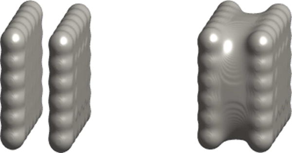
Numerical computations of a two-plate system based on the diffuse-interface version of the variational implicit-solvent model. Left: a tight-wrap equilibrium conformation. Right: a dewetting equilibrium conformation.

The main body of this work is an analysis of the variational implicit-solvent models, both the sharp-interface and the diffuse-interface versions, for molecular solvation. Specifically, we prove the following:

1. The sharp-interface free-energy functional F = F[X, Γ], defined in (1.1), is minimized by a set of solute atoms X and the boundary of a measurable subset A ⊆ Ω that has a finite perimeter in Ω. Moreover, the minimum free energy can be approximated by boundaries of sets that contain small balls centered at x_i (1 ≤ i ≤ N); cf. Theorem 2.1 and Theorem 2.2;

2. The existence of free-energy minimizers of the diffuse-interface free-energy functionals F_ε, defined in (1.4), and the bounds on such minimizers and on the minimum free energies; cf. Theorem 3.1;

3. The convergence of the minimum free energies and the free-energy minimizers of the diffuse-interface free-energy functional (1.4) to those of the corresponding sharp-interface free-energy functional (1.1); cf. Theorem 4.1, Theorem 4.2, and Theorem 4.3.

In addition, we discuss several issues. These include the regularity and other properties of sharp-interface free-energy minimizers, the boundary conditions in the diffuse-interface model, the convergence of the diffuse-interface forces to the sharp-interface forces, and the coupling of the Poisson–Boltzmann description of the electrostatic interaction in the diffuse-interface modeling. We discuss both the forces acting on the solute atoms and the dielectric boundary forces.

Our analysis relies on some of the properties of the underlying models, in particular, the interplay between the solute particles X and the field ϕ, and on the existing studies on the diffuse-interface approximations of the motion by mean curvature with the constant-volume constraint [27, 34, 35, 41].

We notice that a diffuse-interface model for solvation is proposed in [6], where the surface energy is modeled by the integral of γ|∇S| with γ being the surface energy density and S a field similar to our ϕ. However, there are no terms in the total free-energy functional G_total (cf. Eq. (7) in [6]) that can keep the field S to be close to two distinct values so that the system region can be partitioned into the solute and solvent regions by the field S. Unless an equilibrium boundary or field S is a priori known, the minimization of the total free-energy functional will smooth out the field S to reduce the surface energy.

In Section 2, we describe the main assumptions on the interaction potentials E[X] and U(X, x). We also prove the existence of minimizers for the sharp-interface free-energy functional (1.1). In Section 3, we prove the existence of minimizers for the diffuse-interface free-energy functional (1.4). We also prove some properties of such minimizers. In Section 4, we prove the convergence of the minimum free energies and free-energy minimizers in passing the diffuse-interface to the sharp-interface description. Some lemmas are used in the proof. These lemmas are proved in the Appendix. Finally, in Section 5, we discuss several issues on the properties of sharp-interface free-energy minimizers, the boundary conditions, the convergence of forces, and the coupling of the Poisson–Boltzmann equation in the diffuse-interface modeling.

2 Sharp-Interface Free-Energy Minimizers

Let Ω be a nonempty, open, connected, and bounded subset of ℝ³ with a Lipschitz-continuous boundary ∂Ω. We use an overline to denote the closure of a set. So, $\overline{\mathrm{\Omega }}$ is the closure of Ω in ℝ³. Let N > 1 be an integer and denote

$$O_N=\{X=(x_1,\cdots ,x_N)\in {({ℝ}^3)}^N:x_i\ne x_j\text{ if }i\ne j\text{ for 1}\le i,j\le N\}.$$

Clearly O_N is an open subset of (ℝ³)^N. Let $E:{\overline{\mathrm{\Omega }}}^N\to ℝ\cup \{+\infty \}$ satisfy the following

• Assumptions on E:

  • (E1) $E[X]=+\infty \text{ if }X\in {\overline{\mathrm{\Omega }}}^N\backslash ({\mathrm{\Omega }}^N\cap O_N)$ and E[X] is finite if X ∈ Ω^N ⋂ O_N. Moreover, the restriction of E onto Ω^N ⋂ O_N is a continuous function;

  • (E2) $E_{min}:={\text{inf}}_{X\in {\overline{\mathrm{\Omega }}}^N}E(X)$ is finite;

  • (E3) E[X] → + ∞ as min_1≤i<j≤N|x_i − x_j| → 0;

  • (E4) E[X] → + ∞ as min_1≤i≤N dist (x_i, ∂Ω) → 0.

The function E = E[X] with X = (x₁, …, x_N) models the potential of the molecular mechanical interactions among the solute atoms located at x₁, …,x_N. The assumption (E1) states that E[X] = + ∞ if two different atoms occupy the same position, i.e., x_i = x_j for some i and j with i ≠ j; or an atom is on the boundary, i.e., x_i ∈ ∂Ω for some i. Part of the assumption (E1) and the assumption (E3) describe the repulsion of solute atoms. Part of the assumption (E1) and the assumption (E4) can be viewed as a consequence of the assumption that E[X] → + ∞ as ${min}_{1\le i\le N}|x_i-\overline{X}|\to 0$, where $\overline{X}=(1/N){\sum }_{i=1}^N{x}_i$ is the geometrical center of the solute atoms. This models the connectivity of these atoms as a network. In practice, the open set Ω is an underlying computational region; and the solute atoms will be always kept inside Ω.

Let $U:{\overline{\mathrm{\Omega }}}^N\times \overline{\mathrm{\Omega }}\to ℝ{{\displaystyle \cup }}^{}\{+\infty \}$ satisfy the following

• Assumptions onU:

  • (U1) $U(X,x)=+\infty \text{if}(X,x)=(x_1,\dots ,x_N,x)\in {\overline{\mathrm{\Omega }}}^{N+1}\backslash (({\mathrm{\Omega }}^N\times \overline{\mathrm{\Omega }})\cap O_{N+1})$ and U(X, x) is finite if $(X,x)\in ({\mathrm{\Omega }}^N\times \overline{\mathrm{\Omega }})\cap O_{N+1}$. Moreover, the restriction of U onto $({\mathrm{\Omega }}^N\times \overline{\mathrm{\Omega }})\cap O_{N+1}$ is a continuous function;

  • (U2) $U_{min}:={inf}_{{\overline{\mathrm{\Omega }}}^N\times \overline{\mathrm{\Omega }}}U(X,x)$ is finite;

  • (U3) U(X, x) → +∞ as min_0≤i<j≤N|x_i − x_j|→0, where x₀ = x.

The function U = U(X, x) describes the solute-solvent interactions. Part of the assumption (U1) and the assumption (U3) model the repulsion in such interactions.

We recall that a function f ∈ L¹ (Ω) is said to have bounded variations in Ω, if

$${{\displaystyle \int }}_{\mathrm{\Omega }}|\nabla f|dx:=sup\{{{\displaystyle \int }}_{\mathrm{\Omega }}f\text{ div }\mathrm{g }dx:g\in C_c^1(\mathrm{\Omega },{ℝ}^3),|g|\le 1\text{ in }\mathrm{\Omega }\}<\infty ,$$ (2.1)

where $C_c^1(\mathrm{\Omega },{ℝ}^3)$ denotes the space of all C¹-mappings from Ω to ℝ³ that are compactly supported inside Ω; cf. [18, 23, 44]. If f ∈ W^1,1(Ω) then the value defined by (2.1) is the same as ${\Vert \nabla f\Vert }_{L^1(\mathrm{\Omega })}$. The space BV(Ω) of all L¹(Ω)-functions that have bounded variations in Ω is a Banach space with the norm

$$\begin{array}{cc}{\Vert f\Vert }_{\text{BV}(\mathrm{\Omega })}:={\Vert f\Vert }_{L^1(\mathrm{\Omega })}+{{\displaystyle \int }}_{\mathrm{\Omega }}|\nabla f|dx& \forall f\in BV(\mathrm{\Omega }).\end{array}$$

For any A ⊆ ℝ³, we denote by χ_A the characteristic function of A : χ_A(x) = 1 if x ∈ A and χ_a(x) = 0 if x ∉ A. If A is Lebesgue measurable, then the perimeter of A in Ω is defined by [18, 23, 44]

$$P_{\mathrm{\Omega }}(A):={{\displaystyle \int }}_{\mathrm{\Omega }}|{\nabla }_{\chi A}|dx.$$

We denote

$$M_0=\left\{(X,A):X\in {\overline{\mathrm{\Omega }}}^N,A\subseteq \mathrm{\Omega },A\text{ is Lebesgue measurable}\right\}.$$

Let γ > 0 be given. For any (X, A) ∈ M₀, we define

$$F_0[X,A]=E[X]+\gamma P_{\mathrm{\Omega }}(A)+{{\displaystyle \int }}_{\mathrm{\Omega }\backslash A}U(X,x)dx.$$ (2.2)

Since E and U are bounded below, F₀(X, A)> −∞. If A ⊂ Ω is open and smooth, with a finite perimeter in Ω, then F₀(X, A) = F(X, Γ), where Γ = ∂A and F is defined in (1.1) with Ω_w = Ω\A. Therefore, F₀ : M₀ → ℝ∪ {+∞} describes the free energy of a solvation system with A being the solute region.

We denote by B(y, r) the open ball in ℝ³ centered at y ∈ ℝ³ with radius r > 0. For convenience in the analysis of the solute effect, we introduce the following

Definition 2.1

Let X = (x₁, …, x_N) ∈ Ω^N ∩ O_N and σ > 0. We call $B(X,\sigma ):={\cup }_{i=1}^{N}B(x_i,\sigma )$ a σ-core of X in Ω associated with the potential U (X, ⋅), or simply an X-core, if the following are satisfied: (1) B(X, σ) ⊆ Ω; (2) $\overline{B(x_i,\sigma )}\cap \overline{B(x_j,\sigma )}=\varnothing$ if i ≠ j; and (3) U(X, x) ≥ 0 for all x ∈ B(X, σ).

It follows from the assumption (U3) that B(X, σ) is an X-core if X ∈ Ω^N ∩ O_N and σ > 0 is sufficiently small.

Our first theorem asserts the existence of a global minimizer of the sharp-interface free-energy functional F₀:M₀ → ℝ ∪ {+∞}. This is a standard result and can be proved by the direct methods in the calculus of variations. To show how the solute atoms located at x, …, x_N can be analyzed, here we give a complete proof of the theorem.

Theorem 2.1

There exists (X, A) ∈ M₀ such that

$$F_0[X,A]=\underset{(Y,B)\in M_0}{inf}{F}_0[Y,B].$$

Moreover, this minimum value is finite.

Proof

Let $\alpha ={\inf }_{(Y,B)\in M_0}{F}_0[Y,B]$. Since E and U are bounded below, α > −∞. Fix X₀ G Ω^N∩ O_N. Let A₀ = B(X₀, σ) be an X₀-core. Then (X₀, A₀) ∈ M₀. Note that U(X₀, ⋅) is bounded on $\overline{\mathrm{\Omega }}\backslash A_0$. Hence F₀[X₀, A₀] < ∞; and α is finite. There now exist (X_k, A_k) ∈ M₀ (k = 1, 2, …) such that lim_k→∞F₀[X_k, A_k] = α and that F₀[X_k, A_k] is finite for each k ≥ 1. The lower boundedness of E and U implies that ${\{P_{\mathrm{\Omega }}(A_k)\}}_{k=1}^{\infty }$ is bounded. This further implies that the sequence

$${{\displaystyle \int }}_{\mathrm{\Omega }\backslash A_k}U(X_k,x)dx(k=1,2,\dots )$$

is bounded, and finally that ${\{E[X_k]\}}_{k=1}^{\infty }$ is bounded.

Since ${\{X_k\}}_{k=1}^{\infty }$ is bounded, it has a subsequence, not relabeled, such that X_k → X as k → ∞ for some $X\in {\overline{\mathrm{\Omega }}}^N$. It follows from the boundedness of ${\{E[X_k]\}}_{k=1}^{\infty }$ and our assumptions on E that X ∈ Ω^N ∩ O_N. Moreover, the continuity of E at X implies that

$$\underset{k\to \infty }{lim}E[X_k]=E[X].$$ (2.3)

By the boundedness of ${\{P_{\mathrm{\Omega }}(A_k)\}}_{k=1}^{\infty }$ and the compact embedding BV(Ω)↪L¹ (Ω), there exists a subsequence of {χA_k}, not relabeled, such that χA_k → χa in L¹ (Ω) for some Lebesgue measurable set A ⊆ Ω. Moreover,

$$P_{\mathrm{\Omega }}(A)\le \underset{k\to \infty }{liminf}{P}_{\mathrm{\Omega }}(A_k).$$ (2.4)

Clearly (X, A) ∈ M₀. Passing to a further subsequence of ${\{{\chi \text{A}}_k\}}_{k=1}^{\infty }$ if necessary, we may assume that χA_k → χA a.e. in Ω. Applying Fatou’s Lemma and using the fact that χA_k → χa in L¹ (Ω), we obtain

$$\begin{array}{c}\underset{k\to \infty }{liminf}{{\displaystyle \int }}_{\mathrm{\Omega }\backslash A_k}U(X_k,x)dx=\underset{k\to \infty }{liminf}\left\{{{\displaystyle \int }}_{\mathrm{\Omega }}{\chi }_{\mathrm{\Omega }\backslash A_k}(x)[U(X_k,x)-U_{min}]dx+{{\displaystyle \int }}_{\mathrm{\Omega }}{\chi }_{\mathrm{\Omega }\backslash A_k}(x)U_{min}dx\right\}\\ =\underset{k\to \infty }{liminf}{{\displaystyle \int }}_{\mathrm{\Omega }}{\chi }_{\mathrm{\Omega }\backslash A_k}(x)[U(X_{k,x})-U_{min}]dx+\underset{k\to \infty }{lim}{{\displaystyle \int }}_{\mathrm{\Omega }}{\chi }_{\mathrm{\Omega }\backslash A_k}(x)U_{min}dx\\ \ge {{\displaystyle \int }}_{\mathrm{\Omega }}{\chi }_{\mathrm{\Omega }\backslash A}(x)[U(X,x)-Umin]dx+{{\displaystyle \int }}_{\mathrm{\Omega }}{\chi }_{\mathrm{\Omega }\backslash A_k}(x)U_{min}dx\\ ={{\displaystyle \int }}_{\mathrm{\Omega }\backslash A}U(X,x)dx.\end{array}$$ (2.5)

Now (2.3), (2.4), and (2.5) imply

$$F_0[X,A]\le \underset{k\to \infty }{liminf}{F}_0[X_k,A_k].$$

Hence F₀[X, A] = α. Q.E.D.

We now prove that the minimum value of the free-energy functional F₀ : M₀ → ℝ∪ {+∞} can be approximated by free energies of certain “regular” subsets. To this end, we denote by A₀ the class of subsets E∩Ω such that

1. E is an open subset of ℝ³ with a nonempty compact, C^∞ boundary ∂E;

2. ∂E ∩ Ω is C²;

3. H₂(∂E ∩ ∂Ω) = 0.

Here and below H₂(S) denotes the 2-dimensional Hausdorff measure of a set S ⊆ ℝ³. We denote

$$R_0=\{(X,A)\in M_0:X\in {\mathrm{\Omega }}^N\cap O_N,A\in A_0,\text{and A contains an X-core}\}.$$ (2.6)

Theorem 2.2

We have

$$\underset{(X,A)\in M_0}{inf}{F}_0[X,A]=\underset{(X,A)\in R_0}{inf}{F}_0[X,A].$$ (2.7)

To prove this theorem, we need two lemmas. We denote by σ_k ↓ 0 to mean that σ₁ >…> σ_k>… and lim_k→∞σ_k = 0.

Lemma 2.1

Let (X, A) ∈ M₀. Let σ_k > 0 (k = 1, 2, …) be such that σ_k ↓ 0 and that B(X, σ_k) (k = 1, 2, …) are all X-cores. We have

$$\underset{k\to \infty }{limsup}{F}_0[X,A\cup B(X,{\sigma }_k)]\le F_0[X,A].$$ (2.8)

Proof

If F₀[X, A] = ∞ then (2.8) is true. Assume F₀[X, A] < ∞. Since both E and U are bounded below, this implies that P_Ω(A) < ∞. Moreover,

$$\begin{array}{c}\underset{k\to \infty }{limsup}{P}_{\mathrm{\Omega }}(A\cup B(X,{\sigma }_k))\le \underset{k\to \infty }{limsup}[P_{\mathrm{\Omega }}(A)+P_{\mathrm{\Omega }}(B(X,{\sigma }_k))]\\ =P_{\mathrm{\Omega }}(A)+\underset{k\to \infty }{lim}{P}_{\mathrm{\Omega }}(B(X,{\sigma }_k))=P_{\mathrm{\Omega }}(A).\end{array}$$ (2.9)

It is easy to verify that for each k ≥ 1 that

$$\mathrm{\Omega }\backslash A=[\mathrm{\Omega }\backslash (A\cup B(X,{\sigma }_k))]\cup [B(X,{\sigma }_k)\backslash A]\text{ and }[\mathrm{\Omega }\backslash (A\cup B(X,{\sigma }_k))]\cap [B(X,{\sigma }_k)\backslash A]=\varnothing .$$

Since U(X, x) ≥ 0 for all x ∈ B(X, σ_k) for each k ≥ 1, we then have

$$\begin{array}{c}{{\displaystyle \int }}_{\mathrm{\Omega }\backslash (A\cup B(X,{\sigma }_k))}U(X,x)dx\le {{\displaystyle \int }}_{\mathrm{\Omega }\backslash (A\cup B(X,{\sigma }_k))}U(X,x)dx+{{\displaystyle \int }}_{B(X,{\sigma }_k\backslash A)}U(X,x)dx\\ ={{\displaystyle \int }}_{\mathrm{\Omega }\backslash A}U(X,x)dx,k=1,2\dots \end{array}$$

This, (2.9), and (2.2) (the definition of F₀) imply (2.8) Q.E.D.

Lemma 2.2

Let (X, A) ∈ M₀ be such that X ∈ Ω^N ∩ O_N, P_Ω(A) < ∞, and A contains an X-core. Then for each integer k ≥ 1 there exists A_k ⊆ A₀ such that A_k contains an X-core, and

$$\underset{k\to \infty }{lim}{F}_0[X,A_k]=F_0[X,A].$$ (2.10)

This lemma is very similar to Lemma 1 in [34] and Lemma 1 in [41]. The volume constraint there, which gives rise to rather technical difficulties, is replaced here by the integral term in the free-energy functional F₀.

Proof of Lemma 2.2

Assume A contains an X-core B(X, σ). Since P_Ω(A)< ∞, there exists u ∈ BV (ℝ³) ∩ L^∞(ℝ³) such that u = χ_A in Ω and

$${{\displaystyle \int }}_{\partial \mathrm{\Omega }}|\nabla u|dx=0;$$ (2.11)

cf. (3) in [34]. Notice that u = 1on B(X, σ). By using mollifiers, we can construct u_k ∈ C^∞(ℝ³) (k = 1, 2, …) such that u_k = 1 in B(X, σ/2) (k = 1, 2, …), u_k → u in L¹(Ω), and using (2.11)

$$\underset{k\to \infty }{lim}{{\displaystyle \int }}_{\mathrm{\Omega }}|\nabla u_k|dx={{\displaystyle \int }}_{\mathrm{\Omega }}|\nabla u|dx=P_{\mathrm{\Omega }}(A);$$

cf. Sections 2.8 and 2.16 in [23]. For a given t ∈ ℝ, we define E_k = {x ∈ ℝ³: u_k(x) > t} (k = 1, 2, …). Clearly, each E_k is an open subset of ℝ³. Following the proof of Lemma 1 in [34] and Lemma 1 in [41], there exists t ∈ (0, 1) and a subsequence of ${\{E_k\}}_{k=1}^{\infty }$, not relabeled, that satisfy the following properties: (1) For each k ≥ 1, E_k ⊇ B(X, σ/2); (2) For each k, the boundary ∂E_k is nonempty, compact, and C^∞; and ∂E_k ∩ Ω is C²; (3) For each k ≥ 1, H₂(∂E_k ∩ ∂Ω) = 0; (4) χE_k∩Ω → χA in L¹(Ω) as k → ∞; and (5) P_Ω(E_k ∩ A) → P_Ω(A) as k → ∞.

Let A_k = E_k ∩ Ω (k = 1, 2, …). Clearly, for each k≥1, A_k ∈ A₀ and A_k contains the X-core B(X, σ/2). Since U (X, ⋅) is bounded on $\overline{\mathrm{\Omega }}\backslash B(X,\sigma /2)$, we have by the fact that χA_k → χa in L¹(Ω) that

$$\underset{k\to \infty }{lim}{{\displaystyle \int }}_{\mathrm{\Omega }\backslash A_k}U(X,x)dx={{\displaystyle \int }}_{\mathrm{\Omega }\backslash A}U(X,x)dx.$$

This and the fact that P_Ω(A_k) → P_Ω(A) as k → ∞ imply (2.10). Q.E.D.

We are now ready to prove Theorem 2.2.

Proof of Theorem 2.2

Clearly,

$$\underset{(X,A)\in M_0}{inf}{F}_0[X,A]\le \underset{(X,A)\in R_0}{inf}{F}_0[X,A].$$

By Theorem 2.1, the infimum of F₀ over M₀, which is finite, is attained by some (X₀, A₀) ∈ M₀. Clearly, X₀ ∈ Ω^N∩ O_N and P_Ω(A₀) < ∞. Let B(X₀, σ_k) (k = 1, 2, …) be X₀-cores with σ_k ↓ 0. It follows from Lemma 2.1 that

$$F_0[X_0,A_0]\le \underset{k\to \infty }{liminf}{F}_0[X_0,A_0\cup B(X_0,{\sigma }_k)]\le \underset{k\to \infty }{liminf}{F}_0[X_0,A_0\cup B(X_0,{\sigma }_k)]\le F_0[X_0,A_0],$$

leading to

$$\underset{k\to \infty }{lim}{F}_0[X_0,A_0\cup B(X_0,{\sigma }_k)]=F_0[X_0,A_0].$$ (2.12)

For each k ≥ 1, the set A₀ ∪ B(X₀, σ_k) has a finite perimeter in Ω. Therefore, by Lemma 2.2, there exists A_k ∈ A₀ containing an X₀-core, such that

$$|F_0[X_0,A_k]-F_0[X_0,A_0\cup B(X_0,{\sigma }_k)]|\le \frac{1}{k}.$$

This and (2.12) imply (2.7), since (X₀, A_k) ∈ R₀ (k = 1, 2, …). Q.E.D.

3 Diffuse-Interface Free-Energy Minimizers

We define W:ℝ → ℝ by

$$W(t)=18t^2{(1-t)}^2\forall t\in ℝ.$$

Note that

$${{\displaystyle \int }}_0^1\sqrt{W(t)dt=}\frac{1}{\sqrt{2}}.$$ (3.1)

Let ε₀ ∈ (0, 1). Let $M={\overline{\mathrm{\Omega }}}^N\times H^1(\mathrm{\Omega })$. By the lower boundedness of the functions E and U, F_ε[X, ϕ] > −∞ for any (X,ϕ) ∈ M and any ε ∈ (0,ε₀], where F_ε[X, ϕ] is defined in (1.4). We consider the family of functional F_ε: M → ℝ ∪ {+∞} (0 < ε ≤ ε₀).

Theorem 3.1

For each ε ∈ (0,ε₀], there exists (X_ε, ϕ_ε) ∈ M with X_ε ∈ Ω^N ∩ O_N such that

$$F_{\epsilon }[X_{\epsilon },{\varphi }_{\epsilon }]=\underset{(X,\varphi )\in M}{inf}{F}_{\epsilon }[X,\varphi ],$$ (3.2)

and this infimum value is finite. Moreover, there exist constants C₁and C₂such that

$$C_1\le \underset{(X,\varphi )\in M}{\min }{F}_{\epsilon }[X,\varphi ]\le C_2{\forall }_{\epsilon }\in (0,{\epsilon }_0].$$ (3.3)

If (X_ε, ϕ_ε) ∈ M satisfies (3.2) for each ε ∈ (0, ε₀], then

$${\varphi }_{\epsilon }(x)\le 1a.e.x\in \mathrm{\Omega },{\forall }_{\epsilon }\in (0,{\epsilon }_0].$$ (3.4)

Moreover, there exists a constant C₃such that

$$\begin{array}{c}\epsilon \Vert \nabla {\varphi }_{\epsilon }{\Vert }_{L^2(\mathrm{\Omega })}^2+\frac{1}{\epsilon }\Vert W({\varphi }_{\epsilon }){\Vert }_{L^1(\mathrm{\Omega })}+\Vert {\varphi }_{\epsilon }{\Vert }_{L^4(\mathrm{\Omega })}^4\\ +\left|{{\displaystyle \int }}_{\mathrm{\Omega }}{[{\varphi }_{\epsilon }(x)-1]}^{2}U(X_{\epsilon },x)dx\right|\le C_3{\forall }_{\epsilon }\in (0,{\epsilon }_0].\end{array}$$ (3.5)

The following lemma provides a lower bound of the functional F_ε (0 < ε ≤ ε₀); it will be used in the proof of Theorem 3.1 and other results:

Lemma 3.1

There exists C₄ ∈ ℝ such that

$$F_{\epsilon }[X,\varphi ]\ge C_4+\frac{\gamma }{2}\left[\epsilon \Vert \nabla \varphi {\Vert }_{L^2(\mathrm{\Omega })}^2+\frac{1}{\epsilon }\Vert W(\varphi ){\Vert }_{L^1(\mathrm{\Omega })}+\Vert \varphi {\Vert }_{L^4(\mathrm{\Omega })}^4\right]\forall (X,\varphi )\in M,\forall \epsilon \in (0,{\epsilon }_0].$$

Proof

Let (X, ϕ) ∈ M. We have

$$\begin{array}{c}{F}_{\epsilon }[X,\varphi ]\ge E_{min}+\frac{\gamma \epsilon }{2}\Vert \nabla \varphi {\Vert }_{L^2(\mathrm{\Omega })}^2+\frac{\gamma }{2\epsilon }{{\displaystyle \int }}_{\mathrm{\Omega }}W(\varphi )dx+\frac{\gamma }{2{\epsilon }_0}{{\displaystyle \int }}_{\mathrm{\Omega }}W(\varphi )dx+U_{min}{{\displaystyle \int }}_{\mathrm{\Omega }}{(\varphi -1)}^{2}dx\\ =E_{min}+\frac{\gamma \epsilon }{2}\Vert \nabla \varphi {\Vert }_{L^2(\mathrm{\Omega })}^2+\frac{\gamma }{2\epsilon }\Vert W(\varphi ){\Vert }_{L^1(\mathrm{\Omega })}+\frac{\gamma }{2}\Vert \varphi {\Vert }_{L^4(\mathrm{\Omega })}^4+{{\displaystyle \int }}_{\mathrm{\Omega }}g(\varphi )dx,\end{array}$$

where

$$g(\varphi )=\frac{\gamma }{2{\epsilon }_0}[W(\varphi )-{\epsilon }_0{\varphi }^4]+U_{min}{(\varphi -1)}^2.$$

Notice that g: ℝ → ℝ is continuous and g(s) → + ∞ as |s| → + ∞. The desired bound is now obtained by setting C₄ = E_min + |Ω| inf_s∈ℝg(s). Q.E.D.

Proof of Theorem 3.1

Fix ε ∈ (0, ε₀]. Let β = inf_(X,ϕ)∈ΜF_ε[X,ϕ]. Fix X ∈ Ω^N∩O_N and define ϕ(x) = 1 for all x ∈ Ω. Then (X,ϕ) ∈ M and F_ε[X,ϕ] = E[X]which is finite. Hence β < + ∞. By Lemma 3.1, β > −∞. Therefore β is finite. It now follows that there exist (X_k, ϕ_k) ∈ M (k = 1, 2, …) such that F_ε[X_k,ϕ_k] → β as k → ∞ and that F_ε[X_k, ϕ_k] is finite for each k ≥ 1. By Lemma 3.1 and the lower boundedness of E and U, all the sequences ${\Vert {\phi }_k\Vert }_{H^1(\mathrm{\Omega })},E[X_k]$,

$${{\displaystyle \int }}_{\mathrm{\Omega }}[\frac{\epsilon }{2}|\nabla {\varphi }_k{|}^2+\frac{1}{\epsilon }W({\varphi }_k)]dx,\text{ and }{{\displaystyle \int }}_{\mathrm{\Omega }}{[{\varphi }_k(x)-1]}^{2}U(X_k,x)dx$$

(k = 1, 2, …) are bounded.

Since ${\{X_k\}}_{k=1}^{\infty }$ is bounded in (ℝ³)^N, it has a subsequence, not relabeled, that converges to some $X_{\epsilon }\in {\overline{\mathrm{\Omega }}}^N$. By the boundedness of ${\{E[X_k]\}}_{k=1}^{\infty }$ and our assumptions on E, X_ε ∈ Ω^N ∩ O_N. Since ${\{{\varphi }_k\}}_{k=1}^{\infty }$ is bounded in H¹ (Ω), there exist ϕ_ε ∈ H¹ (Ω) and a subsequence of ${\{{\varphi }_k\}}_{k=1}^{\infty }$, not relabeled, such that ϕ_k ⇀ ϕ_ε (weak convergence) in H¹(Ω), ϕ_k → ϕ_ε in L² (Ω), and ϕ_k → ϕ_ε a.e. in Ω. The weak convergence ϕ_k ⇀ ϕ_ε in H¹ (Ω) implies that

$$\underset{k\to \infty }{liminf}{{\displaystyle \int }}_{\mathrm{\Omega }}|\nabla {\varphi }_k{|}^{2}dx\ge {{\displaystyle \int }}_{\mathrm{\Omega }}|\nabla {\varphi }_{\epsilon }{|}^{2}dx.$$

By the continuities of E and U in their respective regions and Fatou’s Lemma, we have

$$\begin{array}{l}\beta =\underset{k\to \infty }{\lim \inf }{F}_{\epsilon }[X_k,{\varphi }_k]\\ \ge \underset{k\to \infty }{\lim }E[X_k]+\frac{{\gamma }^{\epsilon }}{2}\underset{k\to \infty }{\lim \inf }{\displaystyle {{\displaystyle \int }}_{\mathrm{\Omega }}|\nabla }{\varphi }_k{|}^{2}dx+\frac{\gamma }{\epsilon }\underset{k\to \infty }{\lim \inf }{\displaystyle {{\displaystyle \int }}_{\mathrm{\Omega }}W(}{\varphi }_k)dx\\ +\underset{k\to \infty }{\lim \inf }{\displaystyle {{\displaystyle \int }}_{\mathrm{\Omega }}{[{\varphi }_k(x)-1]}^2[U(X_k,x)-U_{\min }]dx+U_{\min }}\underset{k\to \infty }{\lim }{\displaystyle {{\displaystyle \int }}_{\mathrm{\Omega }}[}{{\varphi }_k(x)-1]}^{2}dx\\ \ge E[X_{\epsilon }]+\gamma {\displaystyle {{\displaystyle \int }}_{\mathrm{\Omega }}\left[\frac{\epsilon }{2}|\nabla {\varphi }_{\epsilon }{|}^2+\frac{1}{\epsilon }W({\varphi }_{\epsilon })\right]dx}\\ +{\displaystyle {{\displaystyle \int }}_{\mathrm{\Omega }}[}{{\varphi }_{\epsilon }(x)-1]}^2[U(X_{\epsilon },x)-U_{\min }]dx+U_{\min }{\displaystyle {{\displaystyle \int }}_{\mathrm{\Omega }}[}{{\varphi }_{\epsilon }(x)-1]}^{2}dx\\ =F_{\epsilon }[X_{\epsilon },{\varphi }_{\epsilon }]\\ \ge \beta .\end{array}$$

This proves (3.2).

The lower bound in (3.3) follows from Lemma 3.1. Thus we need only to prove the upper bound in (3.3). Fix $X^{\ast }=(x_1^{\ast },\dots ,x_N^{\ast })\in {\mathrm{\Omega }}^N\cap O_N$. Let $B(X^{\ast },2\sigma )={{\displaystyle \cup }}_{i=1}^{N}B(x_1^{\ast },2\sigma )$ be an X^*-core with σ ∈ (0, ε₀). Let ε ∈ (0, σ]. Define h_ε:[0, 2σ] → ℝ by

$$h_{\epsilon }(r)=\{\begin{array}{cc}1& \text{if}0\le r<2\sigma -\epsilon ,\\ \frac{2\sigma -r}{\epsilon }& \text{if}2\sigma -\epsilon \le r\le 2\sigma .\end{array}$$

Define ${\phi }_{\epsilon }^{\ast }:\mathrm{\Omega }\to ℝ$ by

$${\varphi }_{\epsilon }^{\ast }(x)=\{\begin{array}{cc}0& \text{if }x\in \mathrm{\Omega }\backslash B(X^{\ast },2\sigma ),\\ h_{\epsilon }(|x-x_i^{\ast }|)& \text{if }x\in B(x_i^{\ast },2\sigma ),i=1,\dots ,N.\end{array}$$

Clearly ${\varphi }_{\epsilon }^{\ast }\in H^1(\mathrm{\Omega })$). Moreover, we have using the spherical coordinates that

$$\begin{array}{c}{{\displaystyle \int }}_{\mathrm{\Omega }}\left[\frac{\epsilon }{2}|\nabla {\varphi }_{\epsilon }^{\ast }{|}^2+\frac{1}{\epsilon }W({\varphi }_{\epsilon }^{\ast })\right]dx=4\pi N{{\displaystyle \int }}_0^{2\sigma }\left[\frac{\epsilon }{2}|{h^{\prime }}_{\epsilon }(r){|}^2+\frac{1}{\epsilon }W(h_{\epsilon }(r))\right]r^{2}dr\\ =\frac{2\pi N}{\epsilon }{{\displaystyle \int }}_{2\sigma -\epsilon }^{2\sigma }[1+2W(h_{\epsilon }(r))]r^{2}dr\\ \le 8\pi {\sigma }^{2}N\left[1+2\underset{0\le s\le 1}{max}W(s)\right].\end{array}$$ (3.6)

Since ${\varphi }_{\epsilon }^{\ast }=1$ on B(X*,σ) and U(X*, ⋅) is bounded on $K:=\overline{\mathrm{\Omega }}\backslash B(X^{\ast },\sigma )$, we have

$${{\displaystyle \int }}_{\mathrm{\Omega }}{[{\varphi }_{\epsilon }^{\ast }(x)-1]}^{2}U(X^{\ast },x)dx={{\displaystyle \int }}_{\mathrm{\Omega }}{[{\varphi }_{\epsilon }^{\ast }(x)-1]}^{2}U(X^{\ast },x)dx\le |K|\underset{x\in K}{sup}|U(X^{\ast },x)|.$$ (3.7)

For each ε ∈ (σ, ε₀], we define ${\varphi }_{\epsilon }^{\ast }={\varphi }_{\sigma }^{\ast }\in H^1(\mathrm{\Omega })$. It follows from (3.6) that

$$\begin{array}{c}{{\displaystyle \int }}_{\mathrm{\Omega }}[\frac{\epsilon }{2}|\nabla {\phi }_{\epsilon }^{\ast }{|}^2+\frac{1}{\epsilon }W({\varphi }_{\epsilon }^{\ast })]dx\le \frac{{\epsilon }_0}{\sigma }{{\displaystyle \int }}_{\mathrm{\Omega }}[\frac{\sigma }{2}|\nabla {\varphi }_{\sigma }^{\ast }{|}^2+\frac{1}{\sigma }W({\varphi }_{\sigma }^{\ast })]dx\\ \le 8\pi \sigma {\epsilon }_{0}N[1+2\underset{0\le s\le 1}{max}W(s)].\end{array}$$ (3.8)

Setting

$$C_2=E[X^{\ast }]+8\pi \gamma \sigma {\epsilon }_{0}N\left[1+2\underset{0\le s\le 1}{max}W(s)\right]+|K|\underset{x\in K}{sub}|U(X^{\ast },x)|,$$

which is independent of ε ∈ (0, ε₀], we obtain the upper bound in (3.3) by (1.4) (the definition of F_ε), (3.6), (3.8), and (3.7) (which includes the case that ε = σ).

Assume now ε ∈ (0, ε₀] and (X_ε, ϕ_ε) ∈ M satisfies (3.2). Denote by |S| the Lebesgue measure of a Lebesgue measurable subset S of ℝ³. Assume |{x ∈ Ω : ϕ_ε(x) > 1}| > 0. Define

$${\widehat{\varphi }}_{\epsilon }(x)=\{\begin{array}{cc}{\varphi }_{\epsilon }(x)& \text{if}{\varphi }_{\epsilon }(x)\le 1,\\ 2-{\varphi }_{\epsilon }(x)& \text{if}{\varphi }_{\epsilon }(x)>1.\end{array}$$

Clearly, ${\widehat{\varphi }}_{\epsilon }\in H^1(\mathrm{\Omega })$. Moreover, $|\nabla {\widehat{\varphi }}_{\epsilon }|=|\nabla {\varphi }_{\epsilon }|$ and ${({\widehat{\varphi }}_{\epsilon }-1)}^2={({\varphi }_e-1)}^2\text{a.e}.x\in \mathrm{\Omega }$. If ϕ_ε(x) > 1 then $|{\widehat{\varphi }}_{\epsilon }(x)|<|{\varphi }_{\epsilon }(x)|$ and $|{\widehat{\varphi }}_{\epsilon }(x)-1|=|{\varphi }_{\epsilon }(x)-1|>0$. Hence $W({\widehat{\varphi }}_{\epsilon })<W({\varphi }_{\epsilon })$ on {x ∈ Ω : ϕ_ε(x) > 1}. Consequently, $F_{\epsilon }(X_{\epsilon },{\widehat{\varphi }}_{\epsilon })<F_{\epsilon }(X_{\epsilon },{\varphi }_{\epsilon })$. This contradicts (3.2). Therefore, (3.4) holds true.

Finally, the inequality (3.5) follows from (3.3), Lemma 3.1, and the lower boundedness of E and U.Q.E.D.

4 Convergence of Minimum Free Energies and Free-Energy Minimizers

We first prove the convergence of the global minimum free energies and the global free-energy minimizers.

Theorem 4.1

Let ε_k ∈ (0, ε₀] (k = 1, 2, …) be such that ε_k ↓ 0. For each k ≥ 1, let $(X_{{\epsilon }_k},{\varphi }_{{\epsilon }_k})\in M$ be such that

$$F_{{\epsilon }_k}[X_{{\epsilon }_k},{\varphi }_{{\epsilon }_k}]=\underset{(X,\varphi )\in M}{min}{F}_{{\epsilon }_k}[X,\varphi ].$$ (4.1)

Then there exists a subsequence of ${\{(X_{{\epsilon }_k},{\varphi }_{{\epsilon }_k})\}}_{k=1}^{\infty }$, not relabeled, such that $X_{{\epsilon }_k}\to X_0$ in (ℝ³)^N for some X₀ ∈ Ω^N ∩ O_N and ${\varphi }_{{\epsilon }_k}\to \chi A_0$ in L^4−k (Ω) for any λ ∈ (0, 1) and for some measurable subset A₀ ⊆ Ω that has a finite perimeter in Ω. Moreover,

$$\underset{k\to \infty }{lim}{F}_{{\epsilon }_k}[X_{{\epsilon }_k},{\varphi }_{{\epsilon }_k}]=F_0[X_0,A_0]$$ (4.2)

and

$$F_0[X_0,A_0]=\underset{(X,A)\in M_0}{min}{F}_0[X,A].$$ (4.3)

To prove this theorem, we need two lemmas. These lemmas provide the liminf and limsup conditions that are essential for the Γ-convergence of the diffuse interfaces to the sharp interfaces. The proofs of these lemmas are given in the Appendix.

Lemma 4.1

Let ε_k ∈ (0, ε₀] (k = 1, 2, …) be such that ε_k ↓ 0. Let $(X_{{\epsilon }_k},{\varphi }_{{\epsilon }_k})\in M(k=1,2,\dots )$ satisfy

$$\underset{k\ge 1}{sup}{F}_{{\epsilon }_k}[X_{{\epsilon }_k},{\varphi }_{{\epsilon }_k}]<\infty .$$ (4.4)

Then there exist a subsequence of ${\{(X_{{\epsilon }_k},{\varphi }_{{\epsilon }_k})\}}_{k=1}^{\infty }$, not relabeled, a point X₀ ∈ Ω^N ∩ O_N, and a measurable set A₀ ⊆ Ω with a finite perimeter in Ω such that, as k → ∞, $X_{{\epsilon }_k}\to X_0$ in (ℝ³)^N and ${\varphi }_{{\epsilon }_k}\to \chi A_0$ in L^4−λ(Ω) for any λ ∈ (0, 1). Moreover,

$$F_0[X_0,A_0]\le \underset{k\to \infty }{liminf}{F}_{{\epsilon }_k}[X_{{\epsilon }_k},{\varphi }_{{\epsilon }_k}].$$ (4.5)

We recall that R₀ is defined in (2.6).

Lemma 4.2

Let (X, A) ∈ R₀. Let ε_k ∈ (0, ε₀] (k = 1, 2, …) with ε_k ↓ 0. Then there exist ${\varphi }_{{\epsilon }_k}\in H^1(\mathrm{\Omega })(k=1,2,\dots )$ such that ${\varphi }_{{\epsilon }_k}\to \chi A$ in L^p (Ω) for any p ∈ [1, ∞) as k → ∞ and

$$\underset{k\to \infty }{\lim \sup }{F}_{{\epsilon }_k}[X,{\varphi }_{{\epsilon }_k}]\le F_0[X,A].$$ (4.6)

We are now ready to prove Theorem 4.1.

Proof of Theorem 4.1

By Theorem 3.1, the sequence ${\{F_{{\epsilon }_k}[X_{{\epsilon }_k},{\varphi }_{{\epsilon }_k}]\}}_{k=1}^{\infty }$ is bounded. By Lemma 4.1, there exists a subsequence of ${\{(X_{{\epsilon }_k},{\varphi }_{{\epsilon }_k})\}}_{k=1}^{\infty }$, not relabeled, a point X₀ ∈ Ω^N ∩ O_N, and a measurable set A₀ ⊆ Ω with a finite perimeter in Ω such that, as k → ∞, $X_{{\epsilon }_k}\to X_0$ in (ℝ³)^N and ${\varphi }_{{\epsilon }_k}\to \chi {\text{A}}_0$ in L^4−λ(Ω) for any λ ∈ (0, 1). Moreover,

$$F_0[X_0,A_0]\le \underset{k\to \infty }{liminf}{F}_{{\epsilon }_k}[X_{{\epsilon }_k},{\varphi }_{{\epsilon }_k}].$$ (4.7)

Let (X, A) ∈ R₀. It follows from Lemma 4.2 that, for the sequence ε_k↓ 0, there exist ${\psi }_{{\epsilon }_k}\in H^1(\mathrm{\Omega })$ (hence $(X,{\psi }_{{\epsilon }_k})\in M)(k=1,2,\dots )$ such that

$$\underset{k\to \infty }{limsup}{F}_{{\epsilon }_k}[X,{\psi }_{{\epsilon }_k}]\le F_0[X,A].$$ (4.8)

It now follows from (4.7), (4.1), and (4.8) that

$$F_0[X_0,A_0]\le \underset{k\to \infty }{liminf}{F}_{{\epsilon }_k}[X_{{\epsilon }_k},{\varphi }_{{\epsilon }_k}]\le \underset{k\to \infty }{liminf}{F}_{{\epsilon }_k}[X,{\psi }_{{\epsilon }_k}]\le F_0[X,A].$$

Since (X, A) ∈ R₀ is arbitrary, this, (4.1), and Theorem 2.2 imply that

$$F_0[X_0,A_0]=\underset{k\to \infty }{liminf}{F}_{{\epsilon }_k}[X_{{\epsilon }_k},{\varphi }_{{\epsilon }_k}]=\underset{(X,A)\in R_0}{inf}{F}_0[X,A]=\underset{(X,A)\in M_0}{inf}{F}_0[X,A].$$ (4.9)

Hence (4.3) is true. Finally, passing to a further subsequence of ${\{(X_{{\epsilon }_k},{\varphi }_{{\epsilon }_k})\}}_{k=1}^{\infty }$ if necessary, we can replace in (4.9) the liminf by the lim to obtain (4.2). Q.E.D.

We now describe our results in terms of Γ-convergence. Such convergence will imply an additional result on the convergence of diffuse-interface local minimizers to a sharp-interface local minimizer. We first need to extend the functionals F₀ and F_ε to ${\stackrel{\sim }{F}}_0$ and ${\stackrel{\sim }{F}}_{\epsilon }$, respectively, so that all the new functionals are defined on the same space. We define ${\stackrel{\sim }{F}}_0:{\overline{\mathrm{\Omega }}}^N\times L^1(\mathrm{\Omega })\to ℝ\cup \{+\infty \}$ by

$${\stackrel{\sim }{F}}_0[X,\varphi ]=\{\begin{array}{ll}{F}_0[X,A]\hfill & \text{if }X\in {\overline{\mathrm{\Omega }}}^N\text{and }\varphi ={\chi }_A \text{for some measurable} A\subseteq \mathrm{\Omega },\hfill \\ +\infty \hfill & \text{otherwise}.\hfill \end{array}$$

We also define ${\stackrel{\sim }{F}}_{\epsilon }:{\overline{\mathrm{\Omega }}}^N\times L^1(\mathrm{\Omega })\to ℝ\cup \{+\infty \}$ for each ε ∈ (0, ε₀] by

$${\stackrel{\sim }{F}}_{\epsilon }[X,\varphi ]=\{\begin{array}{ll}{F}_{\epsilon }[X,\varphi ]\hfill & \text{if}X\in {\overline{\mathrm{\Omega }}}^N\text{and}\varphi \in H^1(\mathrm{\Omega }),\hfill \\ +\infty \hfill & \text{otherwise}.\hfill \end{array}$$

Theorem 4.2

Let ε ∈ (0, ε₀] (k = 1, 2, …) be such that ε_k ↓ 0. Then the sequence of functionals ${\{{\stackrel{\sim }{F}}_{{\epsilon }_k}\}}_{k=1}^{\infty }$ Γ-converge to ${\stackrel{\sim }{F}}_0$ with respect to the metric of (ℝ³)^N × L¹ (Ω).

The Γ-convergence of ${\{{\stackrel{\sim }{F}}_{{\epsilon }_k}\}}_{k=1}^{\infty }$ to ${\stackrel{\sim }{F}}_0$ in (ℝ³)^N × L¹(Ω) means that the following two conditions are satisfied:

1. If $(X_{{\epsilon }_k},{\varphi }_{{\epsilon }_k})\to (X,\phi )$ in (ℝ³)^N × L¹ (Ω), then

   $${\stackrel{\sim }{F}}_0[X,\varphi ]\le \underset{k\to \infty }{liminf}{\stackrel{\sim }{F}}_{\epsilon }[X_{{\epsilon }_k},{\varphi }_{{\epsilon }_k}];$$
2. For any $(X,\varphi )\in {\overline{\mathrm{\Omega }}}^N\times L^1(\mathrm{\Omega })$, there exist $(X_{{\epsilon }_k},{\varphi }_{{\epsilon }_k})\in {\overline{\mathrm{\Omega }}}^N\times L^1(\mathrm{\Omega })(k=1,2,\dots )$ such that

   $${\stackrel{\sim }{F}}_0[X,\varphi ]=\underset{k\to \infty }{lim}{\tilde{F}}_{\epsilon }[X_{{\epsilon }_k},{\varphi }_{{\epsilon }_k}].$$

Proof of Theorem 4.2

This follows from Lemma 4.1 and Lemma 4.2 together with some simple arguments. Q.E.D.

Let ε ∈ (0, ε₀] or ε = 0. We call $(X,\varphi )\in {\overline{\mathrm{\Omega }}}^N\times L^1(\mathrm{\Omega })$ an isolated local minimizer of ${\stackrel{\sim }{F}}_{\epsilon }$, if there exists η > 0 such that ${\stackrel{\sim }{F}}_{\epsilon }(X,\varphi )<{\stackrel{\sim }{F}}_{\epsilon }(Y,\psi )$ for any $(Y,\psi )\in {\overline{\mathrm{\Omega }}}^N\times L^1(\mathrm{\Omega })$ with $0<|Y-X|+{\Vert \psi -\varphi \Vert }_{L^1(\mathrm{\Omega })}\le \eta .$

Theorem 4.3

Let (X, ϕ) be an isolated local minimizer of ${\stackrel{\sim }{F}}_0:{\overline{\mathrm{\Omega }}}^N\times L^1(\mathrm{\Omega })\to ℝ\cup \{+\infty \}$. Let ε_k ∈ (0, ε₀] (k = 1, 2, …) with ε_k ↓ 0. Then there exist $(X_{{\epsilon }_k},{\varphi }_{{\epsilon }_k})\in {\overline{\mathrm{\Omega }}}^N\times L^1(\mathrm{\Omega })(k=1,2,\dots )$ such that, for each $k\ge 1,(X_{{\epsilon }_k},{\varphi }_{{\epsilon }_k})$ is a local minimizer of ${\stackrel{\sim }{F}}_{{\epsilon }_k}:{\overline{\mathrm{\Omega }}}^N\times L^1(\mathrm{\Omega })\to ℝ\cup \{+\infty \}$, and $(X_{{\epsilon }_k},{\varphi }_{{\epsilon }_k})\to (X,\varphi )$ in ${\overline{\mathrm{\Omega }}}^N\times L^1(\mathrm{\Omega })$ as k → ∞.

Proof

This follows from Theorem 4.2 and the general theory of Γ-convergence, or from those arguments given in [27]. Q.E.D.

5 Discussions

5.1 Properties of sharp-interface free-energy minimizers

For simplicity, let us fix the set of solute atoms X = (x₁, …, x_N) ∈ Ω^N∩O_N and consider the sharp-interface free-energy functional F₀[X, A], defined in (2.2), as a functional of all measurable sets A ⊆ Ω. We expect that a global or local minimizer A of this functional to be regular and to contain an X-core. The regularity of A should be similar to that of a minimal surface; cf. e.g., [23]. The important property that A contains an X-core, which has been always true numerically [8, 9, 11, 43], can be related to the following stronger but still realistic assumption: there exists σ₀ > 0 such that for any σ ∈ (0, σ₀)

$${{\displaystyle \int }}_{B(X,\sigma )\cap \mathrm{\Omega }}U(X,x)dx=+\infty .$$

More detailed analysis on the diffuse-interface free-energy minimizers can possibly help prove the property that a sharp-interface minimizer A contains an X-core.

5.2 Boundary conditions

In solving the systems of equations of the gradient flow (1.5), one would like to impose the homogeneous Dirichlet boundary condition ϕ = 0 on ∂Ω, since the solvent region is described by ϕ ≈ 0. With such a boundary condition, we need to redefine the diffuse-interface free-energy functional ${\stackrel{\sim }{F}}_{\epsilon }:{\overline{\mathrm{\Omega }}}^N\times L^1(\mathrm{\Omega })\to ℝ\cup \{+\infty \}$ by

$${\stackrel{\sim }{F}}_{\epsilon }[X,\varphi ]=\{\begin{array}{ll}{F}_{\epsilon }[X,\varphi ]\hfill & \text{ if }X\in {\overline{\mathrm{\Omega }}}^N\text{ and }\varphi \in H_0^1(\mathrm{\Omega }),\hfill \\ +\infty \hfill & \text{otherwise}.\hfill \end{array}$$

The Γ-limit with respect to the metric of (ℝ³)^N× L¹ (Ω) of any sequence of functional ${\{{\stackrel{\sim }{F}}_{{\epsilon }_k}\}}_{k=1}^{\infty }$, where ε_k ∈ (0, ε₀] (k = 1, 2, …) are such that ε_k↓ 0, is ${\stackrel{\sim }{F}}_0:{\overline{\mathrm{\Omega }}}^N\times L^1(\mathrm{\Omega })\to ℝ\cup \{+\infty \}$ which is now defined by

$${\stackrel{\sim }{F}}_0[X,\varphi ]=\{\begin{array}{ll}{F}_0[X,A]+{{\displaystyle \int }}_{\partial \mathrm{\Omega }}|{{\displaystyle \int }}_0^{\varphi (x)}\sqrt{2W(t)dx}|dx\hfill & \text{if}\varphi =\chi \text{A}\in BV(\mathrm{\Omega })\text{ for some }A\subseteq \mathrm{\Omega },\hfill \\ +\infty \hfill & \text{otherwise},\hfill \end{array}$$

where $X\in {\overline{\mathrm{\Omega }}}^N$ ; see [35]. (Note that in [35] the coefficient of the gradient-squared term in the energy functional is ε, not ε/2.) In numerical computations, the steady-state solution ϕ to the system of equations (1.5) often vanishes at the boundary ∂Ω. For such ϕ, the additional integral term in the Γ-limit then vanishes.

5.3 Convergence of forces

There are two different types of forces in a solvation system that can be described by variational implicit-solvent models. One is the force acting on the solute atoms located at x₁, …, x_N. The force acting on x_i is defined to be $-{\nabla }_{x_i}{F}_0[X,A]$ for the sharp-interface model and $-{\nabla }_{x_i}{F}_{\epsilon }[X,\varphi ]$ with ε ∈ (0, ε₀] for the diffuse-interface model. Let us assume that the potentials E and U are continuously differentiable in their respective domains of finite values. Based on formal calculations, we denote

$$\begin{array}{l}{f}_0[X,A]=-{\nabla }_{X}E[X]-{{\displaystyle \int }}_{\mathrm{\Omega }\backslash A}{\nabla }_{X}U(X,x)dx\forall (X,A)\in M_0,\hfill \\ f_{\epsilon }[X,\varphi ]=-{\nabla }_{X}E[X]-{{\displaystyle \int }}_{\mathrm{\Omega }}{[\varphi (x)-1]}^2{\nabla }_{X}U(X,x)dx\forall (X,\varphi )\in M_0\text{ and }\forall \epsilon \in (0,{\epsilon }_0].\hfill \end{array}$$

If the integrals exist, then these 3N-component vectors represent the forces acting on X = (x₁, …, x_N) in the sharp-interface and diffuse-interface descriptions, respectively. Note that the surface energy terms in F₀ and F_ε do not contribute to the forces acting on solute atoms. Intuitively, we shall have the convergence that f_ε → f₀ in some sense as ε → 0. But one needs to identify conditions under which such convergence holds.

Another type of force is the dielectric boundary force. In the sharp-interface model governed by the free-energy functional F[X, Γ] that is defined in (1.1), the dielectric boundary force—more precisely the normal component of the effective dielectric boundary force—is defined as −δ_ΓF[X, Γ], the negative variational derivative of the free energy with respect to the location change of the dielectric boundary Γ. The variational derivative δ_ΓF[X, Γ] is a function defined on Γ. It is known that for any fixed X ∈ Ω^N ∩ O_N[8, 11, 43]

$${\delta }_{\mathrm{\Gamma }}F[X,\mathrm{\Gamma }](x)=-\gamma H(x)+U(X,x)\forall x\in \mathrm{\Gamma },$$ (5.1)

where H = H(x) is the mean curvature at x ∈ Γ. See also [32] for the formula of the dielectric boundary force when the full coupling of the electrostatics using the Poisson–Boltzmann equation is used.

It is now natural to ask if the corresponding diffuse-interface forces will converge to the sharp-interface ones. The variation with respect to the field ϕ of the diffuse-interface free-energy functional F_ε defined in (1.4) is

$${\delta }_{\varphi }{F}_{\epsilon }[X,\varphi ]=\gamma [-\epsilon \mathrm{\Delta }\varphi +\frac{1}{\epsilon }{W}^{\prime }(\varphi )]+2(\varphi -1)U(X,\cdot ),$$

assuming the smoothness of ϕ, where X ∈ Ω^N ∩ O_N is fixed. This variation is a function defined on the entire region Ω. Suppose that ε_k ∈ (0, ε₀] (k = 1, 2, …) are such that ε_k↓ 0 and ${\varphi }_{{\epsilon }_k}\in H^1(\mathrm{\Omega })(k=1,2,\dots )$ are such that ${\varphi }_{{\epsilon }_k}\to \chi \text{A}$ in L²(Ω) for some smooth open set A ⊂ Ω. We then expect that the related γ-terms,

$$\gamma [-\epsilon \mathrm{\Delta }{\varphi }_{{\epsilon }_k}+\frac{1}{{\epsilon }_k}{W}^{\prime }({\varphi }_{{\epsilon }_k})],k=1,2,\dots ,$$

will converge in some sense to −γH_∂A with H_∂A being the mean curvature of the boundary of A. This is intuitively true. But we are not aware of a proof in the literature.

For the related U-terms, we have that $2({\varphi }_{{\epsilon }_k}-1)U(X,\cdot )\to {\chi }_{\mathrm{\Omega }/A}U(X,\cdot )$ in Ω, which is totally different from the last term in (5.1). We notice that the variational derivative (5.1) is that of the free-energy functional F[X, Γ] with respect to the variation of the boundary Γ, not the variational derivative of the functional F₀[X, A], which is defined in (2.2), with respect to the variation of the set A. It is therefore desirable to define and obtain a formula of the variational derivative δ_AF₀[X, A]. It is also interesting to design a new form, if necessary and possible, to replace the U-term in the diffuse-interface free-energy functional so that all the energies, forces (with a suitable definition), and interfaces will converge correctly to the corresponding sharp-interface quantities.

5.4 Coupling the Poisson-Boltzmann equation

A more accurate description of the electrostatic interaction in a charged molecular system is to use the Poisson–Boltzmann equation for the electrostatic potential ψ[12, 21, 24, 31, 40]

$$-\nabla \cdot {\epsilon }_{\mathrm{\Gamma }}\nabla \psi +{\chi }_{\text{W}}{V}^{\prime }(\psi )=\rho X\text{in }\mathrm{\Omega },$$

together with some boundary conditions. Here Γ is the dielectric boundary that separates the solute region Ω_m from the solvent region Ω_w; cf. Figure 1, ε_Γ is the variable dielectric coefficient equal to one constant value ε_m in Ω_m and another ε_w in Ω_w, X = (x₁, …, x_N), ρX is the fixed charge density that consists of point charges Q_i at the solute atoms x_i(i = 1, …, N). Such point charges can often be approximated by smooth functions. The term −V′(ψ) is the density of charges of the mobile ions in the solvent, determined by the Boltzmann distribution. The function χ_w is the characteristic function of the solvent region Ω_w. Once the electrostatic potential ψ is known, the electrostatic free energy is then determined as

$$E_{\text{ele}}[\mathrm{\Gamma }]={{\displaystyle \int }}_{\mathrm{\Omega }}[-\frac{{\epsilon }_{\mathrm{\Gamma }}}{2}|\nabla \psi {|}^2+\rho X\psi -{\chi }_{\text{W}}V(\psi )]dx.$$

To couple the Poisson–Boltzmann equation in the diffuse-interface model, we propose the following free-energy functional

$$\begin{array}{l}{F}_{\epsilon }[X,\varphi ]=E[X]+\gamma {{\displaystyle \int }}_{\mathrm{\Omega }}[\frac{\epsilon }{2}|\nabla \varphi {|}^2+\frac{1}{\epsilon }W(\varphi )]dx+{\rho }_W{{\displaystyle \int }}_{\mathrm{\Omega }}{[\varphi (x)-1]}^2{U}_{\text{vdW}}(X,x)dx\hfill \\ +{{\displaystyle \int }}_{\mathrm{\Omega }}\left[-\frac{\widehat{\epsilon }(\varphi )}{2}|\nabla \psi {|}^2+\rho X\psi -{(\varphi -1)}^{2}V(\psi )\right]dx,\hfill \end{array}$$ (5.2)

in which the electrostatic potential ψ is determined by the diffuse-interface version of the Poisson–Boltzmann equation

$$-\nabla \cdot \widehat{\epsilon }(\varphi )\nabla \psi +{(\varphi -1)}^2{V}^{\prime }(\psi )={\rho }_X\text{in }\mathrm{\Omega },$$ (5.3)

together with some boundary conditions. In (5.2), ρ_w is the constant, bulk solvent density and U_vdW is solute-solvent interaction potential defined in (1.2). In (5.2) and (5.3),

$$\widehat{\epsilon }(\varphi )={\epsilon }_{\text{m}}{\varphi }^2+{\epsilon }_{\text{W}}{(1-\varphi )}^2.$$

We shall present more details of this diffuse-interface model and report our related numerical simulations of molecular systems in our subsequent work.

It is now natural to ask if the free-energy functional F_ε, defined in (5.2), and its related quantities, such as the free-energy minimizers, minimum free-energy values, forces, and the electrostatic potentials, will converge to their sharp-interface counterparts as ε → 0.

Appendix

We now prove Lemma 4.1 and Lemma 4.2. Our proofs are based on the previous works [2, 13, 34–36, 41, 42]. For completeness, we give all the necessary details.

Proof of Lemma 4.1

We have by Lemma 3.1 and (4.4) that

$$\underset{k\ge 1}{sup}\left[{\epsilon }_k{\Vert \nabla {\varphi }_{{\epsilon }_k}\Vert }_{L^2(\mathrm{\Omega })}^2+\frac{1}{{\epsilon }_k}{\Vert W({\varphi }_{{\epsilon }_k})\Vert }_{L^1(\mathrm{\Omega })}+{\Vert {\varphi }_{{\epsilon }_k}\Vert }_{L^4(\mathrm{\Omega })}^4\right]<\infty .$$ (A.1)

Hence ${\{{\varphi }_{{\epsilon }_k}\}}_{k=1}^{\infty }$ is bounded in L²(Ω). It then follows from (4.4) and the fact that

$$E_{min}\le E[X_{{\epsilon }_k}]\le F_{{\epsilon }_k}[X_{{\epsilon }_k},{\varphi }_{{\epsilon }_k}]-{{\displaystyle \int }}_{\mathrm{\Omega }}{U}_{min}{({\varphi }_{{\epsilon }_k}-1)}^{2}dx,k=1,2,\dots ,$$

that ${\{E[X_{{\epsilon }_k}]\}}_{k=1}^{\infty }$ is bounded. Since ${\{X[X_{{\epsilon }_k}]\}}_{k=1}^{\infty }$ is bounded, it has a subsequence, not relabeled, that converges to some $X_0\in {\overline{\mathrm{\Omega }}}^N$. By the boundedness of ${\{E[X_{{\epsilon }_k}]\}}_{k=1}^{\infty }$ and our assumptions on E, we must have X₀∈Ω^N∩O_n.

Define G:ℝ → ℝ by

$$G(t)={\displaystyle {{\displaystyle \int }}_0^t\sqrt{W(s)}ds}\forall t\in ℝ.$$

Direct calculations lead to

$$G(t)=\{\begin{array}{ll}\frac{1}{\sqrt{2}}(2t^3-3t^2)\hfill & \text{if }t<0,\hfill \\ \frac{1}{\sqrt{2}}(3t^2-2t^3)\hfill & \text{if }0\le t\le 1,\hfill \\ \sqrt{2}+\frac{1}{\sqrt{2}}(2t^3-3t^2)\hfill & \text{if }t>1.\hfill \end{array}$$

Therefore,

$$|G(t)|\le \sqrt{2}+\frac{3}{\sqrt{2}}(|t{|}^3+t^2)\forall t\in ℝ.$$ (A.2)

For each k ≥ 1, we define ${\psi }_{{\epsilon }_k}:\mathrm{\Omega }\to ℝ$ by ${\psi }_{{\epsilon }_k}(x)=G({\varphi }_{{\epsilon }_k}(x))$ for all x ∈ Ω. It follows from (A.1), (A.2), and Hölder’s inequality that ${\{{\psi }_{{\epsilon }_k}\}}_{k=1}^{\infty }$ is bounded in L⁴/³(Ω). Moreover,

$$\begin{array}{l}{\displaystyle {{\displaystyle \int }}_{\mathrm{\Omega }}|\nabla {\psi }_{{\epsilon }_k}|dx={\displaystyle {{\displaystyle \int }}_{\mathrm{\Omega }}|\nabla G({\varphi }_{{\epsilon }_k})|dx={\displaystyle {{\displaystyle \int }}_{\mathrm{\Omega }}|G^{\prime }({\varphi }_{{\epsilon }_k})\nabla {\varphi }_{{\epsilon }_k}|dx}={\displaystyle {{\displaystyle \int }}_{\mathrm{\Omega }}|\sqrt{W({\varphi }_{{\epsilon }_k})}\nabla {\varphi }_{{\epsilon }_k}|dx}}}\hfill \\ \le \frac{1}{\sqrt{2}}{\displaystyle {{\displaystyle \int }}_{\mathrm{\Omega }}[\frac{{\epsilon }_k}{2}|\nabla {\varphi }_{{\epsilon }_k}{|}^2+\frac{1}{{\epsilon }_k}W({\varphi }_{{\epsilon }_k})]dx},k=1,2,\dots \hfill \end{array}$$ (A.3)

This and (A.1) imply that ${\{\nabla {\psi }_{{\epsilon }_k}\}}_{k=1}^{\infty }$ is bounded in L¹(Ω). Therefore, ${\{{\psi }_{{\epsilon }_k}\}}_{k=1}^{\infty }$ is bounded in W^1,1 (Ω). By the compact embedding W^1,1 (Ω) ↪ L¹ (Ω), there exists a subsequence of ${\{{\psi }_{{\epsilon }_k}\}}_{k=1}^{\infty }$, not relabeled, such that ${\psi }_{{\epsilon }_k}\to {\psi }_0$ in L¹ (Ω) and ${\psi }_{{\epsilon }_k}\to {\psi }_0$ a.e. in Ω for some ψ₀ ∈ L¹ (Ω).

Note that G : ℝ → ℝ is bijective and its inverse G⁻¹ : ℝ → ℝ is continuous. Set ϕ₀ = G⁻¹(ψ₀) : Ω → ℝ. Clearly ϕ₀ is measurable. By the definition of ${\psi }_{{\epsilon }_k}$, we have ${\varphi }_{{\epsilon }_k}=G^{-1}({\psi }_{{\epsilon }_k})(k=1,2,\dots )$. The continuity of G⁻¹ implies that ${\varphi }_{{\epsilon }_k}\to {\varphi }_0$ a.e. in Ω. By (A.1), ${\Vert W({\varphi }_{{\epsilon }_k})\Vert }_{L^1(\mathrm{\Omega })}\to 0$ as k → ∞. Fatou’s Lemma then implies that

$${\displaystyle {{\displaystyle \int }}_{\mathrm{\Omega }}W({\varphi }_0)dx\le \underset{k\to \infty }{\lim \inf }{\displaystyle {{\displaystyle \int }}_{\mathrm{\Omega }}W({\varphi }_{{\epsilon }_k})dx=0.}}$$

Since W is continuous, W ≥ 0, and W = 0 only at 0 and 1, we have ϕ₀ = χ_A0 a.e. in Ω for some measurable set A₀ ⊆ Ω.

Let η > 0. Since ${\varphi }_{{\epsilon }_k}\to {\varphi }_0$ a.e. in Ω, Egoroff’s Theorem asserts that there exists a measurable subset Ω_η ⊆ Ω such that |Ω − Ω_η| < η and ${\varphi }_{{\epsilon }_k}\to {\varphi }_0$ uniformly on Ω_η. Fix λ ∈ (0, 1). We have by Hölder’s inequality that

$$\begin{array}{l}{{\displaystyle \int }}_{\mathrm{\Omega }\backslash {\mathrm{\Omega }}_{\eta }}|{\varphi }_{{\epsilon }_k}-{\varphi }_0{|}^{4-\lambda }dx\le |\mathrm{\Omega }-{\mathrm{\Omega }}_{\eta }{|}^{\lambda /4}{\left({{\displaystyle \int }}_{\mathrm{\Omega }\backslash {\mathrm{\Omega }}_{\eta }}|{\varphi }_{{\epsilon }_k}-{\varphi }_0{|}^{4}dx\right)}^{1-\lambda /4}\hfill \\ \le {\eta }^{\lambda /4}{\Vert {\varphi }_{{\epsilon }_k}-{\varphi }_0\Vert }_{L^4(\mathrm{\Omega })}^{4-\lambda },k=1,2,\dots \hfill \end{array}$$

This, (A.1), and the uniform convergence ${\varphi }_{{\epsilon }_k}\to {\varphi }_0$ on Ω_η imply that

$$\begin{array}{l}\underset{k\to \infty }{limsup}{{\displaystyle \int }}_{\mathrm{\Omega }}|{\varphi }_{{\epsilon }_k}-{\varphi }_0{|}^{4-\lambda }dx\le \underset{k\to \infty }{limsup}{{\displaystyle \int }}_{\mathrm{\Omega }}|{\varphi }_{{\epsilon }_k}-{\varphi }_0{|}^{4-\lambda }dx+\underset{k\to \infty }{limsup}{{\displaystyle \int }}_{\mathrm{\Omega }\backslash \mathrm{\Omega }\eta }|{\varphi }_{{\epsilon }_k}-{\varphi }_0{|}^{4-\lambda }dx\hfill \\ \le {\eta }^{\lambda \backslash 4}\underset{k\ge 1}{sup}{\Vert {\varphi }_{{\epsilon }_k}-{\varphi }_0\Vert }_{L^4(\mathrm{\Omega })}^{4-\lambda }.\hfill \end{array}$$

Since η > 0 is arbitrary, we obtain that ${\varphi }_{{\epsilon }_k}\to {\varphi }_0$ in L^4−λ(Ω).

Since ϕ₀ = χA₀, we have by (3.1) that

$${\psi }_0(x)=G({\varphi }_0(x))={{\displaystyle \int }}_0^{{\varphi }_0(x)}\sqrt{W(s)}ds=\{\begin{array}{ll}1\sqrt{2}\hfill & \text{if }x\in A_0\hfill \\ 0\hfill & \text{if }x\in \mathrm{\Omega }\backslash A_0.\hfill \end{array}$$

Therefore

$$\{x\in \mathrm{\Omega }:{\psi }_0(x)>t\}=\{\begin{array}{ll}\mathrm{\Omega }\hfill & \text{if }t<0,\hfill \\ A_0\hfill & \text{if }0\le t<1\sqrt{2},\hfill \\ \varnothing \hfill & \text{if }t>1\sqrt{2}.\hfill \end{array}$$

Noting that P_Ω (Ω) = 0, we then obtain by the Fleming–Rishel formula [20] that

$${{\displaystyle \int }}_{\mathrm{\Omega }}|\nabla {\psi }_0|dx={{\displaystyle \int }}_{-\infty }^{\infty }{P}_{\mathrm{\Omega }}\{x\in \mathrm{\Omega }:{\psi }_0(x)>t\}dt={{\displaystyle \int }}_0^{1/\sqrt{2}}{P}_{\mathrm{\Omega }}(A_0)dt=\frac{1}{\sqrt{2}}P\mathrm{\Omega }(A_0).$$ (A.4)

On the other hand, since ${\psi }_{{\epsilon }_k}\to {\psi }_0$ in L¹ (Ω), we have

$${{\displaystyle \int }}_{\mathrm{\Omega }}|\nabla {\psi }_0|dx\le \underset{k\to \infty }{liminf}{{\displaystyle \int }}_{\mathrm{\Omega }}|\nabla {\psi }_{{\epsilon }_k}|dx.$$

Together with (A.3), (A.4), and (A.1), this implies that

$$P_{\mathrm{\Omega }}(A_0)\le \underset{k\to \infty }{liminf}{{\displaystyle \int }}_{\mathrm{\Omega }}[\frac{{\epsilon }_k}{2}|\nabla {\varphi }_{{\epsilon }_k}{|}^2+\frac{1}{{\epsilon }_k}W({\varphi }_{{\epsilon }_k})]dx<\infty .$$ (A.5)

Since ${\varphi }_{{\epsilon }_k}\to {\varphi }_0$ a.e. in $\mathrm{\Omega },U(X_{{\epsilon }_k},x)\to U(X_0,x)$ a.e. x ∈ Ω, and ${\varphi }_{{\epsilon }_k}\to {\varphi }_0$ in L² (Ω), we obtain by Fatou’s Lemma that

$$\begin{array}{l}{{\displaystyle \int }}_{\mathrm{\Omega }}{[{\varphi }_0(x)-1]}^{2}U(X_0,x)dx={{\displaystyle \int }}_{\mathrm{\Omega }}{[{\varphi }_0(x)-1]}^2[U(X_0,x)-U_{min}]dx+U_{min}{{\displaystyle \int }}_{\mathrm{\Omega }}{[{\varphi }_0(x)-1]}^{2}dx\hfill \\ \le \underset{k\to \infty }{liminf}{{\displaystyle \int }}_{\mathrm{\Omega }}{[{\varphi }_{{\epsilon }_k}(x)-1]}^2[U(X_{{\epsilon }_k},x)-U_{min}]dx\hfill \\ +\underset{k\to \infty }{lim}{{\displaystyle \int }}_{\mathrm{\Omega }}{U}_{min}{[{\varphi }_{{\epsilon }_k}(x)-1]}^{2}dx\hfill \\ \underset{k\to \infty }{liminf}{{\displaystyle \int }}_{\mathrm{\Omega }}{[{\varphi }_0(x)-1]}^{2}U(X_{{\epsilon }_k},x)dx.\hfill \end{array}$$ (A.6)

Now the desired inequality (4.5) follows from the definition of F_ε and F₀, the fact that $E[X_{{\epsilon }_k}]\to E[X_0]$, (A.5), and (A.6). Q.E.D.

Proof of Lemma 4.2

We shall consider all ε ∈ (0, ε₀] instead of ${\{{\epsilon }_k\}}_{k=1}^{\infty }$. For each ε ∈ (0, ε₀], we define q_ε : [0, 1] → ℝ by

$$q_{\epsilon }(t)={\displaystyle {{\displaystyle \int }}_0^t\frac{\epsilon }{\sqrt{2\epsilon +2W(s)}}ds}\forall t\in [0,1].$$

Clearly, q_ε is a strictly increasing function of t ∈ [0, 1] with q_ε(0) = 0. Denote ${\lambda }_{\epsilon }=q_{\epsilon }(1)\in (0,\sqrt{\epsilon /2})$. Let p_ε : [0, λ_ε] → [0, 1] be the inverse of q_ε : [0, 1] → [0, λ_ε]. By using the formula of derivatives of inverse functions, we obtain

$$\epsilon {p^{\prime }}_{\epsilon }(s)=\sqrt{2\epsilon +2W(p_{\epsilon }(s))},\forall s\in [0,{\lambda }_{\epsilon }].$$ (A.7)

We extend p_ε onto the entire real line by defining p_ε(s) = 0 for any s < 0 and p_ε(s) = 1 for any s > λ_ε.

Since (X, A) ∈ R₀, A ∈ A₀ and A contains an X-core. Thus A = E ∩ Ω for some open subset E of ℝ³ with a nonempty, compact, and C^∞ boundary ∂E, such that ∂E ∩ Ω is C² and H₂(∂E ∩ ∂Ω) = 0. We define ϕ : Ω → ℝ by

$${\varphi }_{\epsilon }(x)=1-p_{\epsilon }(d(x))\forall x\in \mathrm{\Omega },$$

where d : ℝ³ → ℝ is the signed distance function associated with the set E, defined by

$$d(x)=\{\begin{array}{ll}-\text{dist}(x,\partial E)\hfill & \text{if}x\in E,\hfill \\ \text{dist}(x,\partial E)\hfill & \text{if}x\in {ℝ}^3\backslash E.\hfill \end{array}$$

Clearly, ϕ_ε ∈ W^1,∞ (Ω). Moreover, ϕ_ε(x) = 1 if x∈A = E ∩ Ω,ϕ_ε(x) = 0 if x ∈ Ω \ A and dist (x, ∂E) ≥ λ_ε, and 0 ≤ ϕ_ε(x) ≤ 1 if x ∈ Ω \ A and dist (x, ∂E) < λ_ε.

Let p ∈ [1, ∞). We prove that ϕ_ε → χ_A in L^p (Ω). Define p₀ : ℝ → ℝ by p₀(s) = 0 if s < 0 and p₀(s) = 1 if s ≥ 0. We have then χ_E(x) = 1 − p₀(d(x)) for any x ∈ ℝ³\∂E. Since ∂E ∩ Ω is in C², we have χ_A(x) = 1 − p₀(d(x)) a.e. x ∈ Ω. It now follows from the co-area formula that

$$\begin{array}{l}{{\displaystyle \int }}_{\mathrm{\Omega }}{|{\varphi }_{\epsilon }(x)-{\chi }_A(x)|}^{p}dx={{\displaystyle \int }}_{\mathrm{\Omega }}|p_{\epsilon }(d(x))-p_0(d(x)){|}^p|\nabla d(x)|dx\hfill \\ ={{\displaystyle \int }}_0^{{\lambda }_{\epsilon }}|p_{\epsilon }(s)-p_0(s){|}^p{H}_2(\{x\in \mathrm{\Omega }:d(x)=s\})ds\hfill \\ \le {\lambda }_{\epsilon }{2}^p\underset{0\le s\le {\lambda }_s}{sup}H(\{x\in \mathrm{\Omega }:d(x)=s\}).\hfill \end{array}$$

Since H₂(∂E ∩ ∂Ω) = 0, ∂E is smooth, and A = E ∩ Ω, we have (cf. Lemma 4 in [34], Lemma 2 in [41], and (1.1) in [23])

$$\underset{\epsilon \to 0}{lim}\underset{0\le s\le {\lambda }_s}{sup}H(\{x\in \mathrm{\Omega }:d(x)=s\})=H_2(\partial E\cap \mathrm{\Omega })=P_{\mathrm{\Omega }}(E)=P_{\mathrm{\Omega }}(A)<\infty .$$ (A.8)

Consequently ϕ_ε → χ_A in L^p (Ω).

We now prove (4.6). Applying the co-area formula and using the symmetry W(1 − s) = W(s) for any s ∈ ℝ, we obtain

$$\begin{array}{l}{\displaystyle {{\displaystyle \int }}_{\mathrm{\Omega }}\left[\frac{\epsilon }{2}|\nabla {\varphi }_{\epsilon }(x){|}^2+\frac{1}{\epsilon }W({\varphi }_{\epsilon }(x))\right]}dx\\ ={\displaystyle {{\displaystyle \int }}_{\mathrm{\Omega }}\left[\frac{\epsilon }{2}|{p^{\prime }}_{\epsilon }(d(x)){|}^2+\frac{1}{\epsilon }W(p_{\epsilon }(x))\right]}|\nabla d(x)|dx\\ ={\displaystyle {{\displaystyle \int }}_0^{{\lambda }_{\epsilon }}\left[\frac{\epsilon }{2}|{p^{\prime }}_{\epsilon }(d(s)){|}^2+\frac{1}{\epsilon }W(p_{\epsilon }(s))\right]}{H}_2(\{x\in \mathrm{\Omega }:d(x)=s\})ds\\ \le \left[\underset{0\le s\le {\lambda }_{\epsilon }}{\sup }{H}_2(\{x\in \mathrm{\Omega }:d(x)=s\})\right]{\displaystyle {{\displaystyle \int }}_0^{{\lambda }_{\epsilon }}\left[\frac{\epsilon }{2}|{p^{\prime }}_{\epsilon }(s){|}^2+\frac{1}{\epsilon }W(p_{\epsilon }(s))\right]}ds\end{array}$$ (A.9)

It follows from (A.7), the change of variables t = p_ε(s), and (3.1) that

$$\begin{array}{l}{{\displaystyle \int }}_0^{{\lambda }_{\epsilon }}[\frac{\epsilon }{2}|{p^{\prime }}_{\epsilon }(s){|}^2+\frac{1}{\epsilon }W(p_{\epsilon }(s))]ds={{\displaystyle \int }}_0^{{\lambda }_{\epsilon }}[1+\frac{2}{\epsilon }W(p_{\epsilon }(s))]ds\hfill \\ \le {{\displaystyle \int }}_0^{{\lambda }_{\epsilon }}\frac{1}{\epsilon }[2\epsilon +2W(p_{\epsilon }(s))]ds={{\displaystyle \int }}_0^{{\lambda }_{\epsilon }}\sqrt{2\epsilon +2W(p_{\epsilon }(s))}{p^{\prime }}_{\epsilon }(s)ds\hfill \\ ={{\displaystyle \int }}_0^1\sqrt{2\epsilon +2W(t)}dt\to {{\displaystyle \int }}_0^1\sqrt{2W(t)}dt=1\text{as }\epsilon \to 0.\hfill \end{array}$$

Combining this, (A.8), and (A.9), we obtain

$$\underset{\epsilon \to 0}{limsup}{{\displaystyle \int }}_{\mathrm{\Omega }}[\frac{\epsilon }{2}|\nabla {\varphi }_{\epsilon }(x){|}^2+\frac{1}{\epsilon }W({\varphi }_{\epsilon }(x))]dx\le P_{\mathrm{\Omega }}(A).$$ (A.10)

Notice that U(X, ⋅) is continuous and bounded on $\overline{\mathrm{\Omega }}\backslash A$, since A ⊇ B(X, σ). Since ϕ_ε = 1 on A for all ε ∈ (0, ε₀] and ϕ_ε → χA in L² (Ω) as ε → 0, we obtain that

$$\underset{\epsilon \to 0}{\lim }{\displaystyle {{\displaystyle \int }}_{\mathrm{\Omega }}{[{\varphi }_{\epsilon }(x)-1]}^{2}U(X,x)}dx=\underset{\epsilon \to 0}{\lim }{\displaystyle {{\displaystyle \int }}_{\mathrm{\Omega }\backslash A}{[{\varphi }_{\epsilon }(x)-1]}^{2}U(X,x)}dx={\displaystyle {{\displaystyle \int }}_{\mathrm{\Omega }\backslash A}U(X,x)dx}.$$

This and (A.10) imply (4.6). Q.E.D.

References

- 1.Anderson DM, McFadden GB, Wheeler AA. Diffuse-interface methods in fluid mechanics. Ann Rev Fluid Mech. 1998;30:139–165. [Google Scholar]
- 2.Bellettini G, Mugnai L. Approximation of Helfrich’s functional via diffuse interfaces. SIAM J Math Anal. 2010;42:2402–2433. [Google Scholar]
- 3.Benítez R, Ramírez-Piscina L. Sharp-interface projection of a fluctuating phase-field model. Phys Rev E. 2005;71:061603. doi: 10.1103/PhysRevE.71.061603. [DOI] [PubMed] [Google Scholar]
- 4.Boettinger WJ, Warren JA, Beckermann C, Karma A. Phase-field simulation of solidification. Annu Rev Materials Res. 2002;32:163–194. [Google Scholar]
- 5.Chen LQ. Phase-field models of microstructure evolution. Annu Rev Materials Res. 2002;32:113–140. [Google Scholar]
- 6.Chen Z, Baker NA, Wei GW. Differential geometry based solvation model I: Eulerian formulation. J Comput Phys. 2010;229:8231–8258. doi: 10.1016/j.jcp.2010.06.036. [DOI] [PMC free article] [PubMed] [Google Scholar]
- 7.Cheng HB, Cheng LT, Li B. Yukawa-field approximation of electrostatic free energy and dielectric boundary force. Nonlinearity. 2011;24:3215–3236. doi: 10.1088/0951-7715/24/11/011. [DOI] [PMC free article] [PubMed] [Google Scholar]
- 8.Cheng LT, Dzubiella J, McCammon JA, Li B. Application of the level-set method to the implicit solvation of nonpolar molecules. J Chem Phys. 2007;127:084503. doi: 10.1063/1.2757169. [DOI] [PubMed] [Google Scholar]
- 9.Cheng LT, Li B, Wang Z. Level-set minimization of potential controlled Hadwiger valuations for molecular solvation. J Comput Phys. 2010;229:8497–8510. doi: 10.1016/j.jcp.2010.07.032. [DOI] [PMC free article] [PubMed] [Google Scholar]
- 10.Cheng LT, Wang Z, Setny P, Dzubiella J, Li B, McCammon JA. Interfaces and hydrophobic interactions in receptor-ligand systems: A level-set variational implicit solvent approach. J Chem Phys. 2009;131:144102. doi: 10.1063/1.3242274. [DOI] [PMC free article] [PubMed] [Google Scholar]
- 11.Cheng LT, Xie Y, Dzubiella J, McCammon JA, Che J, Li B. Coupling the level-set method with molecular mechanics for variational implicit solvation of nonpolar molecules. J Chem Theory Comput. 2009;5:257–266. doi: 10.1021/ct800297d. [DOI] [PMC free article] [PubMed] [Google Scholar]
- 12.Davis ME, McCammon JA. Electrostatics in biomolecular structure and dynamics. Chem Rev. 1990;90:509–521. [Google Scholar]
- 13.Du Q, Liu C, Ryham R, Wang X. A phase field formulation of the Willmore problem. Nonlinearity. 2005;18:1249–1267. [Google Scholar]
- 14.Du Q, Liu C, Wang X. A phase field approach in the numerical study of the elastic bending energy for vesicle memberanes. J Comput Phys. 2004;198:450–468. [Google Scholar]
- 15.Dzubiella J, Swanson JMJ, McCammon JA. Coupling hydrophobicity, dispersion, and electrostatics in continuum solvent models. Phys Rev Lett. 2006;96:087802. doi: 10.1103/PhysRevLett.96.087802. [DOI] [PubMed] [Google Scholar]
- 16.Dzubiella J, Swanson JMJ, McCammon JA. Coupling nonpolar and polar solvation free energies in implicit solvent models. J Chem Phys. 2006;124:084905. doi: 10.1063/1.2171192. [DOI] [PubMed] [Google Scholar]
- 17.Emmerich H. The Diffuse Interface Approach in Materials Science: Thermodynamic Concepts and Applications of Phase-Field Models. Springer; Berlin and Heidelberg: 2003. [Google Scholar]
- 18.Evans LC, Gariepy RF. Measure Theory and Fine Properties of Functions. CRC Press; 1992. [Google Scholar]
- 19.Feig M, Brooks CL., III Recent advances in the development and applications of implicit solvent models in biomolecule simulations. Curr Opinion Struct Biology. 2004;14:217–224. doi: 10.1016/j.sbi.2004.03.009. [DOI] [PubMed] [Google Scholar]
- 20.Fleming WH, Rishel R. An integral formula for total gradient variation. Arch Math. 1960;11:218–222. [Google Scholar]
- 21.Fogolari F, Brigo A, Molinari H. The Poisson–Boltzmann equation for biomolecular electrostatics: a tool for structural biology. J Mol Recognit. 2002;15:377–392. doi: 10.1002/jmr.577. [DOI] [PubMed] [Google Scholar]
- 22.Gilmer GH, Gilmore W, Huang J, Webb WW. Diffuse interface in a critical fluid mixture. Phys Rev Lett. 1965;14:491–494. [Google Scholar]
- 23.Giusti E. Minimal Surfaces and Functions of Bounded Variation. Birkhauser; Boston: 1984. [Google Scholar]
- 24.Grochowski P, Trylska J. Continuum molecular electrostatics, salt effects and counterion binding—A review of the Poisson–Boltzmann model and its modifications. Biopolymers. 2008;89:93–113. doi: 10.1002/bip.20877. [DOI] [PubMed] [Google Scholar]
- 25.Karma A, Kessler D, Levine H. Phase-field model of mode III dynamic fracture. Phys Rev Lett. 2001;87:045501. doi: 10.1103/PhysRevLett.87.045501. [DOI] [PubMed] [Google Scholar]
- 26.Karma A, Rappel WJ. Phase-field model of dendritic sidebranching with thermal noise. Phys Rev E. 1999;60:3614–3625. doi: 10.1103/physreve.60.3614. [DOI] [PubMed] [Google Scholar]
- 27.Kohn RV, Sternberg P. Local minimisers and singular perturbations. Proc R Soc Edinb A. 1989;111:69–84. [Google Scholar]
- 28.Koshi T, Yasuoka K, Ebisuzaki T, Yoo S, Zeng XC. Large-scale molecular-dynamics simulation of nanoscale hydrophobic interaction and nanobubble formation. J Chem Phys. 2005;123:204707. doi: 10.1063/1.2102906. [DOI] [PubMed] [Google Scholar]
- 29.Koshi T, Yoo S, Yasuoka K, Zeng XC, Narumi T, Susukita R, Kawai A, Furusawa H, Suenaga A, Okimoto N, Futatsugi N, Ebisuzaki T. Nanoscale hydrophobic interaction and nanobubble nucleation. Phys Rev Lett. 2004;93:185701. doi: 10.1103/PhysRevLett.93.185701. [DOI] [PubMed] [Google Scholar]
- 30.Langer JS. Models of pattern formation in first-order phase transitions. In: Grinstein G, Mazenko G, editors. Directions in Condensed Matter Physics. World Scientic; 1986. [Google Scholar]
- 31.Li B. Minimization of electrostatic free energy and the Poisson–Boltzmann equation for molecular solvation with implicit solvent. SIAM J Math Anal. 2009;40:2536–2566. [Google Scholar]
- 32.Li B, Cheng X-L, Zhang Z-F. Dielectric boundary force in molecular solvation with the Poisson–Boltzmann free energy: A shape derivative approach. SIAM J Applied Math. 2011;71:2093–2111. doi: 10.1137/110826436. [DOI] [PMC free article] [PubMed] [Google Scholar]
- 33.Li J, Morrone JA, Berne BJ. Are hydrodynamic interactions important in the kinetics of hydrophobic collapse? J Phys Chem B. 2012;116:11537–11544. doi: 10.1021/jp307466r. [DOI] [PubMed] [Google Scholar]
- 34.Modica L. The gradient theory of phase transitions and the minimal interface criterion. Arch Rational Mech Anal. 1987;98:123–142. [Google Scholar]
- 35.Owen NC, Rubinstein J, Sternberg P. Minimizers and gradient flows for singularly perturbed bi-stable potentials with a Dirichlet condition. Proc R Soc Lond A. 1990;429:505–532. [Google Scholar]
- 36.Röger M, Schätzle R. On a modified conjecture of De Giorgi. Math Z. 2006;254:675–714. [Google Scholar]
- 37.Roux B, Simonson T. Implicit solvent models. Biophys Chem. 1999;78:1–20. doi: 10.1016/s0301-4622(98)00226-9. [DOI] [PubMed] [Google Scholar]
- 38.Setny P, Wang Z, Cheng LT, Li B, McCammon JA, Dzubiella J. Dewetting-controlled binding of ligands to hydrophobic pockets. Phys Rev Lett. 2009;103:187801. doi: 10.1103/PhysRevLett.103.187801. [DOI] [PMC free article] [PubMed] [Google Scholar]
- 39.Shao D, Rappel WJ, Levine H. Computational model for cell morphodynamics. Phys Rev Lett. 2010;105:108104. doi: 10.1103/PhysRevLett.105.108104. [DOI] [PMC free article] [PubMed] [Google Scholar]
- 40.Sharp KA, Honig B. Electrostatic interactions in macromolecules: Theory and applications. Annu Rev Biophys Biophys Chem. 1990;19:301–332. doi: 10.1146/annurev.bb.19.060190.001505. [DOI] [PubMed] [Google Scholar]
- 41.Sternberg P. The effect of a singular perturbation on nonconvex variational problems. Arch Rational Mech Anal. 1988;101:209–260. [Google Scholar]
- 42.Wang X. Asymptotic analysis of phase field formulations of bending elasticity models. SIAM J Math Anal. 2008;39:1367–1401. [Google Scholar]
- 43.Wang Z, Che J, Cheng LT, Dzubiella J, Li B, McCammon JA. Level-set variational implicit solvation with the Coulomb-field approximation. J Chem Theory Comput. 2012;8:386–397. doi: 10.1021/ct200647j. [DOI] [PMC free article] [PubMed] [Google Scholar]
- 44.Ziemer WP. Weakly Differentiable Functions: Sobolev Spaces and Functions of Bounded Variation. Springer; New York: 2002. [Google Scholar]