Eliminating tissue-fold artifacts in histopathological whole-slide images for improved image-based prediction of cancer grade

Abstract

Background:

Analysis of tissue biopsy whole-slide images (WSIs) depends on effective detection and elimination of image artifacts. We present a novel method to detect tissue-fold artifacts in histopathological WSIs. We also study the effect of tissue folds on image features and prediction models.

Materials and Methods:

We use WSIs of samples from two cancer endpoints – kidney clear cell carcinoma (KiCa) and ovarian serous adenocarcinoma (OvCa) – publicly available from The Cancer Genome Atlas. We detect tissue folds in low-resolution WSIs using color properties and two adaptive connectivity-based thresholds. We optimize and validate our tissue-fold detection method using 105 manually annotated WSIs from both cancer endpoints. In addition to detecting tissue folds, we extract 461 image features from the high-resolution WSIs for all samples. We use the rank-sum test to find image features that are statistically different among features extracted from the same set of WSIs with and without folds. We then use features that are affected by tissue folds to develop models for predicting cancer grades.

Results:

When compared to the ground truth, our method detects tissue folds in KiCa with 0.50 adjusted Rand index (ARI), 0.77 average true rate (ATR), 0.55 true positive rate (TPR), and 0.98 true negative rate (TNR); and in OvCa with 0.40 ARI, 0.73 ATR, 0.47 TPR, and 0.98 TNR. Compared to two other methods, our method is more accurate in terms of ARI and ATR. We found that 53 and 30 image features were significantly affected by the presence of tissue-fold artifacts (detected using our method) in OvCa and KiCa, respectively. After eliminating tissue folds, the performance of cancer-grade prediction models improved by 5% and 1% in OvCa and KiCa, respectively.

Conclusion:

The proposed connectivity-based method is more effective in detecting tissue folds compared to other methods. Reducing tissue-fold artifacts will increase the performance of cancer-grade prediction models.

INTRODUCTION

An important challenge in pathology imaging informatics is the presence of artifacts in histopathological images.[1,2] Image artifacts such as tissue folds, out-of-focus regions, and chromatic aberrations are often found in digital images of tissue-biopsy slides. Among these artifacts, the occurrence of out-of-focus regions and chromatic aberrations can be prevented during the image acquisition stage using advanced microscopes. However, the occurrence of tissue folds cannot be easily prevented during slide preparation. Tissue folds occur when a thin tissue slice folds on itself. Therefore, while studying a biopsy slide under a microscope, pathologists avoid tissue regions with folds. Similarly, computer-aided systems that analyze tissue biopsies must be able to detect and avoid tissue-fold regions.

In recent pathology imaging informatics studies involving whole-slide images (WSI), researchers avoid tissue folds by manually selecting images or regions-of-interest.[3,4] Even though manual selection ensures the quality of selected tissue regions, it limits the speed and objectivity of analysis by introducing a subjective user-interactive step. Moreover, manual selection is a tedious process for large datasets. For example, datasets from The Cancer Genome Atlas (TCGA) include cancer endpoints with more than a thousand WSIs, most of which have tissue folds.[5]

Recent studies have reported methods for detecting tissue folds. Palokangas et al., proposed an unsupervised method for tissue-fold detection using k-means clustering.[6] However, this method only detects the most prominent folds if a variety of folds are present on the slide. Also, the method fails if no folds are present (i.e., the method assumes that folds are present, resulting in false positives). To detect tissue folds, Bautista and Yagi proposed a color-based method with a fixed threshold.[7,8] Unlike unsupervised clustering, this method does not fail for WSIs without folds. However, a fixed threshold is not effective for all WSIs, especially if there are large technical and biological variations or data batch effects (e.g., images acquired with different microscopes). For example, a tissue fold in a lightly stained image can be similar in appearance to a tumor region in a darkly stained image. Both of these studies establish the utility of using the difference between color saturation and intensity for detecting tissue fold artifacts in low-resolution WSIs. Using this established knowledge, we expand the tissue-fold detection method to account for the high variability of color saturation and intensity among images in large datasets. Therefore, we develop a novel model that adaptively finds the difference-value range of tissue folds in different WSIs.

We propose a novel method for detecting tissue folds, compare the method to other tissue-fold detection methods, and illustrate the effect of tissue folds on the image-based prediction of cancer grades. The proposed method detects tissue folds in low-resolution WSIs using an adaptive soft threshold technique in which two thresholds – soft and hard – are determined using a model based on the connectivity of tissue structures at various thresholds. The threshold model is trained on a set of manually annotated tissue folds. The two thresholds are then used in conjunction with a neighborhood criterion to find tissue folds. We test the proposed method on an independent set of manually annotated test images. We also compare our method to two other methods: An unsupervised clustering-based method proposed by Palokangas et al. and a simplified form of our supervised method, which optimizes two thresholds directly from the train set instead of using a connectivity-based model. In addition to detecting tissue folds with low-resolution WSIs, we extract image features from high-resolution WSIs and assess the variation in image features with and without tissue folds. We then develop cancer-grading models based on features that are statistically changed by tissue folds. Our results indicate the following: (1) Compared to the other two methods, our method is more accurate in detecting tissue folds; (2) tissue folds change several image features; and (3) after tissue folds are eliminated, cancer-grading models perform better.

The main contributions of this paper include the following: (1) Development of a novel adaptive connectivity-based approach to more effectively identify tissue folds in WSIs, (2) comparison of the proposed method to existing methods using 210 publicly available and manually annotated WSIs, and (3) analysis of the effect of tissue-fold artifacts on image features and image-based cancer-grading models.

MATERIALS AND METHODS

Data

We use publicly available WSIs of hematoxylin and eosin (H and E)-stained tumor samples of ovarian serous adenocarcinoma (OvCa) and kidney clear cell carcinoma (KiCa) provided by TCGA.[5] We use WSIs of 1092 tumor samples from 563 OvCa patients and 906 tumor samples from 451 KiCa patients. Among the 563 OvCa patients, 548 patients are labeled with a cancer grade: 71 low grade (i.e., either grade one or two) and 477 high grade (i.e., either grade three or four). Similarly, among the 451 KiCa patients, 443 patients are labeled with a cancer grade: 204 low grade (i.e., either grade one or two) and 239 high grade (i.e., either grade three or four). TCGA provides the WSIs of tumor samples at four different resolutions. Among these resolutions, we use the lowest and the highest resolution images. We use the lowest-resolution images for tissue-fold detection because images at the lowest resolution are much easier to load and faster to process. Moreover, tissue folds are distinctly visible at the lowest resolution. We use the highest-resolution images to study the effect of tissue folds on image features and prediction models.

We evaluate the performance of tissue-fold detection using a set of 105 manually annotated images for each cancer endpoint. We annotate all tissue-fold regions in a WSI by clicking points on the boundary of every fold and enclosing it within a polygon. Figure 1 illustrates examples of WSIs for tumor samples from OvCa and KiCa patients with manually annotated tissue folds.

Figure 1.

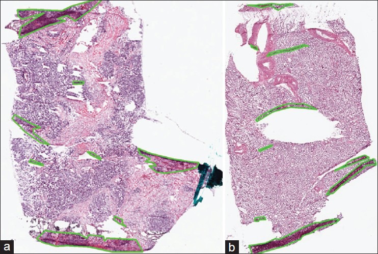
Manual annotation of tissue folds in whole-slide images from the cancer genome atlas. Tissue folds marked in WSIs of two types of carcinomas: (a) Ovarian serous adenocarcinoma and (b) kidney renal clear cell carcinoma

Tissue-Region Identification

Before detecting tissue folds in a WSI, we identify regions in the WSI that contain tissue. A typical TCGA WSI contains large white regions representing blank, tissue-less portions of the slide and some bluish-green regions representing pen marks used by pathologists to annotate the slide. These blank and pen-marked regions are not informative for cancer diagnosis, so we remove these regions from further consideration. For convenience, we represent the tissue, blank, and pen-marked regions as logical matrices A, W, and P, respectively, with dimensions equal to the WSI dimensions. The value of A, W, and P at a pixel location (x, y) is given by a(x, y), w(x, y), and p(x, y), respectively. We use hue (h), saturation(s), and intensity (i) (Hexcone model[9]) of the pixel (x, y) to determine w and p, given by w(x, y) = II[s(x, y) ≤ 0.1] and p(x, y) = II[(0.4 < h(x, y) < 0.7∩s(x, y) > 0.1) ∪i(x, y) < 0.1], where II (c) is an identity function that returns logical 1 if c is true. We morphologically clean the W and P masks to remove noisy regions. Finally, if a pixel is zero in both the W and P masks, then it is one in tissue mask A, given by a(x, y) =1-II{[w(x, y) ∪ p(x, y)]}. We use only tissue regions for fold detection. Figure 2 is an example result for the detection of tissue regions. In Figure 2b, we have painted the pen-marked and blank regions as gray and black, respectively.

Figure 2.

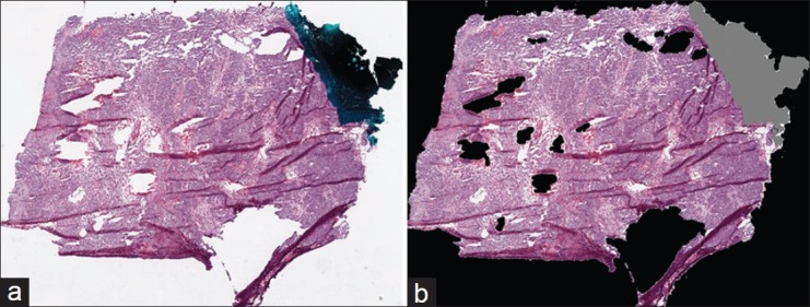
Tissue-region detection in a whole-slide image from the cancer genome atlas: (a) original RGB thumbnail and (b) painted thumbnail, in which pen-mark and blank regions are painted gray and black, respectively

Tissue-Fold Detection

Connectivity-Based Soft Threshold

We propose a novel method for detecting tissue folds in WSIs using color and connectivity properties of tissue structures. A WSI of a tissue-biopsy slide stained with H and E has three primary regions: Tissue structures (nuclei and cytoplasm), blank slide, and tissue folds. These regions differ in their color saturation and intensity properties: (1) Tissue folds are regions with multiple layers of stained tissue resulting in image regions with high saturation and low intensity,[6] (2) nuclear regions are stained blue-purple and have low intensity, and (3) cytoplasmic regions are stained pink and have high intensity. Therefore, we apply color saturation and intensity values to classify a pixel (x, y) into the tissue-fold region. We subtract the color intensity i(x, y) from color saturation s(x, y) for each pixel, resulting in a difference value d(x, y) = s(x, y) – i(x, y), where d(x, y) ∈[1 −1]. Typically, d(x, y) is high in tissue-fold regions, intermediate in nuclear regions, and low in cytoplasmic regions. If we threshold the difference image, D (including all pixels), with various thresholds in the range of negative one to one, t∈ {−1, −0.95,…,0,…,0.951}, then the following three patterns emerge: (1) At high thresholds, only a few connected objects (i.e., mostly tissue folds) are segmented; (2) at medium thresholds, a large number of connected objects (i.e., mostly tissue folds and nuclei) are segmented; and (3) at low thresholds, only a few large connected objects (i.e., tissue structures merged with cytoplasm) are segmented. Our goal is to find an optimal threshold that segments only tissue folds. However, we observed that this threshold varies because of variations in tissue samples, preparation sites, and acquisition systems. Thus, we hypothesize that an approximate tissue-fold threshold can be predicted based on object connectivity in a WSI. In Figure 3, we illustrate the following for a WSI: (1) the difference image, (2) manually annotated folds, (3) segmented binary images B(t) at various thresholds, and (4) the distribution of connected-object count C(t) using 8-connectivity at various thresholds. The peak of the distribution corresponds to the approximate threshold at which dark nuclear structures are segmented but not merged. We hypothesize that tissue folds can be detected by a threshold greater than the threshold corresponding to the peak, and this threshold is a function of connected-object count at the peak. Our hypothesis is based on an assumption that, for any dataset, tissue-fold objects are a small percentage of all connected objects at the peak. We can safely make this assumption because of the nature of tissue folds. Tissue-fold artifacts are caused by the folding of tissue slices when placed on a glass slide. Thus, folds are seldom randomly distributed over the whole-slide, which would lead to a large number of connected objects (greater than the number of nuclear objects). Even if a large portion of the image contains tissue folds, most tissue-fold pixels are likely to be connected within a small number of tissue-fold regions.

Figure 3.

Estimation of soft and hard thresholds for detecting tissue folds in the connectivity-based soft threshold method. An example ovarian serous adenocarcinoma whole-slide image (a) has multiple tissue folds detected by manual annotation as shown in a binary mask (b) a difference image (c) is calculated by subtracting intensity from saturation of every pixel in (a). The binary masks obtained by thresholding the difference image at three thresholds − 0.45 (d), − 0.3 (e), and − 0.05 (f) contain connected objects painted by pseudo-colors. The distribution (g) of the number of connected objects at various thresholds is used to calculate optimal thresholds. For parameters α = 0.64 and β = 0.34, the optimal thresholds are t_hard = − 0.15, and t_soft = − 0.2

The difference value, d(x, y), for tissue folds in a WSI varies within a range, especially in the area surrounding a strong tissue fold. Therefore, we propose to use two thresholds – hard, t_hard, and soft, t^soft, and a neighborhood criterion. Both thresholds are a function of connected-object count C(t) given by t_hard = T(α*max C(t)) and T(β*max C(t)), where T is a function of count defined by T(c) = max {t / C(t) ≥ c}. Based on these thresholds, we classify a pixel as a tissue fold if the following conditions are true: (1) It has a difference value, d(x, y), higher than the soft threshold and (2) it is in the 5 × 5 neighborhood of a pixel with a difference value greater than the hard threshold. Mathematically, this is given by

where b (t,x,y) = II(d (x,y)>t)

The soft threshold allows tissue-fold pixels in the neighborhood of strong tissue folds to have a lower difference value. The value of f(x, y) for all pixels generates a tissue-fold image, F. However, F may still have some small, noisy connected objects. We discard these noisy objects in the tissue-fold image using an adaptive area threshold equivalent to 5% of the area of a high-resolution tile in a WSI (i.e., 512 × 512 pixels).

The hard and soft thresholds depend on parameters α and β. Both tissue morphology and connectivity differ from one cancer endpoint to another cancer endpoint. Thus, we optimize α and β for each TCGA dataset. We optimize these parameters on a set of training images and then evaluate the selected parameters on a set of testing images. We split our annotated data (105 images for each cancer) into 50 pairs of training and testing sets using ten iterations of 5-fold cross-validation. For each cross-validation split, we select optimal parameters by maximizing the average adjusted Rand index (ARI) on the training set. The Rand index is a statistical measure that quantifies the similarity between two sets of data clusters. When applied to tissue-fold detection, the Rand index counts the number of agreements in pixel pairs between the detected tissue-fold pixels and the ground truth. For example, if both pixels in a pixel pair are part of the same class in the ground truth (i.e., either both pixels are tissue folds, or they are not), a pixel pair agrees with the ground truth if both pixels are detected as being in the same class (e.g., tissue folds). Alternatively, if both pixels in a pair are in different classes in the ground truth (i.e. one pixel is a tissue fold, and the other is not), the pair is not in agreement if both pixels are detected as being in the same class. The Rand index is the ratio of the number of agreeing pairs to the total number of pairs. To account for different class prevalence (i.e. different numbers of pixels in tissue-fold vs. non-tissue-fold regions), we use the ARI, which is a modification of the Rand index. For two classes, the ARI is given by

where m_g,p indicates the number of pixels designated as g in the ground truth and predicted to be p, where (g, p){fold, tissue}. For example, m_fold,tissue indicates the number of pixels designated as part of the tissue-fold regions in the ground truth, but is predicted to be part of non-tissue-fold regions. M is the total number of pixels; m_g,o = m_g,fold + m_g,tissue is the total number of pixels designated as g in the ground truth; and m_o,p = m_fold,p + m_tissue,p is the number of pixels predicted to be p. Because a segmented image can be perceived as a clustering of pixels into groups, the Rand index and its various forms are often used for image-segmentation evaluation.[10,11] We have chosen ARI for our evaluation because it is invariant to class prevalence. In most WSIs, tissue-fold regions are a small percent of the tissue region. Thus, errors in fold detection will not significantly affect a metric that is invariant to class prevalence. For example, accuracy calculates the number of pixels assigned to the correct class regardless of the class. Since there are usually more tissue pixels than tissue-fold pixels, methods that classify tissue pixels correctly may appear to perform well in terms of accuracy even if the methods compromise the performance of tissue-fold detection. In other words, metrics that do not account for prevalence tend to severely down-weight the sensitivity of tissue-fold detection.

We optimize α and β in the range of 0-1 with two levels of quantization: Coarse and fine. While optimizing, we allow only pairs in which α is greater than β so that t_hard is greater than t_soft. During coarse optimization, we vary the parameters with steps of 0.1 in the range of 0-1 and calculate the parameter pair, α_c and β_c, with the maximum ARI, averaged over all training samples. During fine optimization, we vary the parameters with steps of 0.01 in the range of α_c − 0.1 to α_c + 0.1 and β_c − 0.1 to β_c + 0.1. The two-level optimization speeds up the optimization process.

Clustering

As a comparison, we implement a clustering-based method for tissue-fold detection suggested by Palokangas et al.[6] This method has three steps: Preprocessing, segmentation, and discarding of extra objects. In our implementation, we first detect tissue regions in a WSI and then follow these three steps. First, we subtract smoothed and contrast-enhanced saturation Ŝ and intensity Î images of a WSI and calculate the difference image Second, we cluster the pixels of the difference image using k-means clustering and assign the cluster of pixels with center at the maximum difference value as tissue folds. Finally, we discard extra objects in the tissue-fold image using an adaptive area threshold equivalent to five percent of a tile area in the highest resolution of the WSI. For k-means clustering, we optimize the number of clusters, n, based on the change in the average sum of the difference (variance) over all clusters. We start optimization with n = 2 clusters and terminate at n = 6 clusters; we select a value of n for which the change in variance compared to the variance with n-1 clusters is less than one percent.

Soft Threshold

Instead of clustering the difference image, we can also find tissue folds by applying a soft and hard threshold, as done in the Proposed connectivity-based soft threshold (ConnSoftT) method. However, in the ConnSoftT method, we apply adaptive thresholds based on tissue connectivity after optimizing α and β. Alternatively, we can directly optimize the hard, H_T, and soft, S_T, thresholds for a dataset. Therefore, for comparison, we implement the direct-optimization version for soft thresholding by repeating all of the steps from the ConnSoftT method, excluding the connectivity-based analysis and optimization steps. After obtaining the difference image, D, we optimize H_T and S_T in the range of −1 to +1, with the condition that the hard threshold is greater than the soft threshold. Similar to the ConnSoftT method, we optimize the thresholds using two quantization levels (i.e., coarse with steps of 0.2 and fine with steps of 0.02), manually annotated training data, and the ARI performance metric. Finally, after thresholding the difference image, we discard noisy objects using an adaptive area threshold (the same threshold as in the ConnSoftT method).

Image Feature Extraction and Classification

We extract image features from the highest-resolution WSIs using piecewise analysis.[12] After dividing the WSIs into matrices of 512 × 512-pixel, non-overlapping tiles, we select tiles with greater than 50% tissue and less than 10% tissue folds. From each tile, we extract 461 quantitative image features capturing the texture, color, shape, and topological properties of a histopathological image.[12,13] Based on these features, we eliminate non-tumor (necrosis or stroma) tiles using a supervised tumor versus non-tumor classification model.[12] We then combine image features extracted from tumor tiles in all WSIs of each individual patient. The tile combination process consists of four methods depending on the type of feature being combined. The mean features (e.g., mean nuclear area) are combined using an average, weighted by the number of objects in each tile. The median features are combined by computing the median over all tiles. Similarly, the minimum and maximum features are computed using the minimum over all tiles and the maximum over all tiles, respectively. Finally, features that are standard deviations are computed using group standard deviation, which accounts for the number of objects in each tile. We develop binary – high versus low – grading models for OvCa and KiCa. To develop grading models, we apply classifiers based on discriminant analysis (i.e., linear, quadratic, spherical, and diagonal) and use minimum-redundancy, maximum-relevance feature selection.[14] We optimize the feature size within the range of one to twenty-five and we optimize classifier parameters using nested cross-validation.

RESULTS AND DISCUSSION

We compare the performance of the ConnSoftT, clustering (Clust), and soft threshold (SoftT) methods in detecting tissue folds. In addition, we study the effect of tissue folds on image features and cancer-grading models.

Comparison of ConnSoftT, Clust, and SoftT Methods for Detection of Tissue Folds

In this section, we discuss the performance of the ConnSoftT method and compare it to two other methods: Clust and SoftT. We test the methods on two OvCa and KiCa datasets, each with 105 images and manually annotated tissue folds. Using ten iterations of 5-fold cross-validation, we divide the datasets into 50 pairs of training and testing sets, in which each training set is used for optimizing models in the ConnSoftT and SoftT methods while the testing set is used to test all three methods. We assess the performance of detecting tissue folds using four metrics: (1) ARI, which was also used for model optimization, (2) the true positive rate (TPR), or sensitivity, (3) the true negative rate (TNR), or specificity, and (4) the average true rate (ATR) (i.e., the average of TPR and TNR). The average and standard deviation of performance metrics over 50 iterations of cross-validation on KiCa and OvCa images are listed in Tables 1 and 2, respectively. The best method should result in all metrics closer to one. A high TNR and a low TPR indicates that the method under-segments tissue folds while a low TNR and a high TPR indicate that the method over-segments. Therefore, the best method should have high ATR. From these tables, we can make several observations. First, compared to the other methods, the ConnSoftT method detects tissue folds more effectively because it has the highest ARI (0.50 in KiCa and 0.40 in OvCa) and ATR (0.77 in KiCa and 0.73 in OvCa). Second, based on TNR, TPR and ATR, the Clust method under-segments tissue folds (TNR is highest at 0.99 in KiCa and 0.98 in OvCa) while the SoftT method over-segments tissue folds (TPR is highest at 0.62 in KiCa and 0.57 in OvCa). The ConnSoftT method achieves a balance between the two methods (ATR is highest at 0.77 in KiCa and 0.73 in OvCa). Third, all three methods have lower TPR than TNR. TPR is more sensitive to faults in tissue-fold detection than TNR because the positive class (tissue-fold regions) has a lower prevalence than the negative class (non-tissue-fold regions). The difference in the prevalence is the main motivation for using ARI, which is adjusted for prevalence, for parameter optimization in the ConnSoftT and SoftT methods.

Table 1.

Tissue-fold detection performance in KiCa images

Table 2.

Tissue-fold detection performance in OvCa images

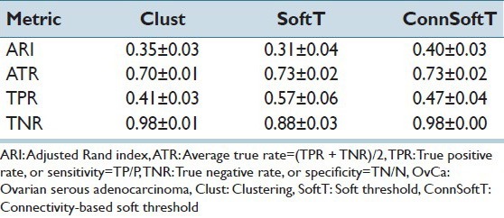
Figure 4 illustrates tissue-fold detection results for three WSIs using the three methods with the final model parameters. Since Clust is an unsupervised method, when it finds a cluster of pixels in a WSI with the highest difference value, it is not certain if this cluster represents tissue folds or if this cluster includes all of the tissue-fold pixels in the WSI. Figure 4 presents the results of this uncertainty. Figures 4c and h show that the Clust method under-segments, and Figure 4m shows that the Clust method over-segments. Although the SoftT method is supervised, because of the variations in the color properties of WSIs, fixed thresholds cannot successfully segment tissue folds in all WSIs. For example, Figures 4a and 4k depict over-segmentation using the SoftT method when WSIs are darker than the remaining set of images. In contrast, ConnSoftT is supervised and adapts to a WSI based on its tissue connectivity, which results in more effective tissue-fold detection regardless of variations across images within a dataset.

Figure 4.

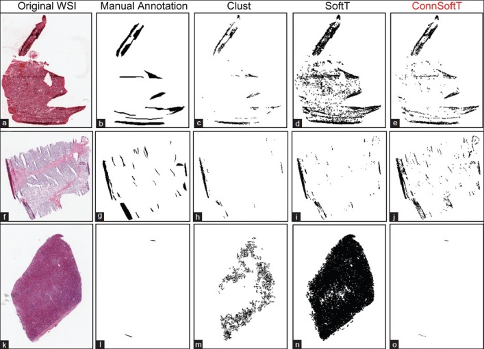
Comparison of the performance of the three tissue-fold detection methods: Clustering, Soft threshold, and Connectivity-based soft threshold. Tissue folds detected by the three methods: Clust (c, h, and m), SoftT (d, i, and n), and ConnSoftT (e, j, and o) for an ovarian serous adenocarcinoma whole-slide image (a) and two kidney clear cell carcinoma WSIs (f and k). If tissue folds in a WSI vary in color (a and f), the Clust method under segments. On the other hand, if a WSI has no tissue folds in (k), Clust over segments. Because of the fixed thresholding of the SoftT method, it over segments WSIs (a and k) with darker tissue regions and under segments WSIs (f) with lighter tissue folds

Parameter Optimization and Sensitivity Analysis

In this section, we conduct a sensitivity analysis on the parameters of the ConnSoftT and SoftT methods to show that (1) optimal parameters for both methods are robust with respect to the training samples for a specific cancer endpoint, but are sensitive to the cancer endpoint; (2) compared to the SoftT method, the ConnSoftT method is more adaptive and can better handle the large variations among images; and (3) the performance of the ConnSoftT method is robust to small variations in α and β.

Both the ConnSoftT and SoftT methods require two parameters (α and β for the ConnSoftT method; HT and ST for the SoftT method) that are optimized using a ground truth of training samples within 50 iterations of cross-validation. In Figure 5, we illustrate the frequency of parameter-pair selection using color maps. For both methods, the optimal parameters tend to be selected within a local area of the parameter space, which extends from −1 to 1 for H_T and S_T and from 0 to 1 for α and β. The average of selected parameter pairs during cross-validation [Table 3] closely resembles the parameters of the final models [Table 4], which were optimized using the complete set of 105 images. Low standard deviation in the selection of the parameter pairs during cross-validation and the similarity of average parameters to the final model parameters indicate that the selection of parameters (in both methods) is robust to variations in training samples for a cancer endpoint. However, the difference in the optimal parameters of the two cancer endpoints supports our hypothesis that the pair α and β should vary from one cancer endpoint to another because of differences in morphology between the endpoints.

Figure 5.

Optimal parameter selection in the Soft threshold (SoftT) and Connectivity-based soft threshold (ConnSoftT) methods. Heat map for the frequency of parameter-pair selection during 50 iterations (5-fold, 10 iterations) of cross-validation for kidney clear cell carcinoma (a and b) and ovarian serous adenocarcinoma (c and d) images. For the SoftT method, the hard and soft thresholds were optimized (a and c). For the ConnSoftT method, α and β were optimized (b and d). Note: In both heatmaps, the parameter space with no selection (zero frequency) has been cropped

Table 3.

Mean and sample deviation of selected parameters during cross-validation

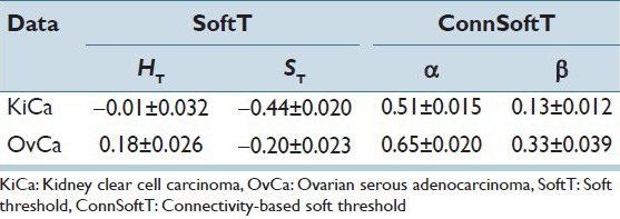
Table 4.

Parameters for final model estimated using the entire data set

For optimal segmentation of tissue folds, and because of the variations across images, hard and soft thresholds should adapt to each image within a cancer endpoint. In the ConnSoftT method, thresholds depend on parameters (α and β) and the connected-object function. The function adapts to each image to produce an optimal segmentation. For instance with the final α and β parameters [Table 4], soft and hard thresholds for 105 OvCa WSIs vary, but tend to fall within the ranges 0.0995 ± 0.2101 and −0.0162 ± 0.1981, respectively. Similarly, soft and hard thresholds for 105 KiCa WSIs tend to fall within the ranges −0.0724 ± 0.2234 and −0.2586 ± 0.2139, respectively. In contrast, the soft and hard thresholds are fixed in the SoftT method [Table 4]. Hence, in contrast to the SoftT method, the connectivity-based method adapts to each image.

Figure 6 illustrates the robustness of the ConnSoftT method to small variations in the α and β parameters. The heatmap illustrates average ARI for tissue-fold detection on the entire data set of 105 images using the allowable set of coarse parameters (α > β). The performance of the method is quite similar in the range of parameters selected during cross-validation (marked by the dashed rectangle). Thus, tissue-fold detection using the ConnSoftT method is robust to small changes in α and β.

Figure 6.

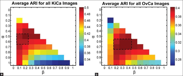
Sensitivity of Connectivity-based soft threshold method to parameter selection. Heat map for the average performance (adjusted Rand index) of tissue-fold detection using ConnSoftT method with different parameters. The average was calculated using the entire data set of 105 images for both kidney clear cell carcinoma (a) and ovarian serous adenocarcinoma (b). The performance of the method is quite similar in the range of parameters (marked by a dashed rectangle) selected during cross-validation [Figure 5], indicating that tissue-fold detection is not sensitive to small parameter changes

Effect of Tissue-Fold Elimination on Quantitative Image Features and Cancer Diagnosis

Previous studies have discussed the need for eliminating tissue-fold image artifacts before extracting image features and building diagnostic models. However, to the best of our knowledge, no published work investigates the effect of tissue folds on quantitative image features and cancer diagnosis. We identify image features changed by the presence of tissue folds using a rank-sum test of two lists of feature values in WSIs with and without tissue folds. If the P value for the test is < 2.1692e − 005 (i.e. a P value threshold of 0.01, adjusted for multiplicity by the Bonferroni method, 0.01/461), then this indicates that a feature changes (with statistical significance) in the presence of tissue folds. Figure 7 shows several image features changed by tissue folds. We found that 30 and 53 features changed as a result of the presence of tissue folds in OvCa and KiCa, respectively. Out of these features, most capture an extreme value or variation in a property such as the minimum averaged distance of a nucleus to its five neighbors and the standard deviation of nuclear area. Moreover, the presence of tissue folds increases the spread of most features. Hence, tissue-fold artifacts create outlier regions in a WSI. To investigate the effect of tissue folds on predictive grading models, we develop predictive models for kidney and ovarian cancer grading for WSIs using the features changed by tissue folds. We found that, without folds, these predictive models have higher area under the curve (AUC), as assessed with ten iterations of 5-fold cross-validation Table 5. The improvement in AUC is more prominent for the OvCa data set, which includes WSIs with a higher percent of tissue folds Figure 8. Therefore, we can conclude that the presence of tissue folds changes several quantitative image features. Consequently, after eliminating the tissue-fold regions in WSIs, prediction models based on these image features can more accurately classify WSIs into groups of high and low grade.

Figure 7.

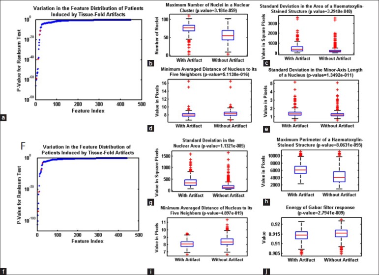
Effect of tissue-fold elimination on quantitative image features. Variation in quantitative image features in the whole-slide images of kidney clear cell carcinoma (KiCa) (a-e) and ovarian serous adenocarcinoma (OvCa) (f-k) samples in the presence of tissue folds. P values are calculated for all image features to identify features most affected by tissue-folds (ordered by P value of the rank-sum test) for both KiCa (a) and OvCa (f). With the presence of tissue folds, 30 and 53 image features statistically changed in KiCa and OvCA, respectively. Using box-plots, we illustrate the distribution of certain features (highlighted in red) changed by tissue folds

Table 5.

AUC of predictive grading models with and without tissue folds

Figure 8.

The percent of tissue folds in whole-slide images from the cancer genome atlas. The value on the y-axis represents the percent of tissue tiles eliminated because of tissue folds in samples per patient. Samples for patients with ovarian carcinoma have more tissue folds than those for patients with kidney carcinoma

CONCLUSION

Imaging informatics methods strive to develop automated, quantitative models for cancer prediction in histopathological WSIs. To insure the robustness of these models, we have to control the quality of WSIs by detecting and eliminating artifacts. We developed a novel method for detecting tissue-fold artifacts from low-resolution WSIs by estimating adaptive soft and hard thresholds based on tissue connectivity in the saturation and intensity color space. Compared to two other methods, our method performed better based on the ARI and the average true detection rate. We illustrated the importance of tissue-fold elimination in an informatics pipeline by highlighting quantitative image features sensitive to tissue folds and using these image features to develop ovarian and kidney carcinoma predictive grading models for WSIs. We found that the elimination of tissue folds from WSIs improved the image-based prediction of ovarian and kidney cancer grades.

REFERENCES

- 1.Pantanowitz L, Valenstein PN, Evans AJ, Kaplan KJ, Pfeifer JD, Wilbur DC, et al. Review of the current state of whole slide imaging in pathology. J Pathol Inform. 2011;2:36. doi: 10.4103/2153-3539.83746. [DOI] [PMC free article] [PubMed] [Google Scholar]
- 2.Sadimin ET, Foran DJ. Pathology imaging informatics for clinical practice and investigative and translational research. N Am J Med Sci (Boston) 2012;5:103–9. doi: 10.7156/v5i2p103. [DOI] [PMC free article] [PubMed] [Google Scholar]
- 3.Chang H, Fontenay GV, Han J, Cong G, Baehner FL, Gray JW, et al. Morphometic analysis of TCGA glioblastoma multiforme. BMC Bioinformatics. 2011;12:484. doi: 10.1186/1471-2105-12-484. [DOI] [PMC free article] [PubMed] [Google Scholar]
- 4.Cooper LA, Kong J, Gutman DA, Wang F, Gao J, Appin C, et al. Integrated morphologic analysis for the identification and characterization of disease subtypes. J Am Med Inform Assoc. 2012;19:317–23. doi: 10.1136/amiajnl-2011-000700. [DOI] [PMC free article] [PubMed] [Google Scholar]
- 5.Cancer Genome Atlas Research Network. Comprehensive genomic characterization defines human glioblastoma genes and core pathways. Nature. 2008;455:1061–8. doi: 10.1038/nature07385. [DOI] [PMC free article] [PubMed] [Google Scholar]
- 6.Palokangas S, Selinummi J, Yli-Harja O. Segmentation of folds in tissue section images. Conf Proc IEEE Eng Med Biol Soc. 2007;2007:5642–5. doi: 10.1109/IEMBS.2007.4353626. [DOI] [PubMed] [Google Scholar]
- 7.Bautista PA, Yagi Y. Detection of tissue folds in whole slide images. Conf Proc IEEE Eng Med Biol Soc. 2009;2009:3669–72. doi: 10.1109/IEMBS.2009.5334529. [DOI] [PubMed] [Google Scholar]
- 8.Bautista PA, Yagi Y. Improving the visualization and detection of tissue folds in whole slide images through color enhancement. J Pathol Inform. 2010;1:25. doi: 10.4103/2153-3539.73320. [DOI] [PMC free article] [PubMed] [Google Scholar]
- 9.Smith AR. In: ACM Siggraph Computer Graphics. ACM New York, NY, USA: ACM; 1978. Color gamut transform pairs; pp. 12–9. [Google Scholar]
- 10.Unnikrishnan R, Pantofaru C, Hebert M. Toward objective evaluation of image segmentation algorithms. IEEE Trans Pattern Anal Mach Intell. 2007;29:929–44. doi: 10.1109/TPAMI.2007.1046. [DOI] [PubMed] [Google Scholar]
- 11.Jiang X, Marti C, Irniger C, Bunke H. Distance measures for image segmentation evaluation. EURASIP J Appl Signal Processing. 2006;2006:209. [Google Scholar]
- 12.Kothari S, Phan JH, Osunkoya AO, Wang MD. In: Proceedings of the 3rd ACM Conference on Bioinformatics, Computational Biology and Biomedicine. ACM New York, NY, USA: ACM; 2012. Biological interpretation f morphological patterns in histopathological whole-slide images; pp. 218–25. [DOI] [PMC free article] [PubMed] [Google Scholar]
- 13.Kothari S, Phan JH, Young AN, Wang MD. IEEE Computer Society. Washington, DC, USA: IEEE; 2011. Histological image feature mining reveals emergent diagnostic properties for renal cancer. BIBM ‘11 Proceedings of the 2011 IEEE International Conference on Bioinformatics and Biomedicine; pp. 422–5. [DOI] [PMC free article] [PubMed] [Google Scholar]
- 14.Ding C, Peng H. Minimum redundancy feature selection from microarray gene expression data. J Bioinform Comput Biol. 2005;3:185–205. doi: 10.1142/s0219720005001004. [DOI] [PubMed] [Google Scholar]