Binding constants of membrane-anchored receptors and ligands depend strongly on the nanoscale roughness of membranes

Abstract

Cell adhesion and the adhesion of vesicles to the membranes of cells or organelles are pivotal for immune responses, tissue formation, and cell signaling. The adhesion processes depend sensitively on the binding constant of the membrane-anchored receptor and ligand proteins that mediate adhesion, but this constant is difficult to measure in experiments. We have investigated the binding of membrane-anchored receptor and ligand proteins with molecular dynamics simulations. We find that the binding constant of the anchored proteins strongly decreases with the membrane roughness caused by thermally excited membrane shape fluctuations on nanoscales. We present a theory that explains the roughness dependence of the binding constant for the anchored proteins from membrane confinement and that relates this constant to the binding constant of soluble proteins without membrane anchors. Because the binding constant of soluble proteins is readily accessible in experiments, our results provide a useful route to compute the binding constant of membrane-anchored receptor and ligand proteins.

A central problem in cell adhesion is to quantify the binding affinity of the membrane-anchored receptor and ligand proteins that cause adhesion (1–4). The distinction of “self” and “foreign” in cell-mediated immune responses, for example, depends on subtle affinity differences between receptor and ligand proteins anchored on the surfaces of apposing cells (5). The binding affinity of anchored receptor and ligand proteins, which are restricted to the two-dimensional (2D) membrane environment, is typically described by the binding equilibrium constant K_2D of the proteins. Because K_2D is difficult to measure in experiments, it is often estimated from the binding constant K_3D of soluble variants of the receptors and ligands that lack the membrane anchors and are free to diffuse in three dimensions (3D). Standard approaches are based on the relation suggested by Bell et al. (6), where l_c is a characteristic length that reflects the different units of area and volume for K_2D and K_3D, respectively. However, different methods to measure the binding equilibrium constant of membrane-anchored proteins have led to values of K_2D and associated values of l_c that differ by several orders of magnitude (7). In contrast to the standard approaches, the simulation data and theory presented here indicate that the relation between K_2D and K_3D involves three different length scales, and that the most important of these length scales is the membrane roughness resulting from shape fluctuations on nanoscales. Because the membrane roughness depends on the concentration of the receptor–ligand bonds that constrain the shape fluctuations, our results help to understand differences in K_2D values from different experiments.

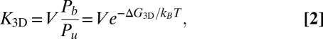
In this article, we report simulations of biomembrane adhesion with a molecular model of lipids and proteins (Fig. 1A). We systematically vary the size of the membranes and the numbers of receptors and ligands and determine the binding constant K_2D and the on- and off-rate constants k_on and k_off of the membrane-anchored receptors and ligands for these different systems with high precision from thousands of binding and unbinding events observed in our molecular dynamics simulations. Our largest apposing membranes are composed of 9,838 lipid molecules each and include 15 membrane-anchored receptors and ligands, respectively (Fig. 1C), whereas the smallest membranes contain 296 lipids and single receptor and ligand molecules. In addition, we determine the binding constant K_3D and the on- and off-rate constants of soluble variants of our receptors and ligands without membrane anchors.

Fig. 1.

(A) Coarse-grained structures of a lipid molecule and of a membrane-anchored receptor or ligand. The hydrophilic head group of a lipid molecule consists of three beads (dark gray), and the two hydrophobic chains are composed of four beads each (light gray) (8). The membrane-anchored receptors and ligands consist of 84 beads arranged in a cylindrical shape and have hydrophobic anchors that are embedded in the lipid bilayer and mimic the transmembrane segments of membrane proteins. The transmembrane anchor of a receptor or ligand molecule is composed of four layers of hydrophobic lipid-chain–like beads (yellow) in between two layers of lipid-head–like beads (blue). The interaction domain of the receptor and ligand molecules consists of six layers of hydrophilic beads (red), with an interaction bead or “binding site” located in the center of the top layer of beads (black). (B) Simulation snapshot of two apposing membranes bound together by a single anchored receptor and ligand molecule. For clarity, the interaction domain of the receptor is shown in red and the interaction domain of the ligand in green. Each membrane here has an area of 30 × 30 nm². (C) Simulation snapshot of two apposing membranes of area 80 × 80 nm² interacting via 15 anchored receptor and 15 ligand molecules. The water beads are not displayed in these snapshots.

We find that K_2D is not a constant, but depends strongly on the relative roughness ξ_⊥ of the apposing membranes. The relative membrane roughness is the local standard deviation (SD) of the membranes from their average separation due to thermally excited shape fluctuations. The relative roughness varies with the concentration of the bound receptor–ligand complexes because the complexes constrain membrane shape fluctuations. At the optimal average membrane separation for receptor–ligand binding, the binding constant K_2D is inversely proportional to the membrane roughness for roughnesses larger than about 0.5 nm and, thus, even for roughnesses that are significantly smaller than the membrane thickness.

To understand the roughness dependence of K_2D and the relation of K_2D to the binding equilibrium constant K_3D of soluble receptors and ligands without membrane anchors, we have developed a general theory in which the binding free energy of the receptor–ligand complexes is decomposed into enthalpic and entropic terms. We find that the roughness dependence of K_2D can be fully understood from the entropy loss of the membranes upon receptor–ligand binding. The theory is in good quantitative agreement with our simulation results and provides a unique route to calculate K_2D from experimental values for K_3D. In addition to the membrane roughness, our theory includes two characteristic lengths of the receptor–ligand complexes, which reflect variations in the overall extension and in the binding site of the complexes.

Results

Binding Constant K_2D of Membrane-Anchored Receptors and Ligands.

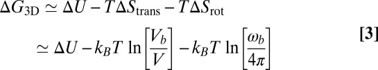
In our molecular dynamics simulations of biomembrane adhesion, the membranes are confined within a rectangular simulation box with periodic boundary conditions of size . Whereas the box extension L_z in the direction perpendicular to the membranes has the same value in all simulations, the extensions are varied to simulate different membrane sizes (Fig. 1 B and C). Binding events of the receptor and ligand proteins in our simulations can be clearly identified from the distance between the binding sites of the proteins (Fig. 2). The binding equilibrium constant K_2D of the anchored receptor and ligand proteins can then be calculated from the total dwell times in the bound and unbound states of the proteins observed in our simulations (Model and Methods).

Fig. 2.

Distance r between the binding sites of a single membrane-anchored receptor and ligand for a short time interval of a simulation with two apposing membranes of area 30 × 30 nm² as in Fig. 1B. Bound states of the receptor and ligand can be clearly identified from time segments in which the distance r between the centers of the binding sites exhibits small fluctuations around the value nm at which the minimum of the binding potential is located. In this example, the receptor and ligand bind twice and unbind twice.

The binding equilibrium constant and binding kinetics of membrane-anchored receptors and ligands depend on the distance between the two apposing membranes because receptor–ligand complexes cannot form if the two membranes are too far apart or too close. In Fig. 3, the binding constant K_2D of a single anchored receptor and a single anchored ligand molecule is shown as a function of the average membrane separation , which is kept constant in our simulations. In these simulations, the number of lipids is adjusted such that the membrane tension vanishes (8). For both membrane sizes and 30 × 30 nm², the binding constant K_2D is maximal at an average membrane separation close to the length of the receptor–ligand complexes. 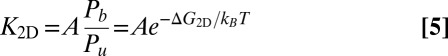In the following, we will focus on the average membrane separation at which K_2D is maximal because maxima in K_2D correspond to minima of the free-energy difference between the bound and unbound state of the membranes (Eq. 5). In a situation in which the membrane separation is not constrained, which is the typical situation in experiments, the membranes thus will “choose” the “optimal” average membrane separation . Within numerical accuracy, the optimal average membrane separation obtained from our simulations does not depend on the membrane size.

Fig. 3.

Binding constant K_2D as a function of the average membrane separation from simulations with membrane area (upper) and 30 × 30 nm² (lower) and a single membrane-anchored receptor and ligand pair. The dashed lines are guides for the eye.

In Fig. 3, the binding constants for the larger membrane area are significantly smaller than the binding constants for the membrane area . These differences in the binding constants for different membrane sizes can be understood from the shape fluctuations of the membranes. A characteristic measure for the strength of the fluctuations is the relative roughness of the two membranes, which is the SD of the local separation l_i of the membranes from the average separation where 〈…〉 denotes the thermodynamic average. To calculate the roughness ξ_⊥, we divide the x-y plane of our simulation box, which is on average parallel to the membranes, into patches i of size 2 × 2 nm², and determine the local separation l_i of two apposing patches from the separation of the membrane midplanes. In Fig. 4, the binding constants K_2D from different membrane systems are shown as a function of the membrane roughness ξ_⊥ at the optimal average membrane separation . The binding constant K_2D of the membrane-anchored receptors and ligands clearly decreases with the relative roughness ξ_⊥ of the membranes. The data shown in Fig. 4 are from simulations of membrane systems that differ in membrane area, number of receptors and ligands, membrane tension, or membrane potential. The dark blue data points in Fig. 4 are from simulations with tensionless membranes and a single receptor and ligand. The different values for K_2D and ξ_⊥ in these simulations result from different membrane sizes. The arrows in Fig. 4 indicate the two points that correspond to the two maxima of Fig. 3 for the membrane sizes 14 × 14 nm² and 30 × 30 nm². The roughness for the membrane area 30 × 30 nm² is about a factor 2 larger than the roughness for the membrane area 14 × 14 nm², whereas the K_2D value at the optimal separation is about a factor 2 smaller for the membrane area 30 × 30 nm². The membrane roughness in our simulations depends on the size of the membranes because the periodic boundaries of the simulation box suppress membrane shape fluctuations with wavelength larger than , where is the linear membrane size. The purple data points in Fig. 4 are from simulations with eight receptors and eight ligands and a membrane area of nm², and the brown data points from simulations with 15 receptors and 15 ligands and membrane area 80 × 80 nm². The different values for K_2D and ξ_⊥ in these simulations with tensionless membranes are for states with different numbers n of receptor–ligand bonds. These states exhibit different membrane roughnesses, as the receptor–ligand bonds constrain the membrane fluctuations (see Model and Methods for details). The three light blue data points are from simulations with positive (left point) or negative (two right points) membrane tension for the area 14 × 14 nm². Positive tension stretches the membranes and decreases the roughness, whereas negative tension compresses the membranes and increases the roughness. To extend the roughness range to smaller values, we have also performed simulations in which the membrane fluctuations are confined by membrane potentials (red points; see SI Text for details). In experiments, such a situation occurs for membranes bound to apposing surfaces as, for example, in the surface force apparatus (9, 10).

Fig. 4.

Binding constant K_2D at the optimal membrane separation for receptor–ligand binding as a function of the relative roughness ξ_⊥ of the two apposing membranes caused by thermally excited membrane shape fluctuations. The dark blue data points are from simulations with single membrane-anchored receptor and ligand molecules and tensionless membranes of area A = 14 × 14, 18 × 18, 22 × 22, 26 × 26, and 30 × 30 nm² (from left to right). The arrows indicate the two points that correspond to the maxima of Fig. 3 for the area 14 × 14 nm² (left arrow) and 30 × 30 nm² (right arrow). The light blue data points are from simulations with area 14 × 14 nm² and membrane tension 1.68 ± 0.01, −1.02 ± 0.02, and −1.50 ± 0.01 k_BT/nm² (from left to right). The red data points are from simulations with membrane area 14 × 14 nm² and confining potentials for head beads of the two distal monolayers of the membranes (see SI Text for details). The five purple data points are from simulations with eight receptor and eight ligand molecules and area 40 × 40 nm² of the two membranes, for the five binding reactions (from right to left), where n is the number of formed receptor–ligand complexes. The six brown data points result from simulations with 15 receptors and 15 ligands and membrane area 80 × 80 nm² (Fig. 1C), for the six binding reactions (from right to left). The dashed and full lines represent two fits to the data using the value for the binding constant of soluble receptors and ligands obtained from separate simulations. The dashed line is obtained from a least-square fit of the data points with roughness values larger than 0.5 nm to the functional form , which leads to as in Eq. 1. The full line is obtained from a least-square fit of all data points to the functional form given by Eq. 9. This fit leads to and .

The fact that all data points of Fig. 4 collapse onto a single curve indicates that the relative membrane roughness ξ_⊥ determines K_2D irrespective of whether the size of ξ_⊥ is controlled by the membrane area, the concentration of the receptor–ligand complexes, the membrane tension, or confining membrane potentials. For roughnesses larger than about 0.5 nm, this curve can be well fitted by the inverse proportionality relation

between the binding constant K_2D of the anchored receptors and ligands and the relative membrane roughness ξ_⊥ (see dashed line in Fig. 4). Here, K_3D is the binding constant of our soluble receptors and ligands without membrane anchors, which we have determined from simulations in water (see SI Text for details). The inverse proportionality between K_2D and the relative membrane roughness ξ_⊥ for sufficiently large roughnesses and the deviations from this proportionality for smaller roughness can be understood from a general theory for K_2D and K_3D derived in the next section.

A General Relation Between K_2D and K_3D.

We first focus on K_3D and consider a single soluble receptor and a single soluble ligand in a volume V. The two molecules are bound with equilibrium probability P_b, and unbound with probability P_u. Detailed balance implies , where and are the transition rates between the bound and unbound state of the molecules. Because of , we have

where is the binding free energy—that is, the free-energy difference between the bound and unbound state. We now consider the receptor and ligand as rigid rods with translational and rotational degrees of freedom. Following a standard approach in which the binding free energy is expanded around its minimum (11, 12), we obtain (see SI Text for details)

with the binding enthalpy ΔU and the loss and in translational and rotational entropy upon binding. Here, V_b is the translational phase space volume of the bound receptor relative to the ligand in the complex, and ω_b is the rotational phase space volume of the bound receptor relative to the ligand. In the unbound state, the rod-like receptor and ligand rotate freely with rotational phase space volume 4π. Eqs. 2 and 3 lead to the general result

for the binding constant of soluble receptor and ligand molecules.

In analogy to the soluble molecules, we now consider a single pair of membrane-anchored receptor and ligand molecules in two apposing membranes of area A. The transition rates between the bound and unbound state of the molecules are 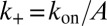and (Model and Methods). The detailed balance condition 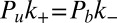and the definition 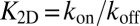then lead to

with the free-energy difference between the bound and unbound state. The free-energy difference can be decomposed as (see SI Text for details)

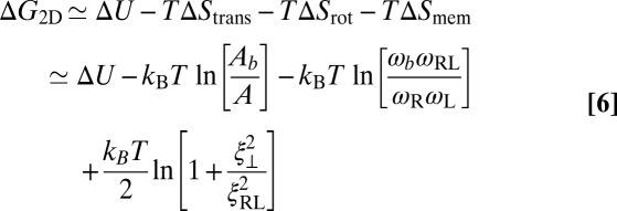with the translational and rotational entropy loss and of the receptor and ligand, and the entropy loss of the membranes upon bond formation. Here, A_b is the translational phase space area of the bound receptor relative to the ligand in the two directions parallel to the membranes, ω_R and ω_L are the rotational phase space volumes of the unbound membrane-anchored receptor and ligand molecules relative to the membranes, and ω_RL is the rotational phase space volume of a bound receptor or bound ligand relative to the membranes. 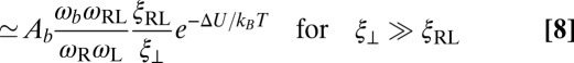The entropy loss of the membranes is obtained from exact results for a local harmonic constraint that restricts membrane shape fluctuations (13). This entropy loss depends on the relative roughness ξ_⊥ of the membranes and on a characteristic length ξ_RL that reflects intrinsic variations in the extension of the receptor–ligand complex in the direction perpendicular to the membranes, which result mainly from variations in the binding distance and anchoring angles of the molecules. Eqs. 5 and 6 lead to the general result

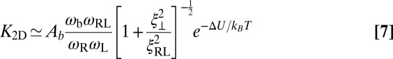
for the binding constant of the membrane-anchored receptors and ligands.

Finally, from a combination of Eqs. 4, 7, and 8, we obtain the general relation

between the binding equilibrium constant of the membrane-anchored molecules and the binding constant of their soluble counterparts without membrane anchors. We have assumed here that the binding interface of the membrane-anchored receptors and ligands is identical with the binding interface of their soluble counterparts (4), which implies that the binding enthalpy ΔU and the rational phase space volume ω_b of the bound receptor relative to the ligand are the same for both types of receptors and ligands. According to Eqs. 9 and 10, the ratio of the binding constants depends (i) on the membrane roughness ξ_⊥, (ii) on two characteristic lengths ξ_b and ξ_RL of the receptor–ligand complexes, and (iii) on the rotational phase space volumes , , and of the bound and unbound membrane-anchored receptors and ligands. The characteristic length ξ_b of the receptor–ligand complexes is defined as and can be calculated from the SD of the distance between the binding sites in the direction parallel to the receptor–ligand complex, as V_b is the translational phase space volume of the bound complex and A_b the translational phase space area in the two directions perpendicular to the complex, and parallel to the membranes (see SI Text for details). We obtain the value for our receptor–ligand complexes. The characteristic length ξ_RL can be determined from a comparison with our simulation results for K_2D at the optimal membrane separation, which leads to the estimate (see full line in Fig. 4). The rotational phase space volumes , , and can be calculated from the angular distributions of the receptors and ligands relative to the membranes. We obtain the values for our unbound receptors and ligands, and for bound receptors or bound ligands. From these values and the values for the characteristic lengths ξ_b and ξ_RL of the receptor–ligand complexes given above, we obtain the estimate for the numerical prefactor in Eqs. 9 and 10, which is consistent with the values obtained from fits to our simulation results for K_2D at the optimal membrane separation (see Eq. 1 and caption of Fig. 4).

On- and Off-Rate Constants.

Because K_2D can be expressed as the ratio of on- and off-rate constants k_on and k_off of the membrane-anchored receptors and ligands, an interesting question is whether the decrease of K_2D results from a decrease of k_on or an increase of k_off with the roughness, or both. We find that both k_on and k_off contribute to the roughness-dependence of K_2D, at least for the range of roughnesses accessible in our simulations (Fig. 5).

Fig. 5.

(A) On-rate constants k_on and (B) off-rates k_off of membrane-anchored receptors and ligands as a function of the relative membrane roughness ξ_⊥ from the same simulations as in Fig. 4.

For the soluble receptors and ligands without membrane anchors, we obtain the off-rate , which is about three to seven times larger than the off-rates obtained for the membrane-anchored receptor–ligand complexes. This finding is in agreement with experimental results for the binding of T-cell receptors to MHC-peptide ligands. The off-rates of soluble variants of these receptors and ligands without membrane anchors have been found to be slightly larger than the off-rates of the membrane-anchored receptors and ligands if the cytoskeleton of the cells is disrupted (14). In these experiments, the fluctuations of the cell membranes are governed by the membrane elasticity, as in our simulations. In experiments with intact cytoskeleton, the off-rates of membrane-anchored T-cell receptors and MHC-peptide ligands are larger than the off-rates of their soluble counterparts, presumably due to ATP-driven cytoskeletal forces acting on the membranes and receptor–ligand complexes (14–16).

Discussion and Conclusions

We have determined both the apparent binding constant K_2D of membrane-anchored receptors and ligands and the binding constant K_3D of soluble receptors and ligands with coarse-grained molecular dynamics simulations. In addition, we have developed a general theory for these binding constants that is in quantitative agreement with our simulation results. We find that K_2D is not a constant, but depends strongly on the membrane roughness ξ_⊥ from nanoscale shape fluctuations. In our general theory, the roughness dependence of K_2D is traced back to the entropy loss of the membranes upon the formation of a receptor–ligand complex. Our general relations between K_2D, K_3D, and the relative membrane roughness ξ_⊥ hold for any membrane system in which the anchored proteins are rather rigid and do not oligomerize or aggregate. The optimal membrane separation of about 15 nm for our receptor–ligand complexes is close to the length of complexes of, for example, the T-cell receptor or the protein CD2 (1, 17). The concentrations of our anchored receptors and ligands between 2,000 and 5,000 molecules per μm² are somewhat larger than typical concentrations of these proteins (1, 14, 17). In our simulations, we also used relatively large on- and off-rates to ensure an efficient sampling of binding and unbinding events. Therefore, the kinetics of these events is strongly enhanced compared with protein binding events in experiments. It is important to note, however, that our main results for the ratio of the binding constants are independent of the numerical values of the rate constants. These main results are (i) that is inversely proportional to the membrane roughness ξ_⊥ for roughnesses large compared with the characteristic length ξ_RL of the anchored receptor–ligand complexes (Eqs. 1 and 10) and (ii) that the prefactor of this inverse proportionality depends only on the molecular geometry of the receptor–ligand complex (Eq. 10). To illustrate that does not depend on the rate constants, we have performed additional simulations in which the binding energy of our receptors and ligands is increased by 25%. This increase in the binding energy increases both K_2D and K_3D by a factor 3.4 due to decreased off-rates, but does not change the ratio (see SI Text for details).

The roughness-dependence of K_2D leads to unusual laws of mass action for the binding of membrane-anchored receptor and ligand molecules. Membrane adhesion zones are typically large compared with the average distance of about between neighboring receptor–ligand bonds. Because the bonds constrain the membrane shape fluctuations, the average bond distance is proportional to the relative roughness ξ_⊥ of the membranes, which leads to the relation (18)

between the roughness ξ_⊥ and the concentration [RL] of receptor–ligand bonds. From Eq. 11 and the inverse proportionality of the binding constant and the relative roughness ξ_⊥ (Eq. 1), we obtain the quadratic relation

between the bond concentration [RL] and the concentrations [R] and [L] of the unbound receptors and ligands, which corroborates previous results from an elasticity model of biomembrane adhesion (19). This quadratic law of mass action indicates a cooperative binding of membrane-anchored receptors and ligands.

Model and Methods

Simulations.

Coarse-grained molecular dynamics simulations have been widely used to investigate the self-assembly (8, 20–22) and fusion (23–26) of membranes as well as the diffusion (27, 28) and aggregation (29) of membrane proteins. We have performed simulations with dissipative particle dynamics (30–32), a coarse-grained molecular dynamics technique that explicitly includes water. Our simulations of biomembrane adhesion include water beads, lipid molecules, and membrane receptors and ligands (Fig. 1). The lipid molecules consist of three hydrophilic head beads and two hydrophobic chains with four beads each, which are held together by harmonic potentials between adjacent beads and stiffened by bending potentials between three consecutive beads (8, 25, 26, 33). The membrane-anchored receptor and ligand molecules are composed of 84 beads that are arranged in a cylindrical shape of 12 hydrophobic or hydrophilic layers of seven beads each (Fig. 1A). Harmonic potentials between nearest and next-nearest neighbor beads lead to a rather stiff shape of the receptors and ligands. The specific binding of receptors and ligands is modeled via a distance- and angle-dependent attraction between two interaction beads that are located in the center of the top layers of beads (Fig. 1A). All other pairs of beads of the receptors, ligands, lipids, and water softly repel each other with a strength that depends on the bead types (see SI Text for details). In addition, we simulate the binding of soluble receptors and ligands in water. These soluble receptors and ligands lack the hydrophobic transmembrane anchor, but are otherwise identical with the membrane-anchored receptors and ligands.

Analysis of Binding Kinetics.

Binding and unbinding events of receptor and ligand molecules in our simulations can be identified from the distance between the binding sites of these molecules (Fig. 2). To distinguish binding and unbinding events from distance fluctuations in the bound and unbound state, we use two distance thresholds to define these events. A binding event is defined to occur when the distance r between the binding sites of a receptor and ligand falls below the binding threshold . An unbinding event is defined to occur when the binding-site distance of a bound receptor–ligand pair exceeds the unbinding threshold , which is well beyond the range of fluctuations in the bound state. The values for K_2D and K_3D and the relative values of the on- and off-rate constants of the receptors and ligands obtained from our analysis do not depend on the precise values of these thresholds.

The binding and unbinding events divide our simulation trajectories into different states with different numbers of bound receptor–ligand complexes. In our simulations with a single receptor and ligand molecule, we have two states: the unbound state of the molecules and the bound state with a single receptor–ligand complex. In our simulations with N_R receptors and N_L ligands, we have N + 1 states where is the maximum number of bound complexes. Our simulation trajectories thus can be mapped to a Markov model:

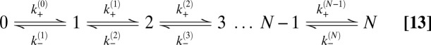with transition rates and between the states that are related to the binding and unbinding rate constants and of the receptors and ligands. The binding rate of an individual unbound receptor in state n is proportional to the concentration of unbound ligands and proportional to the rate constant for the formation of a bond in state n, where A is the area of the membranes. Because we have unbound receptors, the rate for a transition from state n to state n + 1 is:

for n < N. The rate for a transition from state n to n − 1 is:

for n > 0 because there are n bonds that may each break with rate . The binding constant is defined as:

The on- and off-rate constants can be determined from the observed numbers of transitions between the states and from the overall dwell times in the states. The binding and unbinding events divide the simulation trajectories into time windows i of length t_i in state n_i, which are followed by a transition into state n_i + s_i, where s_i is either 1 or −1. The probability for staying for a dwell time t_i in state n_i is with (SI Text). 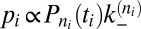The probability of time window i with its observed transition then is for and for . The likelihood function is the probability for the whole trajectory—that is:

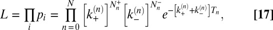where is the total number of transitions from n to n + 1, the total number of transitions from n to n − 1, and T_n the total dwell time in state n.

Maximizing L with respect to the binding and unbinding rate constants and of Eqs. 14 and 15 leads to the maximum likelihood estimators for the rate constants:

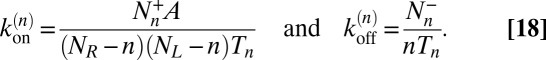Our estimator for the binding constant defined in Eq. 16 then is:

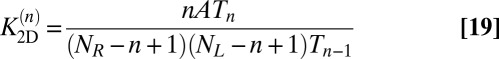
because the transition numbers and are identical in equilibrium. For our simulations with a single receptor and a single ligand, the maximum-likelihood estimators for the on- and off-rate constants thus are and , and the estimator for the binding constant is . For large numbers N_R and N_L of receptors and ligands and states with receptor–ligand bonds where is the average number of bonds, Eq. 19 is equivalent to with , , and as we then have and .

References

- 1.Dustin ML, Ferguson LM, Chan PY, Springer TA, Golan DE. Visualization of CD2 interaction with LFA-3 and determination of the two-dimensional dissociation constant for adhesion receptors in a contact area. J Cell Biol. 1996;132(3):465–474. doi: 10.1083/jcb.132.3.465. [DOI] [PMC free article] [PubMed] [Google Scholar]
- 2.Zhu D-M, Dustin ML, Cairo CW, Golan DE. Analysis of two-dimensional dissociation constant of laterally mobile cell adhesion molecules. Biophys J. 2007;92(3):1022–1034. doi: 10.1529/biophysj.106.089649. [DOI] [PMC free article] [PubMed] [Google Scholar]
- 3.Leckband D, Sivasankar S. Cadherin recognition and adhesion. Curr Opin Cell Biol. 2012;24(5):620–627. doi: 10.1016/j.ceb.2012.05.014. [DOI] [PMC free article] [PubMed] [Google Scholar]
- 4.Wu Y, Vendome J, Shapiro L, Ben-Shaul A, Honig B. Transforming binding affinities from three dimensions to two with application to cadherin clustering. Nature. 2011;475(7357):510–513. doi: 10.1038/nature10183. [DOI] [PMC free article] [PubMed] [Google Scholar]
- 5.Alberts B, et al. Molecular Biology of the Cell. New York: Garland Science; 2008. [Google Scholar]
- 6.Bell GI, Dembo M, Bongrand P. Cell adhesion. Competition between nonspecific repulsion and specific bonding. Biophys J. 1984;45(6):1051–1064. doi: 10.1016/S0006-3495(84)84252-6. [DOI] [PMC free article] [PubMed] [Google Scholar]
- 7.Dustin ML, Bromley SK, Davis MM, Zhu C. Identification of self through two-dimensional chemistry and synapses. Annu Rev Cell Dev Biol. 2001;17:133–157. doi: 10.1146/annurev.cellbio.17.1.133. [DOI] [PubMed] [Google Scholar]
- 8.Goetz R, Lipowsky R. Computer simulations of bilayer membranes: Self-assembly and interfacial tension. J Chem Phys. 1998;108(17):7397–7409. [Google Scholar]
- 9.Israelachvili JN. Intermolecular and surface forces. 1992. (Academic Press, Waltham, MA), 2nd Ed.
- 10.Bayas MV, Kearney A, Avramovic A, van der Merwe PA, Leckband DE. Impact of salt bridges on the equilibrium binding and adhesion of human CD2 and CD58. J Biol Chem. 2007;282(8):5589–5596. doi: 10.1074/jbc.M607968200. [DOI] [PubMed] [Google Scholar]
- 11.Luo H, Sharp K. On the calculation of absolute macromolecular binding free energies. Proc Natl Acad Sci USA. 2002;99(16):10399–10404. doi: 10.1073/pnas.162365999. [DOI] [PMC free article] [PubMed] [Google Scholar]
- 12.Woo H-J, Roux B. Calculation of absolute protein-ligand binding free energy from computer simulations. Proc Natl Acad Sci USA. 2005;102(19):6825–6830. doi: 10.1073/pnas.0409005102. [DOI] [PMC free article] [PubMed] [Google Scholar]
- 13.Netz RR. Inclusions in fluctuating membranes: Exact results. J Phys I. 1997;7(7):833–852. [Google Scholar]
- 14.Huppa JB, et al. TCR-peptide-MHC interactions in situ show accelerated kinetics and increased affinity. Nature. 2010;463(7283):963–967. doi: 10.1038/nature08746. [DOI] [PMC free article] [PubMed] [Google Scholar]
- 15.Huang J, et al. The kinetics of two-dimensional TCR and pMHC interactions determine T-cell responsiveness. Nature. 2010;464(7290):932–936. doi: 10.1038/nature08944. [DOI] [PMC free article] [PubMed] [Google Scholar]
- 16.Axmann M, Huppa JB, Davis MM, Schütz GJ. Determination of interaction kinetics between the T cell receptor and peptide-loaded MHC class II via single-molecule diffusion measurements. Biophys J. 2012;103(2):L17–L19. doi: 10.1016/j.bpj.2012.06.019. [DOI] [PMC free article] [PubMed] [Google Scholar]
- 17.Grakoui A, et al. The immunological synapse: A molecular machine controlling T cell activation. Science. 1999;285(5425):221–227. doi: 10.1126/science.285.5425.221. [DOI] [PubMed] [Google Scholar]
- 18.Krobath H, Schütz GJ, Lipowsky R, Weikl TR. Lateral diffusion of receptor-ligand bonds in membrane adhesion zones: Effect of thermal membrane roughness. Europhys Lett. 2007;78(3):38003. [Google Scholar]
- 19.Krobath H, Rozycki B, Lipowsky R, Weikl TR. Binding cooperativity of membrane adhesion receptors. Soft Matter. 2009;5(17):3354–3361. [Google Scholar]
- 20.Shelley JC, Shelley MY, Reeder RC, Bandyopadhyay S, Klein ML. A coarse grain model for phospholipid simulations. J Phys Chem B. 2001;105(19):4464–4470. [Google Scholar]
- 21.Marrink SJ, de Vries AH, Mark AE. Coarse grained model for semiquantitative lipid simulations. J Phys Chem B. 2004;108(2):750–760. [Google Scholar]
- 22.Shih AY, Arkhipov A, Freddolino PL, Schulten K. Coarse grained protein-lipid model with application to lipoprotein particles. J Phys Chem B. 2006;110(8):3674–3684. doi: 10.1021/jp0550816. [DOI] [PMC free article] [PubMed] [Google Scholar]
- 23.Marrink SJ, Mark AE. The mechanism of vesicle fusion as revealed by molecular dynamics simulations. J Am Chem Soc. 2003;125(37):11144–11145. doi: 10.1021/ja036138+. [DOI] [PubMed] [Google Scholar]
- 24.Shillcock JC, Lipowsky R. Tension-induced fusion of bilayer membranes and vesicles. Nat Mater. 2005;4(3):225–228. doi: 10.1038/nmat1333. [DOI] [PubMed] [Google Scholar]
- 25.Grafmüller A, Shillcock J, Lipowsky R. Pathway of membrane fusion with two tension-dependent energy barriers. Phys Rev Lett. 2007;98(21):218101. doi: 10.1103/PhysRevLett.98.218101. [DOI] [PubMed] [Google Scholar]
- 26.Grafmüller A, Shillcock J, Lipowsky R. The fusion of membranes and vesicles: Pathway and energy barriers from dissipative particle dynamics. Biophys J. 2009;96(7):2658–2675. doi: 10.1016/j.bpj.2008.11.073. [DOI] [PMC free article] [PubMed] [Google Scholar]
- 27.Gambin Y, et al. Lateral mobility of proteins in liquid membranes revisited. Proc Natl Acad Sci USA. 2006;103(7):2098–2102. doi: 10.1073/pnas.0511026103. [DOI] [PMC free article] [PubMed] [Google Scholar]
- 28.Guigas G, Weiss M. Size-dependent diffusion of membrane inclusions. Biophys J. 2006;91(7):2393–2398. doi: 10.1529/biophysj.106.087031. [DOI] [PMC free article] [PubMed] [Google Scholar]
- 29.Reynwar BJ, et al. Aggregation and vesiculation of membrane proteins by curvature-mediated interactions. Nature. 2007;447(7143):461–464. doi: 10.1038/nature05840. [DOI] [PubMed] [Google Scholar]
- 30.Hoogerbrugge PJ, Koelman JMVA. Simulating microscopic hydrodynamic phenomena with dissipative particle dynamics. Europhys Lett. 1992;19(3):155–160. [Google Scholar]
- 31.Espanol P, Warren P. Statistical mechanics of dissipative particle dynamics. Europhys Lett. 1995;30(4):191–196. [Google Scholar]
- 32.Groot RD, Warren PB. Dissipative particle dynamics: Bridging the gap between atomistic and mesoscopic simulation. J Chem Phys. 1997;107(11):4423–4435. [Google Scholar]
- 33.Shillcock JC, Lipowsky R. Equilibrium structure and lateral stress distribution of amphiphilic bilayers from dissipative particle dynamics simulations. J Chem Phys. 2002;117(10):5048–5061. [Google Scholar]
Associated Data
This section collects any data citations, data availability statements, or supplementary materials included in this article.