A Novel Adaptive-Weighted-Average Framework for Blood Glucose Prediction

Abstract

Background

Blood glucose (BG) prediction plays a very important role in daily BG management of patients with diabetes mellitus. Several algorithms, such as autoregressive (AR) models and artificial neural networks, have been proposed for BG prediction. However, every algorithm has its own subject range (i.e., one algorithm might work well for one diabetes patient but poorly for another patient). Even for one individual patient, this algorithm might perform well during the preprandial period but poorly during the postprandial period.

Materials and Methods

A novel framework was proposed to combine several BG prediction algorithms. The main idea of the novel framework is that an adaptive weight is given to each algorithm where one algorithm's weight is inversely proportional to the sum of the squared prediction errors. In general, this framework can be applied to combine any BG prediction algorithms.

Results

As an example, the proposed framework was used to combine an AR model, extreme learning machine, and support vector regression. The new algorithm was compared with these three prediction algorithms on the continuous glucose monitoring system (CGMS) readings of 10 type 1 diabetes mellitus patients; the CGMS readings of each patient included 860 CGMS data points. For each patient, the algorithms were evaluated in terms of root-mean-square error, relative error, Clarke error-grid analysis, and J index. Of the 40 evaluations, the new adaptive-weighted algorithm achieved the best prediction performance in 37 (92.5%).

Conclusions

Thus, we conclude that the adaptive-weighted-average framework proposed in this study can give satisfactory predictions and should be used in BG prediction. The new algorithm has great robustness with respect to variations in data characteristics, patients, and prediction horizons. At the same time, it is universal.

Introduction

Nowadays, increasing numbers of people are suffering from diabetes mellitus. As of 2011, over 360 million people around the world were estimated to have diabetes. Type 1 diabetes mellitus (T1DM) and type 2 diabetes mellitus are chronic diseases, and their conventional therapies are mainly dependent on diet management, physical exercise, exogenous insulin infusion, and drug administration. These therapies can be optimized by self-monitoring blood glucose (BG) approximately three or four times per day. Such therapies are suboptimal, and BG concentrations often exceed the safe range (70–180 mg/dL). Chronic hyperglycemia (BG >180 mg/dL) causes many irreversible complications, such as neuropathy, retinopathy, and cardiovascular diseases; in contrast, even short-term hypoglycemia (BG<70 mg/dL) could lead to dramatic adverse effects such as diabetic coma, brain damage, and even death. Therefore, daily BG management is a significant challenge for a patient with diabetes.

In the last 10 years, new horizons have opened with the availability of continuous glucose monitoring system (CGMS) devices. These are minimally invasive portable devices, which allow fine monitoring of interstitial glucose concentrations in a quasi-“continuous” way, providing highly frequent measurements (every 1–5 min in general) of glucose concentrations for several days (indicated for 3–7 days; however, glucose sensors sometimes remain effective much longer¹). These CGMS devices incorporate real-time alarms when the measurement exceeds the safe range threshold.^1,2

Using general guidelines that patients follow in their daily life, some diabetes management systems have been proposed to further assist patients in self-managing their disease, such as CareLink personal software (Medtronic, Northridge, CA), which is a secure, Web-based therapy management software that allows patients to easily store their information and allows a healthcare professional access to it.³ One of the most essential components of a diabetes management system is the BG prediction scheme. It is evident that accurate BG prediction could facilitate patients to take appropriate measures in crucial situations such as hypoglycemia. Therefore, several BG prediction methods have been reported recently.

These reported methods can be mainly divided into two groups. The first group includes mathematical models that simulate the underlying physiological dynamics of the glucose–insulin regulatory system.⁴ However, the use of such methods is limited because of the inherent complexity of the glucose–insulin dynamic system. The second group includes data-driven methods,^5–7 which can predict glucose concentration based only on measured data. Data-driven techniques mainly depend on measured data and do not require any previous knowledge about the physiology of diabetes. These techniques exploit the information hidden in the data to learn glucose response to various stimuli.

Several specific data-driven methods have been used for BG prediction, including time series analysis,⁸ regression prediction,^5,9 gray system,¹⁰ expert system,¹¹ artificial neural networks,¹² and support vector machine.¹³ Researchers have performed several studies on glucose prediction. Sparacino et al.⁸ used a first-order autoregressive (AR) model with adaptive coefficients to predict glucose concentrations up to 30 min ahead. First-order AR can produce acceptable predictions, but it introduces a significant delay between predicted and measured values. A high-order AR model was further studied,^8,9 but the prediction performance was not satisfactory. Allam et al.¹² proposed a radial-basis-function neural network model to predict subcutaneous glucose concentrations. Some more studies in this field can be found in the literature.^14–16

Every prediction algorithm has its own advantages and disadvantages (i.e., it uses some specific aspects of information but ignores some other useful aspects). Therefore, the use of only one particular method for BG prediction can give one-sided results. Therefore, a framework is needed to combine various prediction methods such that their disadvantages are minimized and advantages are maximized.

Dassau et al.¹⁷ and Buckingham et al.¹⁸ proposed a hypoglycemia prediction algorithm (HPA) combination framework. The core of the framework is a set of individual HPAs that are combined into one algorithm by using a voting scheme. The HPA system proposed in this study¹⁷ includes five prediction algorithms: linear projection, Kalman filter, hybrid infinite impulse response filter, statistical prediction, and numerical logical algorithm. When a new CGMS datum is available, each alarm will run independently and produce an alarm if a hypoglycemic event is predicted. When the number of hypoglycemia alarms is above a preset threshold (e.g., three out of five), then the voting alarm will be triggered. The HPA system can evidently improve the hypoglycemia prediction performance; however, it can combine only hypoglycemia alarms and cannot combine all the BG prediction information continuously.

In this study, a novel framework was proposed to combine several BG prediction algorithms continuously. The main idea of the novel framework was that an adaptive weight was given for each algorithm, where one algorithm's weight was inversely proportional to the sum of its squared prediction errors. In general, this framework can be applied to combine any BG prediction algorithm. Its main purpose is to improve the prediction accuracy as much as possible by integrating the advantages and eliminating the disadvantages of various forecasting methods. As an example, the proposed framework was used to combine the AR model, extreme learning machine (ELM), and support vector regression (SVR). The new algorithm was compared with these three prediction algorithms on the CGMS readings of 10 patients with T1DM.

Adaptive-Weighted-Average Framework

Various patients have different BG characteristic; therefore, their CGMS readings have different stochastic characteristics. At the same time, CGMS readings are affected by diets, exercises, insulin delivery rates, sensor noises, etc. Every algorithm has its own scope of application, and no algorithm could be the best in all situations; therefore, a combination framework is needed.

A combined prediction was proposed in the literature,¹⁹ and the weighting provides minimum estimates when the models are independent and the forgetting factor is not used. In this study, we used the essence of combined prediction with BG prediction. To the authors' best knowledge, this is the first time that the weighting combination has been used for BG prediction.

The detailed description of the adaptive-weighted-average framework is as follows. There are n different BG prediction algorithms and their corresponding prediction values at time k; these are denoted as . The proposed framework integrates n prediction values with time-varying weights. Then the most important thing is to calculate the weights at different times. Obviously, an algorithm's weight should be proportional to its prediction performance (i.e., the prediction performance should be better, and the weight should be larger). The sum of squared prediction errors (SSPE) is a good index of prediction performance. Hence SSPE was used in this study to determine the time-varying weight.

At time k, the prediction errors of the i^th algorithm at all times before k can be obtained as follows:

(1)

where e_i(j) is the prediction error of algorithm i at time j. The following index was used to evaluate the prediction performance of algorithm i:

(2)

where S denotes the SSPE and is a forgetting factor, which is used to balance the contributions of current and historical measurements.

The larger value of S_i(k) indicates poor prediction performance, and correspondingly the weight for the i^th algorithm is smaller. In other words, the weight w_i(k) for the i^th algorithm should satisfy the following relationship:

(3)

Because the sum of all weights should be equal to 1, all the weights must be normalized as follows:

(4)

Finally, the combined BG prediction should be evaluated as follows:

(5)

Using the adaptive-weighted-average, the framework gives different degrees of trust to different BG prediction algorithms. The main purpose of the novel framework is to comprehensively use the information provided by various algorithms as much as possible to improve the prediction accuracy. Every algorithm assumes that the data satisfy certain conditions in the forecasting process so that the information in the data is not completely exploited. The proposed method that combines several algorithms can exploit the information as much as possible. In comparison with every single algorithm, the new framework is more systematic, comprehensive, and scientific.

Example

As an example, the above-mentioned framework was used to combine the AR model, ELM, and SVR because these three methods are very popular for BG prediction. To make this study self-contained, some brief introductions of these methods are given in the following sections.

AR model forecasting

The AR model is the simplest model structure for describing a dynamic system. It is formulated as follows⁹:

(6)

where m denotes the order of the AR model and denotes coefficients. It is generally assumed that E[e(k)]=0 and .

The AR prediction model is a linear model that infers with a future signal by using a weighted combination of history signals before time k:

(7)

where L is the prediction horizon. The coefficients a_i can be calculated using the least squares method,⁵ and then the model can be subsequently used for predicting glucose concentrations.

The AR prediction model is easy to implement and can make complete use of all data. It contains few calculations and can dynamically determine the model parameters. The order of the AR model plays an important role in prediction; however, choosing the correct order is an open problem. Therefore, the AR model is suitable only for short-term forecasting.¹⁰

ELM model forecasting

The input weights and hidden layer biases of single hidden layer feedforward networks (SLFNs) can be randomly assigned if the activation functions in the hidden layer are infinitely differentiable. After the input weights and hidden layer biases are chosen, SLFNs are in fact a nonlinear mapping, and the output weights, which link the hidden layer and the output layer of the SLFNs, can be analytically determined through simple generalized inverse operation of the hidden layer output matrices. Based on this theory, ELM was proposed.²⁰

The procedure to train an ELM can be summarized as follows.^20–22 Given a training set an activation function , and a hidden node number , the following steps are performed:

• Step 1: Randomly assign input weight w_i and bias .

• Step 2: Calculate the hidden layer output matrix H, where

  (8)
• Step 3: Calculate the output weight β by using Eq. 9:

  (9)

• where 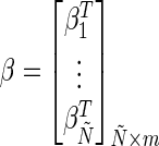and .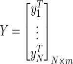

ELM has several interesting and significant features that are different from the traditional popular gradient-based learning algorithms (e.g., feedforward neural networks^20,23). The learning speed of ELM is extremely fast, and it has good generalization performance. More important is that the ELM learning algorithm is much simpler than most learning algorithms for feedforward neural networks.²⁴ Many gradient-based learning algorithms can be used for feedforward neural networks with more than one hidden layer, whereas the ELM algorithm at its present form is still only valid for SLFNs. Fortunately, it has been proved that SLFNs can approximate any continuous function and implement any classification application.²⁴ Thus, reasonably speaking, the ELM algorithm can be efficiently used in many applications, including BG prediction.

SVR model forecasting

SVR is an attractive approach for modeling. Based on the unique theory of the structural risk minimization principle, SVR estimates a function by minimizing an upper bound of the generalization error.²⁵

Supposing that there are training data , where x_i parameters are input patterns and y_i parameters are the associated output values, the basic idea of SVR is to map the data x into a higher-dimensional feature space via a nonlinear mapping and perform a linear regression in this feature space:

(10)

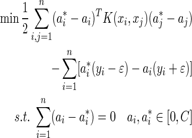
where φ(x) is the feature and w and b are coefficients of SVR. The optimal coefficients can be determined by solving the following minimization problem²⁶:

(11)

where is the kernel function and C is the regularization parameter. There are some kernel functions such as linear kernel, polynomial kernel, and gauss kernel. They are inner products in a very high dimensional space (or infinite dimensional space) but can be computed efficiently by the kernel trick even without knowing φ(x).

According to Karush-Kuhn-Tucker theory,²⁶ the coefficients can be obtained, and the regression function can be define as:

(12)

SVR has been widely applied to time series forecasting.²⁷ However, there still exists an open problem in the practical application of SVR (i.e., selecting parameters to achieve the best prediction performance).

The combined predictor

The BG prediction values from AR, ELM, and SVR methods are denoted as , and , respectively. Next, the final BG prediction by using the proposed adaptive-weighted-average framework is shown in Eq. 13:

(13)

Some tests of the proposed method have been performed in the following section.

Experimental Results and Discussions

To study whether a real-time CGMS can improve glycemic control and the quality of life in patients with T1DM, the JDRF CGM Study Group conducted a randomized clinical trial that included approximately 450 subjects with T1DM.²⁸ Ten subjects were selected randomly from the cohort. By using the CGMS readings of these 10 subjects, the new algorithm and three individual algorithms were compared systematically.

Sparacino et al.⁸ proposed a first-order AR prediction model with time-varying parameters determined using weighted least squares. Gani et al.^5,9 clinically evaluated subject-specific AR models with 30 model orders to improve BG management. The results of Zhao et al.²⁹ show that the best order of the AR model is 7. The experiment results obtained in this study indicate that the best order of the AR model is 5, so the AR model order is fixed at 5 in this study.

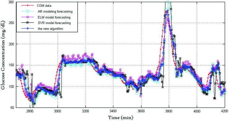
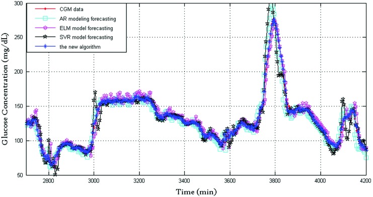
Every time series has 860 points with 5-min sampling period (in total, 4,300 min). These first 500 points (2,500 min) for each subject were used for training ELM, and the other 360 points (1,800 min) are validation data. The BG prediction results between 2,700 and 4,200 min are shown in Figures 1–6. For ELM, the input node number was 3, and the hidden layer node number was 25.

FIG. 1.

Blood glucose prediction results of subject 7 produced by the four algorithms (prediction horizon=30 min). AR, autoregressive; CGM, continuous glucose monitoring; ELM, extreme learning machine; SVR, support vector regression. Color images available online at www.liebertonline.com/dia

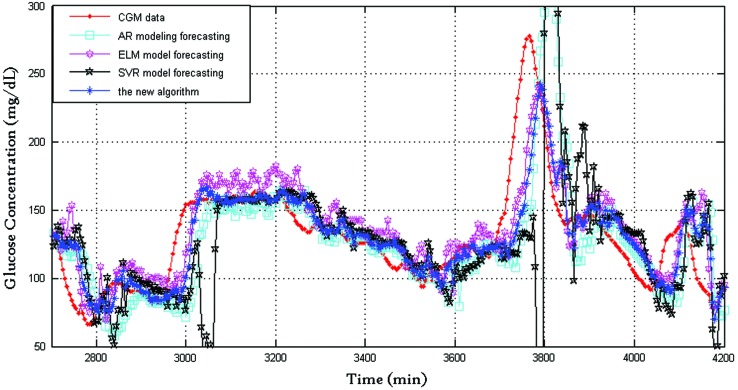
FIG. 6.

Prediction performance of the four algorithms (prediction horizon=45 min). AR, autoregressive; CGM, continuous glucose monitoring; ELM, extreme learning machine; SVR, support vector regression. Color images available online at www.liebertonline.com/dia

Other parameters of SVR were set as C=50 and ɛ=0.5. In addition, local optimization was performed to improve the prediction performance. According to the prediction performance at time k, one kernel function was selected from the different kernel functions linear kernel, polynomial kernel, and gauss kernel.

Except for weights, all other parameters of the proposed method were to the same with those of the individual algorithms.

To quantify the prediction performance, the following indices were used:

• 1. Root-mean-square error (RMSE) was used to evaluate the prediction performance. The definition of RMSE is given in the following equation¹¹:

  
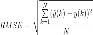
• 2. The relative error analysis is defined as follows:

  

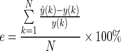
  where and are the predicted and measured values at time k, respectively.

• Clarke error-grid analysis (CEGA)^30–32 is a popular method to evaluate the BG prediction performance. In brief, a larger percentage in Zone A means better prediction performance.

• The “clinical usefulness” of the predicted profile was quantified using the J index.³³ The J index was proposed to optimally design a prediction algorithm by considering two key factors—the regularity of the predicted profile and the time gained due to prediction. The J index can be reliably used as a criterion for comparing different prediction methods.

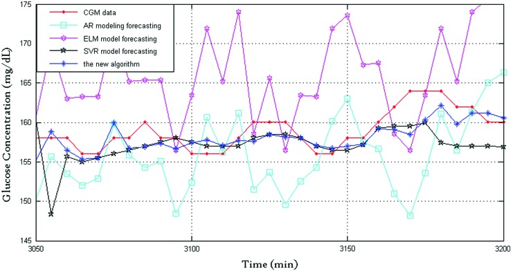
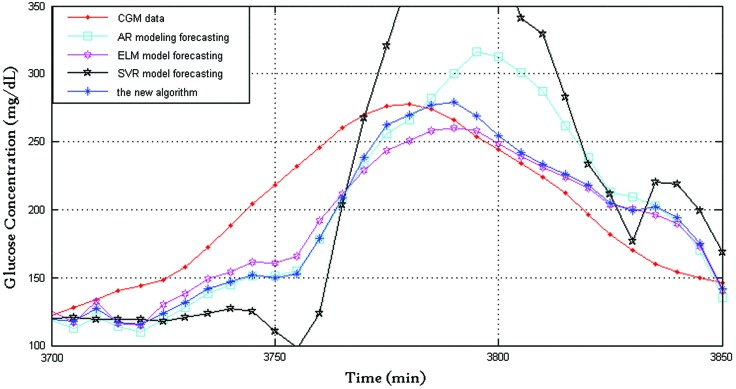
Figure 1 shows the prediction performance of the four algorithms with 30-min prediction horizon, where the dotted line indicates CGMS readings and the star line indicates BG values predicted by the proposed algorithm. For clarity, Figure 2 shows the prediction performance between 3,050 and 3,200 min: the CGMS data in this time are steady, and the SVR provides a good prediction performance of the three algorithms. The new framework tends to trust the SVR forecasting. The new framework provided the best prediction performance because of the time-varying weights. Figure 3 shows the prediction performance between 3,700 and 3,850 min. The rate of change in this time is violent. At approximately 3,800 min, both AR and SVR show large prediction errors in the same direction. The ELM also has an error but in the opposite direction. At this time point, the proposed framework has a satisfactory performance, and the delay of the new algorithm is close to those of AR and SVR. The RMSE values of the AR, ELM, and SVR algorithms and the new framework are 26.1, 20.5±1.7, 50.9, and 19.0±0.3, respectively, and the corresponding relative error values are 9.5, 9.8±0.4, 17.1, and 7.3±0.1, respectively. It is clear that the new framework has the best prediction performance.

FIG. 2.

Prediction performance of the four algorithms between 3,050 and 3,200 min. AR, autoregressive; CGM, continuous glucose monitoring; ELM, extreme learning machine; SVR, support vector regression. Color images available online at www.liebertonline.com/dia

FIG. 3.

Prediction performance of the four algorithms between 3,700 and 3,850 min. AR, autoregressive; CGM, continuous glucose monitoring; ELM, extreme learning machine; SVR, support vector regression. Color images available online at www.liebertonline.com/dia

A comparison of the prediction performance between the proposed framework and the three individual algorithms shows that the prediction performance of the adaptive-weighted-average framework is far superior to that of the three algorithms in most situations studied herein. The framework makes the best use of the advantages and bypasses the disadvantages by adjusting the time-varying weight. As shown in Figure 1, the AR model forecasting has a strong tracking ability, and the delay between the prediction and the true value is acceptable. The ELM model forecasting has a good accuracy, and its prediction is steady and smooth. When the data were smooth, SVR model forecasting had a good prediction performance. The framework inherits the advantage of AR, ELM, and SVR. It has a better accuracy but a smaller delay. At the same time, the framework bypasses the disadvantages. For example, when the rate of change of BG is large, the accuracy of SVM is poor.

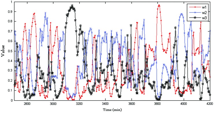
Figure 4 shows the weights of the adaptive-weighted-average framework. It can be seen that the weight is time varying (i.e., when dealing with different data, the framework tends to trust different algorithms). For example, from 3,050 to 3,200 min, the weight w₃ is far ahead of the others; this means the SVR plays an important role in this period.

FIG. 4.

Time-varying weights in the combined framework (prediction horizon=30 min). The “•” line represents the weight of autoregression, the “×” line represents the weight of extreme learning machine, and the “★” line represents the weight of support vector regression. Color images available online at www.liebertonline.com/dia

Figures 5 and 6 show the BG prediction results of the four algorithms with prediction horizons of 15 and 45 min, respectively. The comparing relationships of these algorithms in these two cases (prediction horizon=15 and 45 min) are similar to those of the case when prediction horizon=30 min.

FIG. 5.

Prediction performance of the four algorithms (prediction horizon=15 min). AR, autoregressive; CGM, continuous glucose monitoring; ELM, extreme learning machine; SVR, support vector regression. Color images available online at www.liebertonline.com/dia

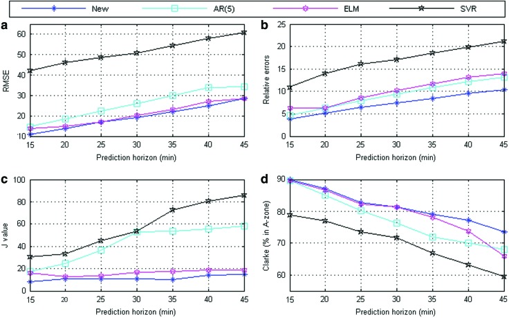
Figure 7 shows the prediction performance of different prediction horizons. It is clear that the proposed framework is better than the other three algorithms in terms of RMSE (mg/dL), relative error, J value, and CEGA (% in Zone A).

FIG. 7.

Prediction performance of the four algorithms (between the different prediction horizons): (a) root-mean-square error (RMSE) values under different prediction horizons; (b) relative errors under different prediction horizons; (c) J values under different prediction horizons; and (d) percentage values in Clarke error-grid analysis Zone A under different prediction horizons. Color images available online at www.liebertonline.com/dia

Tables 1–4 summarize BG prediction accuracy for the 10 subjects in terms of RMSE (mg/dL), relative error, J value, and CEGA (% in Zone A). Because of the randomness of ELM, 50 groups of Monte Carlo simulations were run for both the ELM and the new algorithm.

Table 1.

Root-Mean-Square Error Values for 10 Subjects

	Subject
	1	2	3	4	5	6	7	8	9	10
AR	29.5	11.3	42.6	25.4	18.5	25.4	26.1	14.9	13.6	16.5
SVR	43.5	14.2	61.7	38.2	26.3	38.2	50.9	28.5	18.6	16.9
ELM	33.4±1.2	18.8±4.9	33.9±0.8	20.4±1.9	20.7±2.1	20.5±1.7	20.5±1.7	11.8±0.3	13.0±0.7	14.4±0.4
New	22.8±0.2	9.7±0.2	23.5±0.8	18.6±0.3	15.6±0.2	18.7±0.4	19.0±0.3	11.4±0.4	11.8±0.4	12.7±0.1

Fifty groups of Monte Carlo simulations were run for both extreme learning machine (ELM) and the new algorithm. Data are mean±SD values.

AR, autoregressive; SVR, support vector regression.

Table 4.

Clarke Error-Grid Analysis (Percentage in Zone A) for Glucose from 10 Subjects (%)

	Subject
	1	2	3	4	5	6	7	8	9	10
AR	67.1	88.6	44.3	75.6	81.6	75.6	76.2	80.2	81.9	80.5
SVR	66.6	86.9	45.8	67.4	76.2	67.4	71.7	75.0	73.1	78.2
ELM	68.8±0.9	79.7±2.5	47.6±1.0	77.0±0.6	79.1±1.8	77.1±0.2	81.2±0.4	85.9±0.2	81.0±1.0	79.8±0.8
New	79.6±0.4	90.2±0.4	62.6±1.1	79.0±0.6	85.7±0.3	79.0±0.5	80.6±0.2	85.8±0.8	84.1±0.8	82.1±1.1

Fifty groups of Monte Carlo simulations were run for both extreme learning machine (ELM) and the new algorithm. Data are mean±SD values.

AR, autoregressive; SVR, support vector regression.

Tables 1–4 indicate that the prediction performances of the AR model forecasting and ELM forecasting are similar. For example, for the average RMSE in Table 1, the AR model forecasting and ELM forecasting show good performance in different subjects, and the prediction performance of the SVR forecasting is poor. The adaptive-weighted-average framework is far ahead of the other three algorithms with respect to the four indices. Tables 1, 2, and 4 show that the prediction performance is better and the predictive accuracy is higher while the indices are smaller. For almost all cases, the three indices provided by new algorithm are smaller than the other algorithms. In Table 3, the J value of the new framework is far less than that of the others. According to a previous study,³³ the lower the J value, the better the prediction performance, and the smaller the delay between the prediction and measures. In all, there are 4×10=40 different cases in Tables 1–4, and the proposed framework showed the best prediction performances in 37 cases (i.e., it produced the best prediction performance in 92.5% of situations).

Table 2.

Relative Errors for 10 Subjects

	Subject
	1	2	3	4	5	6	7	8	9	10
AR	13.2	6.8	28.7	9.9	7.7	9.9	9.4	10.0	10.1	6.7
SVR	15.7	8.1	30.2	14.3	9.6	14.3	17.1	15.1	13.8	6.8
ELM	14.5±0.5	13.5±3.0	23.9±0.6	9.1±0.2	8.1±0.4	9.1±0.2	9.8±0.4	8.6±0.4	10.0±0.3	6.2±0.4
New	8.6±0.1	5.9±0.1	16.6±0.7	8.0±0.1	6.2±0.1	7.8±0.1	7.3±0.1	7.5±0.3	8.7±0.3	5.1±0.1

Fifty groups of Monte Carlo simulations were run for both extreme learning machine (ELM) and the new algorithm. Data are mean±SD values.

AR, autoregressive; SVR, support vector regression.

Table 3.

J Values for 10 Subjects

	Subject
	1	2	3	4	5	6	7	8	9	10
AR	37.1	33.1	64.8	68.0	67.8	68.0	52.8	51.6	60.9	44.7
SVR	84.3	43.8	101.4	137.7	73.5	137.7	53. 3	236.1	146.3	33.9
ELM	36.3±11.0	59.9±21.1	27.3±2.0	34.4±18.3	69.3±21.9	33.2±13.1	16.8±6.6	43.6±6.6	54.6±7.7	19.1±1.7
New	15.9±0.3	32.7±1.2	24.2±2.3	25.7±3.2	25.1±1.5	27.2±3.5	12.0±2.1	37.5±3.3	51.5±4.5	23.4±0.8

Fifty groups of Monte Carlo simulations were run for both extreme learning machine (ELM) and the new algorithm. Data are mean±SD values.

AR, autoregressive; SVR, support vector regression.

Thus, the adaptive-weighted-average framework has the best BG prediction performance among the four algorithms in different cases because the framework absorbs the advantages of the three individual algorithms and bypasses their disadvantages. In contrast, the proposed framework has great robustness not only with respect to data variations but also with respect to prediction horizon variations.

Conclusions

The adaptive-weighted-average framework proposed in this study has several significant advantages. First, it has a wide range of applications (i.e., it has great robustness with respect to variations on data characteristic, patients, and prediction horizons). Second, according to the experimental results, the adaptive-weighted-average framework achieves the best prediction performance compared with the individual algorithms. More important is that the adaptive-weighted-average framework is universal (i.e., it can combine any prediction algorithm). It is hoped that this framework could be used in clinical practice to integrate other prediction algorithms.

Acknowledgments

This work was supported by the National Natural Science Foundation of China (grant 61074081), the Doctoral Fund of the Ministry of Education of China (grant 20100010120011), the Beijing Nova Program (grant 2011025), and the Fok Ying-Tong Education Foundation (grant 131060).

Author Disclosure Statement

No competing financial interests exist.

References

- 1.Bode B. Gross K. Rikalo N. Schwartz S. Wahl T. Page C. Gross T. Mastrototaro J. Alarms based on real-time sensor glucose values alert patients to hypo- and hyperglycemia: the Guardian continuous monitoring system. Diabetes Technol Ther. 2004;6:105–113. doi: 10.1089/152091504773731285. [DOI] [PubMed] [Google Scholar]
- 2.Lu Y. Gribok AV. Ward WK. Reifman J. The importance of different frequency bands in predicting subcutaneous glucose concentration in type 1 diabetic patients. IEEE Trans Biomed Eng. 2010;57:1837–1844. doi: 10.1109/TBME.2010.2047504. [DOI] [PubMed] [Google Scholar]
- 3.CareLink personal software [EO/OL] www.professional.medtronicdiabetes.com/carelink-personal-software. [May 7;2013 ]. www.professional.medtronicdiabetes.com/carelink-personal-software
- 4.Cobelli C. Dalla Man C. Sparacino G. Magni L. Nicolao GD. Kovatchev BP. Diabetes: models, signals, and control. IEEE Rev Biomed Eng. 2009;2:54–96. doi: 10.1109/RBME.2009.2036073. [DOI] [PMC free article] [PubMed] [Google Scholar]
- 5.Gani A. Gribok AV. Rajaraman S. Ward WK. Reifman J. Predicting subcutaneous glucose concentration in humans: data-driven glucose modeling. IEEE Trans Biomed Eng. 2009;56:246–255. doi: 10.1109/TBME.2008.2005937. [DOI] [PubMed] [Google Scholar]
- 6.Lu Y. Rajaraman S. Ward WK. Vigersky RA. Reifman J. Predicting human subcutaneous glucose concentration in real time: a universal data-driven approach. 33rd Ann Int Conf Proc IEEE Eng Med Biol Soc. 2011;2011:4945–4949. doi: 10.1109/IEMBS.2011.6091959. [DOI] [PubMed] [Google Scholar]
- 7.Palerm CC. Wilis JP. Desemone J. Bequette BW. Hypoglycemia prediction and detection using optimal estimation. Diabetes Technol Ther. 2005;7:3–15. doi: 10.1089/dia.2005.7.3. [DOI] [PubMed] [Google Scholar]
- 8.Sparacino G. Zanderigo F. Corazza S. Maran A. Facchinetti A. Cobelli C. Glucose concentration can be predicted ahead in time from continuous glucose monitoring sensor time-series. IEEE Trans Biomed Eng. 2007;54:931–937. doi: 10.1109/TBME.2006.889774. [DOI] [PubMed] [Google Scholar]
- 9.Gani A. Gribok AV. Lu Y. Ward WK. Viersky RA. Reifman J. Universal glucose models for predicting subcutaneous glucose concentration in humans. IEEE Trans Inf Technol Biomed. 2010;14:157–165. doi: 10.1109/TITB.2009.2034141. [DOI] [PubMed] [Google Scholar]
- 10.Ståhl F. Johansson R. Short-term diabetes blood glucose prediction based on blood glucose measurements. Conf Proc IEEE Eng Med Biol Soc. 2008;2008:291–294. doi: 10.1109/IEMBS.2008.4649147. [DOI] [PubMed] [Google Scholar]
- 11.Chee F. Fernando TL. Savkin AV. van Heeden V. Expert PID control system for blood glucose control in critically ill patients. IEEE Trans Inf Technol Biomed. 2003;7:419–426. doi: 10.1109/titb.2003.821326. [DOI] [PubMed] [Google Scholar]
- 12.Allam F. Nossair Z. Gomma H. Ibrahim I. Abd-El Salam M. Prediction of subcutaneous glucose concentration for type-l diabetic patients using a feed forward neural network. Int Conf Comput Eng Systems (ICCES) 2011;2011:129–134. [Google Scholar]
- 13.Fan S. Chen L. Short-term load forecasting based on an adaptive hybrid method. IEEE Trans Power Systems. 2006;21:392–401. [Google Scholar]
- 14.Yamakoshi Y. Ogawa M. Yamakoshi T. Satoh M. Nogawa M. Tanaka S. Tamura T. Rolfe P. Yamakoshi K. A new non-invasive method for measuring blood glucose using instantaneous differential near infrared spectrophotometry. Conf Proc IEEE Eng Med Biol Sci. 2007;2007:2964–2967. doi: 10.1109/IEMBS.2007.4352951. [DOI] [PubMed] [Google Scholar]
- 15.Tanaka S. Motoi K. Nogawa M. Yamakoshi T. Yamakoshi KI. Feasibility study of a urine glucose level monitor for home healthcare using near infrared spectroscopy. Conf Proc IEEE Eng Med Biol Soc. 2008;2008:6001–6003. doi: 10.1109/IEMBS.2006.260515. [DOI] [PubMed] [Google Scholar]
- 16.Sandham WA. Lehmann ED. Hamilton DJ. Sandilands ML. Simulating and predicting blood glucose levels for improved diabetes healthcare. Conf Proc Adv Med Signal Inf Process. 2008;2008:1–4. [Google Scholar]
- 17.Dassau E. Jovanovič L. Cameron F. Chase HP. Lee H. Wilson DM. Bequette BW. Buckingham BA. Zisser H. Doyle FJ., III Real-time hypoglycemia prediction suite using continuous glucose monitoring. Diabetes Care. 2010;33:1249–1254. doi: 10.2337/dc09-1487. [DOI] [PMC free article] [PubMed] [Google Scholar]
- 18.Buckingham B. Caswell K. Chase HP. Wilkinson J. Dassau E. Cameron F. Cobry E. Lee H. Clinton P. Bequette BW. Gage V. Doyle FJ., III Prevention of nocturnal hypoglycemia using predictive alarm algorirhms and insulin pump suspension. Diabetes Care. 2010;33:1013–1017. doi: 10.2337/dc09-2303. [DOI] [PMC free article] [PubMed] [Google Scholar]
- 19.Wang T. Zhang T. Forecast Combination: Theory Method and Application [in Chinese] Beijing: Social Sciences Academic Press; 2008. [Google Scholar]
- 20.Huang G-B. Zhu Q-Y. Siew C-K. Extreme learning machine: theory and applications. Neurocomputing. 2006;70:489–501. [Google Scholar]
- 21.Huynh HT. Won T. Hematocrit estimation from transduced current patterns using single hidden layer feedforward neural networks. Conf Proc Convergence Inf Technol. 2007;2007:1384–1388. [Google Scholar]
- 22.Liang N-Y. Huang G-B. Saratchandran P. Sundararajan N. A fast and accurate online sequential learning algorithm for feedforward networks. IEEE Trans Neural Netw. 2006;17:1411–1423. doi: 10.1109/TNN.2006.880583. [DOI] [PubMed] [Google Scholar]
- 23.Deng W. Zheng Q. Chen L. Regularized extreme learning machine. IEEE Symp Comput Intelligence Data Mining. 2009;2009:389–395. [Google Scholar]
- 24.Huang G-B. Zhou H. Ding X. Zhang R. Extreme learning machine for regression and multiclass classification. IEEE Trans Systems Man Cybernet Part B Cybernet. 2012;42:513–529. doi: 10.1109/TSMCB.2011.2168604. [DOI] [PubMed] [Google Scholar]
- 25.Nuryani N. Ling SSH. Nguyen H. Electrocardiographic signals and swarm-based support vector machine for hypoglycemia detection. Ann Biomed Eng. 2012;40:934–945. doi: 10.1007/s10439-011-0446-7. [DOI] [PubMed] [Google Scholar]
- 26.Smola AJ. Scholkopf B. A tutorial on support vector regression. Stat Comput. 2004;14:199–222. [Google Scholar]
- 27.Wang W. Time series prediction based on SVM and GA. Conf Proc Electron Measure Instrum. 2007;2007:2-307–2-310. [Google Scholar]
- 28.JDRF CGM Study Group. JDRF randomized clinical trial to assess the efficacy of real-time continuous glucose monitoring in the management of type 1 diabetes: research design and methods. Diabetes Technol Ther. 2008;10:310–321. doi: 10.1089/dia.2007.0302. [DOI] [PubMed] [Google Scholar]
- 29.Zhao C. Dassau E. Jovanovič L. Zisser HC. Doyle III FJ. Seborg DE. Predicting subcutaneous glucose concentration using a latent-variable-based statistical methods for type 1 diabetes mellitus. J Diabetes Sci Technol. 2012;6:617–633. doi: 10.1177/193229681200600317. [DOI] [PMC free article] [PubMed] [Google Scholar]
- 30.Sivanathan S. Naumova V. Dalla Man C. Facchinetti A. Renard E. Cobelli C. Pereverzyev SV. Assessment of blood glucose predictors: the prediction-error grid analysis. Diabetes Technol Ther. 2011;13:1–10. doi: 10.1089/dia.2011.0033. [DOI] [PubMed] [Google Scholar]
- 31.Kovatchev BP. Evaluating the accuracy of continuous glucose-monitoring sensors: continuous glucose-error grid analysis illustrated by TheraSense Freestyle Navigator data. Diabetes Care. 2004;27:1922–1928. doi: 10.2337/diacare.27.8.1922. [DOI] [PubMed] [Google Scholar]
- 32.Kovatchev BP. King C. Breton M. Anderson S. Clarke W. Clinical assessment and mathematical modeling of the accuracy of continuous glucose sensors (CGS) Conf Proc IEEE Eng Med Biol Soc. 2006;2006:71–74. doi: 10.1109/IEMBS.2006.260114. [DOI] [PubMed] [Google Scholar]
- 33.Facchinetti A. Sparacino G. Trifoglio E. Cobelli C. A new index to optimally design and compare CGM glucose prediction algorithms. Diabetes Technol Ther. 2011;13:111–119. doi: 10.1089/dia.2010.0151. [DOI] [PubMed] [Google Scholar]