Solid-phase chromosome conformation capture for structural characterization of genome architectures

Abstract

We developed Tethered Conformation Capture (TCC), a method for genome-wide mapping of chromatin interactions. By implementing solid-phase ligation, TCC substantially enhanced the signal-to-noise ratio and thus, enabled a detailed analysis of inter-chromosomal interactions. We identified a group of regions in each chromosome that predominantly mediate inter-chromosomal interactions. These regions are marked by high transcriptional activity, suggesting that their interactions are mediated by transcription factories. Each of these regions interacts with numerous other such regions throughout the genome in an indiscriminate fashion, partly driven by the accessibility of the partners. Therefore, it is likely that a different combination of interactions is present in different cells. Accommodating this variability, we developed a computational method to translate the TCC data into physical chromatin contacts in a population of three-dimensional genome structures. Statistical analysis of the resulting population demonstrates that the indiscriminate properties of inter-chromosomal interactions is consistent with the well-known architectural features of the human genome.

INTRODUCTION

The three-dimensional (3D) organization of the eukaryotic genome plays important roles in nuclear functions^{1, 2}. However, few structural details of chromatin organization have been delineated at the genomic scale. For instance, individual chromosomes are localized in spatially distinct volumes known as the chromosome territories³, which tend to occupy preferential positions with respect to the nuclear periphery^{4, 5}. Moreover, the territories of different chromosomes form extensive interactions⁶, and high-density gene clusters can extend outside of the bulk of their chromosome’s territory⁷. Nevertheless, the internal organization of chromosome territories and the mechanisms that govern the interactions between them are not well-understood.

Chromosome conformation capture (3C)-based techniques have emerged as powerful tools for mapping chromatin interactions^8-16. The genome-wide application of these techniques has revealed that functional activity can determine the association preferences of loci within each chromosome¹⁰. Further understanding of the spatial organization of chromosomes, however, is limited by several factors. For one, low signal-to-noise ratios in conformation capture experiments compromise their ability to map low frequency interactions, especially those between chromosome territories. Additionally, the data represent an ensemble average of genome structures in the cell population, wherein individual structures may significantly differ from each other^17-19. Coupled with the enormous size of the genome, this heterogeneity of genome architecture makes translating conformation capture data into 3D structural models challenging. As a result, even as genome-wide conformation capture data have been used to propose theoretical folding models¹⁰, they have not yet been employed for determining the corresponding 3D structures of the entire genome in mammalian cells.

For the genome-wide mapping of chromatin contacts, we have developed the Tethered Conformation Capture (TCC) technology, a modified conformation capture method in which key reactions are carried out on solid-phase instead of in solution. This tethering strategy leads to higher signal-to-noise ratios, enabling an in-depth analysis of inter-chromosomal interactions. We show that a specific group of functionally active loci are more likely to form inter-chromosomal contacts and that most of these contacts are a result of indiscriminate encounters between loci that are accessible to each other. We also introduce a structural modeling procedure that calculates a population of 3D genome structures from the TCC data. We show that the calculated population reproduces the hallmarks of chromosome territory positioning in agreement with independent fluorescence in situ hybridization (FISH) studies. This population-based approach allows for a probabilistic analysis of the spatial features of the genome, a capability that can accommodate the wide range of cell-to-cell structural variations that are observed in mammalian genomes^{17, 20}.

RESULTS

Detecting genome-wide chromatin contacts using TCC

To identify chromatin interactions using TCC (Fig. 1), native chromatin contacts were preserved by chemically crosslinking DNA and proteins. The DNA was then digested with a restriction enzyme, and, after cysteine biotinylation of proteins, the protein-bound fragments were immobilized at a low surface density on streptavidin-coated beads. The immobilized DNA fragments were then ligated while tethered to the surface of the beads. Finally, ligation junctions were purified, and ligation events were detected by massively parallel sequencing, a process which revealed the genomic locations of the pairs of loci that had formed the initial contacts (Fig. 1).

Figure 1. Overview of Tethered Conformation Capture (TCC).

Cells are treated with formaldehyde, which covalently crosslinks proteins (purple ellipses) to each other and to DNA (orange and blue strings). (1) The chromatin is solubilized and its proteins are biotinylated (purple ball and stick). DNA is digested with a restriction enzyme that generates 5’ overhangs. (2) Crosslinked complexes are immobilized at a very low density on the surface of streptavidin coated magnetic beads (grey arc) through the biotinylated proteins; non-crosslinked DNA fragments are removed. (3) The 5’ overhangs are filled in with an α-thio-triphosphate containing nucleotide analog (the yellow nucleotide in the inset), which is resistant to exonuclease digestion, and a biotinylated nucleotide analog (the red nucleotide with the purple ball and stick in the inset) to generate blunt ends. (4) Blunt DNA ends are ligated. (5) Crosslinking is reversed and DNA is purified. The biotinylated nucleotide is removed from non-ligated DNA ends using E. coli exonuclease III while the phosphorothioate bond protects DNA fragments from complete degradation. (6) The DNA is sheared and fragments that include a ligation junction are isolated on streptavidin-coated magnetic beads, but this time through the biotinylated nucleotides. (7) Sequencing adaptors are added to all DNA molecules to generate a library. (8) Ligation events are identified using paired-end sequencing. The steps that are unique to the TCC strategy are biotinylation of the chromatin proteins, immobilization of crosslinked complexes on the beads, performing ligation and other reactions on the beads, and the use of exonuclease-resistance nucleotide analogs for the purification of ligated DNA fragments from the non-ligated.

We applied TCC, using HindIII as the restriction enzyme, to map the chromatin contacts in GM12878 human lymphoblastoid cells (Supplementary Table 1). As an example of non-tethered conformation capture, we also applied Hi-C¹⁰ to the same cell line using identical cell counts and crosslinking conditions. The resulting contact frequency maps (Fig. 2a,b and Supplementary Fig. 1a) showed that TCC accurately reproduces the patterns observed in Hi-C results (Pearson’s r for genome-wide comparison = 0.96, p-value < 10^-16). Additionally, the general features of genome-wide conformation capture data that were described previously¹⁰ were also observed in our data (Fig. 2a,b and Supplementary Fig. 1a,b,c).

Figure 2. Tethering improves the signal-to-noise ratio of conformation capture.

(a,b) TCC can reproduce the results obtained by Hi-C¹⁰. A genome-wide contact frequency map is compiled from the ligation frequency data generated by tethered (TCC) (a) and non-tethered (Hi-C) (b) conformation capture. The portion of each map that corresponds to the intra-chromosomal contacts of chromosome 2 is shown. The intensity of the red color in each position of the map represents the observed frequency of contact between corresponding segments of the chromosome which are shown on the top and to the left of the map. In these maps, chromosomes 2 is divided into segments that span 277 HindIII sites each, resulting in 258 segments of ∼1 Mb (Supplementary Methods). A pair of tick marks on the ideogram encompasses 4986 HindIII sites. In this and other figures, the white lines in the heatmaps mark the unalignable region of the centromeres. See Supplementary Figure 1a for the tethered contact frequency maps of all the other chromosomes.

(c) The observed fractions of intra (dark red) and inter-chromosomal (light blue) ligations in tethered (T) and non-tethered (NT) libraries produced using HindIII or MboI. The random ligation (RL) bar represents the expected fractions if all ligations occurred between non-crosslinked DNA fragments. For the non-tethered MboI library only, these fractions were determined by sequencing 160 individual DNA molecules from three replicates of the experiment. See Supplementary Table 1 for the sequencing output information of the other three libraries.

(d,e) The genome-wide enrichment map for chromosome 2, compiled from the tethered (d) and non-tethered (e) HindIII libraries. Enrichment is calculated as the ratio of the observed frequency in each position to its expected value; expected values were obtained assuming completely random ligations (Methods). Red and light blue respectively indicate enrichment and depletion of a contact in accordance with the color key between the panels. Chromosome 2 (left) extends along the Y-axis while all 23 chromosomes (top) extend along the X-axis. The zoomed panel to the right of each map magnifies the section that corresponds to contacts between the small arm of chromosome 2 and chromosomes 20, 21, 22, and X. For these maps, each chromosome is divided into segments that span 558 HindIII sites, leading to respectively 116 and 1384 segments of ∼1.5 Mb for chromosome 2 and all other chromosomes. A pair of tick marks on chromosome 2 spans 5022 HindIII sites.

Improved signal-to-noise ratio in tethered libraries

One of the main sources of noise in conformation capture experiments is random intermolecular ligations between DNA fragments that are not crosslinked to each other^{9, 21}. Because randomly selected DNA fragments are more likely to originate from different chromosomes, these ligations tend to be exceedingly inter-chromosomal. We, therefore, measured the fraction of inter-chromosomal ligations in our tethered (TCC) and non-tethered (Hi-C) HindIII libraries to compare their relative noise levels (Fig. 2c). In the tethered library, this fraction is almost half that of the non-tethered library. We also compared the average difference between the observed inter-chromosomal contact frequencies in each library and those expected from completely random inter-molecular ligations. This difference is twice as large in the tethered library compared to the non-tethered library (Supplementary Methods). Together, these observations indicate that the noise from random inter-molecular ligations is considerably lower in the tethered library.

We also generated tethered and non-tethered libraries using the 4-cutter MboI instead of HindIII. MboI results in a shorter size and a higher concentration of DNA fragments, thereby increasing the probability of random inter-molecular ligations. Consequently, the fraction of inter-chromosomal ligations increased substantially in the non-tethered MboI library (Fig. 2c). By contrast, it showed only a modest increase in the tethered MboI library. This result demonstrates that tethered libraries are minimally affected by the concentration of DNA fragments, confirming that most ligations in these libraries are between DNA fragments that are crosslinked to each other.

An improved signal-to-noise ratio allows a more accurate analysis of contacts with relatively low frequencies such as interactions between chromosomes (Supplementary Fig. 1d). For instance, several interactions between the small arm of chromosome 2 and chromosomes 20, 21, and 22 are clearly enriched in the tethered HindIII library (Fig. 2d) but not the non-tethered HindIII library (Fig. 2e).

Two classes of regions with different intra-chromosomal contact behaviors

We first analyzed the contact pattern within each chromosome. We defined the contact profile of a region as the ordered list of frequency values for its contacts with all the other regions in the genome (Methods). The Pearson’s correlation between two intra-chromosomal contact profiles is a similarity measure for the corresponding regions’ contact behaviors. Using this measure and confirming a previous study¹⁰, we observed that each chromosome can be divided into two classes of regions with anti-correlated intra-chromosomal contact profiles (Fig. 3a and Supplementary Fig. 2a). At any given genomic distance, regions in the same class contact each other more frequently than regions in different classes (Supplementary Fig. 2b). One of these classes, here referred to as the “active class”, is significantly enriched for the presence and expression of genes, DNase hypersensitivity, and activating histone modifications¹⁰(Supplementary Fig. 2c). The other class, here referred to as “inactive”, displays the opposite behavior (Supplementary Fig. 2c).

Figure 3. Intra-chromosomal interactions.

(a) Correlation map and class assignment for chromosome 2. The color of each position in the map represents the Pearson’s correlation between the intra-chromosomal contact profiles of the corresponding two segments of the chromosome to the left and on top (the ideogram of the chromosome has only been shown to the left, but the X-axis of the map also represents the chromosome). The color key is shown on the bottom-right corner of the figure. To assign each segment to the active (orange blocks on top of the map) or the inactive (purple blocks on top of the map) class, principal component analysis (PCA) is used to calculate the EIG variable (plotted on top of the assignment blocks) for each segment. Segments with a positive EIG are assigned to the active class, while those with a negative EIG are assigned to the inactive class. Segments with EIG values close to zero have not been assigned to either class (Methods). The size of each chromosome band is based on the number of HindIII sites it contains. For this map, chromosome 2 is divided into 517 segments of ∼0.5 Mb, each spanning 138 HindIII sites. See Supplementary Figure 2a for correlation maps and class assignments of all the other autosomal chromosomes. Data from the tethered HindIII library are used in this panel and other panels of the figure.

(b) The genome-wide average Pearson’s correlation between intra-chromosomal contact profiles of two active segments (orange), two inactive segments (dark purple), and an active and an inactive segment (gray) plotted against their genomic distance. Each chromosome is divided into segments of 138 HindIII sites, resulting in 6,000 segments of ∼0.5 Mb.

(c) Active-active (left) and inactive-inactive (right) correlation maps for chromosome 2. The color intensity of each point in the map represents the Pearson’s correlation between the “active-only” (left) or “inactive-only” (right) contact profiles of the corresponding segments, whose location in the chromosome has been marked by an arrow on the ideogram of chromosome 2 in the middle. The ideogram shows the positions of the active (orange bars on the left) and inactive (purple bars on the right) segments. The different shades of orange and purple are used only to differentiate the adjacent segments. Each correlation map is calculated following the procedure in (a), except only contacts between active segments (left) or inactive segments (right) are considered. Color-coding is identical to (a) and the key is shown on the bottom-right corner of the figure. The order of segments from left to right is the same as the order from top to bottom. Segment sizes are identical to (a). For similar active-active and inactive-inactive maps of the other large chromosomes see Supplementary Figure 3c.

We asked how the similarity between contact profiles changes with increasing genomic distance between the regions on a chromosome. Interestingly, the contact profiles of the active regions remain similar even when relatively long genomic distances separate them (Fig. 3b). For the inactive regions, in contrast, the contact profile similarity decreases more quickly and dissipates at longer distances (Fig. 3b). Therefore, inactive regions are more likely to associate with their neighboring regions while active regions can associate with a more diverse panel of long-range contact partners.

A special case of this behavior was observed in the interactions between inactive regions of large chromosomes (i.e., 1-6,8,10). The average contact profile similarity decreases abruptly for inactive regions separated by the centromere. Consequently, only inactive regions in the same chromosome arm have similar contact profiles (Supplementary Fig. 3a). The frequency of contacts between inactive regions in different chromosome arms is also significantly lower than would be expected from their sequence separation alone (Supplementary Fig. 3b). These characteristics give rise to a distinctive four-block pattern in the “inactive-only” correlation matrices of the larger chromosomes (Fig. 3c and Supplementary Fig. 3c). In contrast, the contact profile similarity of active regions is largely unaffected by the centromere (Fig. 3c and Supplementary Fig. 3a,c). These results suggest that, in larger chromosomes, inactive regions from opposing chromosome arms are largely inaccessible to each other while active regions can still interact.

High propensity for inter-chromosomal interactions in the active class

We next analyzed the contacts between chromosomes. We began by defining the inter-chromosomal contact probability index (ICP) as the sum of a region’s inter-chromosomal contact frequencies divided by the sum of its inter and intra-chromosomal contact frequencies. ICP, therefore, describes the propensity of a region to forming inter-chromosomal contacts.

Interestingly, we observed large differences in the distribution of ICP between the active and inactive classes. In the inactive class, the vast majority of regions have relatively low ICPs with the exception of a few cases (Fig. 4a and Supplementary Fig. 4a,b). Most of these exceptions flank the unalignable regions of the centromeres, and their high ICP is due to interaction with the centromeric regions of other chromosomes (Supplementary Fig. 5a). Additionally, the centromeric regions of the acrocentric chromosomes are more likely to contact each other than the centromeric regions of the metacentric chromosomes (Supplementary Fig. 5b). Furthermore, we found the highest centromere contact frequencies between chromosomes 13 and 21 and between chromosomes 14 and 22 (Supplementary Fig. 5c). All of these observations are in excellent agreement with previous imaging studies in lymphocytic cells^22-24.

Figure 4. Inter-chromosomal interactions.

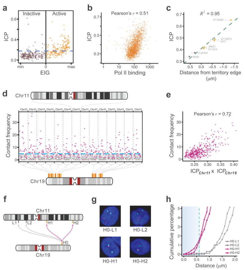
(a) For all segments of chromosome 2, inter-chromosomal contact probability index (ICP) is plotted against EIG. Segments with a positive EIG (orange) belong to the active class, while those with a negative EIG (brown) belong to the inactive class. The blue dashed line separates high-ICP segments: values above the line are significantly larger than the average ICP for inactive segments. Red dots mark those inactive segments with a large ICP that also flank the centromere. For this map, chromosome 2 is divided into 517 segments of ∼0.5 Mb, each spanning 138 HindIII sites. See Supplementary Figure 4a for similar plots of all autosomal chromosomes and Supplementary Figure 4b for the alignment of ICP and EIG values along chromosome 2. See also Supplementary Table 2 for ICP and EIG values of all segments of the genome. In this and other panels of this figure, data from the tethered HindIII library are used.

(b) For all active segments in the genome, ICP is plotted against the binding of RNA polymerase II (pol II). Pol II binding values are reproduced from a ChIP-seq study³⁸ on the GM12878 cells and are in arbitrary units based on alignment frequency (Methods). The p-value of the correlation is smaller than 10^-16. Each point represents a segment of the genome that spans 138 HindIII sites. The X-axis is plotted in a logarithmic scale.

(c) For seven loci on the small arm of chromosome 11, the ICP value is plotted against their average distance from the edge of chromosome 11 territory as measured by FISH²⁷. Positive distance values denote localization within the bulk territory, while negative values denote localization away from the bulk territory. Orange and brown dots represent assignment to the active and inactive classes respectively. Error bars represent ±95% confidence interval²⁷. See Supplementary Figure 4c for more information and a side-by-side comparison of the FISH and TCC data for these loci.

(d) Plotted are the frequencies of all contacts between high-ICP active segments on chromosome 19 and all the segments on chromosome 11. Contacts involving high-ICP active segments on chromosome 11 are shown as purple squares and contacts involving all other segments of this chromosome are shown as grey triangles. Contacts plotted between vertical dotted lines involve the same high-ICP active segment on chromosome 19 and all the segments of chromosome 11. Frequencies above the dashed blue line are significantly higher than the average frequency of contacts between high-ICP active segments on chromosome 19 and inactive segments on chromosome 11 (p-value < 0.04, non-parametric). These frequencies can be considered significantly larger than the noise level, defined as the false-positive contact frequencies due to random inter-molecular ligations. For this plot, each chromosome was divided into ∼1 Mb segments that span 277 HindIII sites resulting in a total of 143 segments for chromosomes 11 and 43 segments for chromosome 19. Among those, 14 segments on chromosome 19 and 28 segments on chromosome 11 were classified as high-ICP active. The locations of the high-ICP active segments in chromosome 19 are marked by an orange bar on the ideogram of the chromosome on the bottom of the panel. The different shades of oranges are used only to differentiate the adjacent segments. See Supplementary Figure 6a for contact profiles of high-ICP active segments in chromosome 19 with all high-ICP active segments in the genome.

(e) For all possible pairs of high-ICP active segments from chromosomes 11 and 19, their contact frequency has been plotted against the product of their ICPs. Same interactions are marked with purple color in (d). The p-value of the correlation is nominal.Other parameters are the same as in (d). See also Supplementary Figure 6b for a similar plot of chromosome 11 with all the other chromosomes and Supplementary Figure 6c for a histogram of the correlations of all 231 possible such plots for autosomal chromosomes.

(f) The layout of 3D-FISH experiments where the localization of a high-ICP active locus on chromosome 19 (H0) relative to four loci on chromosome 11 (H1, H2, L1, and L2) was analyzed in about 1,000 cells per pair of loci. H1 and H2 are high-ICP active, while the L1 and L2 are inactive. The blocks on the chromosomes' ideograms mark the position of each locus (orange for high-ICP active and brown for inactive), and the arrows mark the pair combinations that are analyzed (purple for active-active and grey for active-inactive). See also Supplementary Table 3 for the names and genomic locations of the BAC clones that were used.

(g) An example nucleus from each pair of loci analyzed in 3D-FISH. Nuclei are counterstained with DAPI (blue). In all four nuclei, the hybridization signal of H0 is shown in red and that of the other locus is shown in green.

(h) Cumulative percentage of nuclei that show a pair of hybridization signals closer than a given distance is plotted. Only the closest pair of signals for each nucleus is considered. 1,011, 987, 976, and 998 total nuclei were analyzed in duplicates for H0-L1, H0-L2, H0-H1, and H0-H2 respectively. Distances smaller than 0.6 μm (dashed blue line - arbitrarily selected for visualization purposes) represent colocalizations in a close vicinity where a direct interaction between loci is possible. Because colocalization is required but not sufficient for a direct contact, these values likely provide a ceiling for the fraction of cells that harbor a direct contact between these loci.

In the active class, on the other hand, many regions have high ICPs. In fact, the vast majority of regions with a large ICP belong to the active class (Fig. 4a and Supplementary Fig. 4a,b). For example, in chromosome 2, 90% of the regions with a top 25% ICP are members of the active class (Fig. 4a). Nevertheless, not all the active regions have a large ICP. For instance, about 40% of the active regions in chromosome 2 form relatively few inter-chromosomal contacts, and their ICPs are similar to those of the inactive regions (Fig. 4a). This non-uniform contact behavior may reflect functional variations within this class. Indeed, we observed that those active regions with larger ICPs also show higher RNA polymerase II binding (Fig. 4b) as well as higher total gene expression (Pearson’s r = 0.54, p-value < 10^-15), indicating that higher transcriptional activity is associated with an increased probability of forming inter-chromosomal contacts.

We asked whether the regions’ differences in ICP are reflected in their localization within their chromosomes’ territories. Previous fluorescence imaging studies have shown that highly transcribed regions can frequently extend outside of the bulk territory of their chromosome^{25, 26}. One of these studies analyzed several loci on chromosome 11 in lymphoblastoid cells²⁷. Remarkably, we found that the reported average distances of these loci from the edge of their chromosome territory is strongly correlated with their ICPs (Pearson’s r = 0.98, p-value < 10^-3) (Fig. 4c and Supplementary Fig. 4c). Moreover, the loci that showed preferential localization in the bulk of the chromosome territory in the imaging study are inactive in the TCC data, while those that showed more frequent localization beyond the bulk of the territory are active and have large ICPs(Fig. 4c). While more fluorescence imaging experiments are required to extend this observation to the entire genome, these examples suggest that ICP can also reflect the preferred positions of a locus within the territory of its chromosome.

Indiscriminate interactions between chromosome territories

To further examine the interactions between chromosomes, we analyzed those inter-chromosomal contacts with frequencies clearly above noise level. We refer to these contacts as “significant interactions” (Fig. 4d). Most of these significant interactions are formed by active regions, in particular by those with high ICPs (Fig. 4d). Interestingly, most of these regions interact with numerous other high-ICP active regions throughout the genome (Fig. 4d and Supplementary Fig. 6a). For instance, each of the high-ICP active regions on chromosome 19 forms significant interactions with at least 40% of all the high-ICP active regions on chromosome 11 (Fig. 4d) and many more on other chromosomes (Supplementary Fig. 6a). Moreover, none of these interactions appears to be dominant, and they all have relatively low frequencies (Fig. 4d and Supplementary Fig. 1d). In the case of chromosomes 11 and 19, the significant inter-chromosomal interactions between high-ICP active regions are on average more than seventy times less frequent than intra-chromosomal contacts between neighboring ∼1 Mb regions. The numerosity of these interactions and their low frequencies suggest that each can be present in only a fraction of the cells.

Strikingly, the larger the ICP of the inter-chromosomal contact partners, the higher the observed frequency of their interaction (Supplementary Fig. 6a). Indeed, the contact frequency between a pair of high-ICP active regions shows a positive correlation with the product of their ICPs (Fig. 4e and Supplementary Fig. 6b,c). Based on these observations, it appears that for many high-ICP active regions the probability of forming inter-chromosomal interactions is independent of the identity of their interaction partners. We already established that ICP can be an indicator for the relative position of a region from the edge of the chromosome territory. This correlation, therefore, suggests that the propensity for forming inter-chromosomal contacts between high-ICP active regions is largely governed by the spatial accessibility of the contact partners.

To confirm the existence of inter-chromosomal interactions between high-ICP active regions we measured the colocalization frequency of one probe on chromosome 19 with each of four different probes on chromosome 11 using 3D DNA FISH (Fig. 4f-h and Supplementary Table 3). The chromosome 19 probe was located in a high-ICP active region while the four chromosome 11 probes were equally split between inactive and high-ICP active regions. These measurements showed that, in a small but significant fraction of the cells, the high-ICP active region on chromosome 19 colocalizes with each of its active counterparts on chromosome 11 (Fig. 4h). In contrast, the same region on chromosome 19 is unlikely to localize in proximity to either inactive regions on chromosome 11. These results support the conclusion that high-ICP active regions on different chromosomes can interact and that each interaction occurs in only a small fraction of the cells.

In summary, our observations indicate that most active regions do not exclusively interact with only a few specific regions on other chromosomes, rather they can form interactions indiscriminantly with many high-ICP active regions at different times. These contacts may only be present in the fraction of cells where both interaction partners are mutually accessible.

3D genome structures from conformation capture data

We then asked whether the indiscriminate and numerous low-frequency chromosome interactions can be reconciled with the non-random positioning of chromosome territories with preferred radial positions seen in other studies3-5. Chromatin contacts are observed with a wide range of frequencies, suggesting that many potential contacts are present in only a fraction of cells. In other words, the contacts in TCC data describe not necessarily one structure but represent the average contacts of numerous genome structures in different cells. Therefore, a population of genome structures must be generated in which the resulting variety of structures is statistically consistent with the data. We express this task as an optimization problem with three main components28, 29: (1) a structural representation of chromosomes at an appropriate level of resolution; (2) a scoring function quantifying the structure population’s accordance with the data; and (3) a method for optimizing the scoring function to yield a population of genome structures.

Structural representation: coarse-graining of the chromosomes

The plaid appearance of the contact frequency maps suggests that each chromosome can be partitioned into “blocks” of consecutive regions that share similar contact profiles. To identify these blocks, we applied constrained clustering using the Pearson’s correlation between the regions’ contact profiles as a similarity measure (Fig. 5a, Methods). Optimizing the clustering cutoff divided the haploid genome into 428 “chromatin-block” regions (Supplementary Fig. 7a, Methods). The resulting block-based contact frequency map (Fig. 5b) is highly correlated with the original frequency map (Spearman’s-correlation 0.81, p-value<10-16), confirming that the characteristic longrange contact patterns are preserved (Fig. 5a,b). Several observations indicate that large portions of chromatin regions in any given block are in spatial proximity and predominately occupy the same specific sub-territory in the nucleus. First, the vast majority of contacts are between regions inside a block. Second, across the block borders, the contact probability between neighboring regions is abruptly reduced and an abrupt change in contact profiles is observed. As a first approximation, we defined the sub-territory that is largely occupied by each block region as a globular volume whose spherical radius is approximated by the block size (Fig. 5c and Supplementary Table 4). The structure of a genome is then given by a spatial arrangement of these spheres. Our goal is then to determine a population of genome structures, where in each structure all the 856 spheres of the diploid genome are packed into the nucleus in such a way that their contacts across the population are entirely consistent with the TCC data (Fig. 5d).

Figure 5. Coarse-graining of the contact frequency maps and structural representation of the genome.

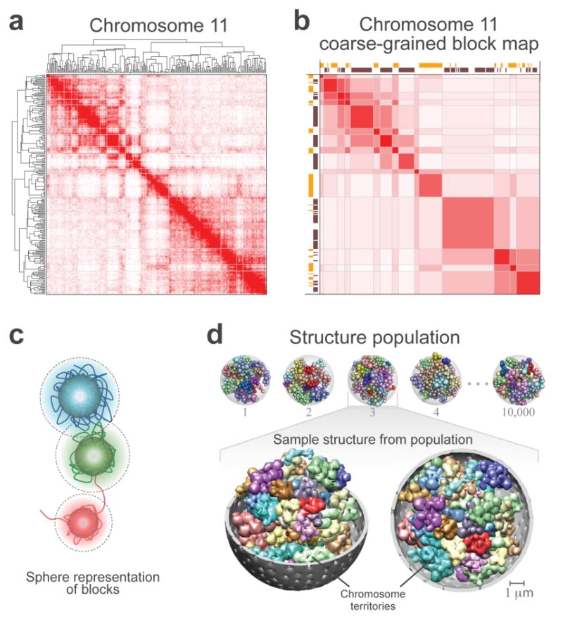
(a) The contact frequency map of chromosome 11 from the tethered HindIII library. The chromosome has been divided into 237 segments each of which covers 166 HindIII sites. Hierarchical constrained clustering was applied using the Pearson’s correlation between the segments’ contact profiles as the similarity measure (Methods). The dendrogram of constrained clustering is shown to the left and on top of the map. The intensity of the red color in each position of the map represents the observed frequency of contact between corresponding segments of the chromosome shown on the top and to the left of the map.

(b) Coarse-grained block matrix of chromosome 11. To identify the blocks, a clustering cutoff was determined following a previously described procedure³⁹. In the block map, the value of an element is the average contact frequency of all the corresponding elements in the contact frequency map. The dimension of the initial contact frequency map is reduced to 15 blocks for chromosome 11 and 428 for the entire genome in the block map. Spearman’s rank correlation coefficient between this block matrix and the contact frequency map in (a) is 0.78. Assignment of segments to the active (orange blocks) and inactive (dark brown blocks) classes are shown to the left and on top of the matrix. The intensity of the red color in each element represents the average of the observed contact frequencies between the corresponding blocks of the chromosome. See Supplementary Figure 7b-d for the coarse-grained genome-wide block matrix.

(c) Sphere representation for chromatin regions in a block. The sphere for each block is defined by two different radii. First, its hard radius (solid sphere) which is estimated from the block sequence length and nuclear occupancy of the genome; the sphere cannot be penetrated within this radius (Methods). Second, its soft radius (dotted line), which is twice that of the hard sphere radius. A contact between two spheres is defined as an overlap between the spheres’ respective soft radii. Also shown is a schematic hypothetical view of the chromatin fiber. For all the block sequence lengths and resulting sphere radii see Supplementary Table 4.

(d) Genome structure population of 10,000. A schematic of the calculated structure population is shown on top. A randomly selected sample from the population is magnified on the buttom. All forty-six chromosome territories are shown. Homologous pairs share the same color. The nuclear envelope is displayed in grey. For visualization purposes, the spheres are blurred in the magnified structure because the use of 2x428 spheres to represent the genome makes the territories appear more discrete than they actually are.

Generating a population of genome structures

We converted the TCC contact frequencies into a set of contact restraints between spheres in all the structures of the population. A restraint can be thought of as generating a “force” between the spheres so that they form a contact. Importantly, any given contact can only be enforced in the fraction of models in the population corresponding to its TCC frequency (Supplementary Methods). If a contact is not enforced, no assumptions are made about the relative positions of the corresponding spheres. Therefore, our method does not correlate contact frequencies with averaged distances; it relies purely on the TCC data by incorporating only the presence or absence of chromatin contacts.

In a diploid cell, most loci are present in two copies. Because the TCC data do not distinguish between these copies, the optimal assignment of each sphere to a specific contact is determined as a part of our optimization process^{28, 30}.

Finally, starting from random positions, we simultaneously optimized the positions of all the spheres in a population of 10,000 genome structures to a score of 0, indicating that no restraint violations remained (Supplementary Methods).

To test how consistent this structure population is with the experiment, the block contact frequency map was calculated from the structure population and compared with the original data. The two are strongly correlated; the average Pearson’s correlation is 0.94, confirming the excellent agreement between contact frequencies in the structure population and experiment (Supplementary Fig. 7b-d). Furthermore, three independently calculated populations showed that our structure population is highly reproducible (Pearson’s r > 0.999), which also indicates that, at this resolution, the size of the model population is sufficiently large (Supplementary Methods).

Structural features of the genome population

Because chromatin contacts in the TCC data are observed over a wide range of frequencies, the resulting population shows a fairly large degree of structural variation (Supplementary Fig. 8a,b). For instance, on average only 21% of contacts are shared between any two structures in the population (Supplementary Fig. 8c). Despite this large heterogeneity, the structure population reveals a distinct and non-random chromosome organization. Specifically, the population clearly identifies the preferred radial positions of chromosomes (Fig. 6a,b and Supplementary Fig. 9b). These positions strongly agree with independent FISH studies in lymphoblasts^{4, 5}: the Pearson’s correlation between the experimental and population-based average positions was 0.71 (p-value < 10^-3) for the 22 chromosomes whose radial positions were previously determined⁴. Instead, radial positions in a control population generated without TCC data did not agree with the experiment (Pearson’s r = -0.2, Supplementary Fig. 9a), indicating that the TCC data are responsible for generating the correct radial distributions seen in the imaging experiments⁴. In general, the radial chromosome positions tend to increase with their size, with some noticeable exceptions (Fig. 6b). One of these cases is the radial positions of chromosomes 18 and 19 which, despite their similar size, we observed at significantly different positions⁵. Chromosome 19 is located closer to the center of the nucleus, while chromosome 18 is preferentially located closer to the nuclear envelope (Fig. 6a). Furthermore, the homologous copies of chromosome 18 are often distant from each other while those of chromosome 19 are often closely associated (Fig. 6a and Supplementary Fig. 9b), in agreement with independent experimental evidence⁵.

Figure 6. Population-based analysis of territory localizations in the nucleus.

(a) The distribution of the radial positions for chromosomes 18 (red dashed line) and 19 (blue solid line), calculated from the genome structure population. Radial positions are calculated for the center of mass of each chromosome and are given as a fraction of the nuclear radius. See Supplementary Figure 9b for the radial distribution of all chromosome territories.

(b) The average radial position of all chromosomes plotted against their size. Error bars mark the standard deviation. For the radial positions from a control genome structure population generated without TCC data see Supplementary Figure 9a.

(c) Clustering of chromosomes with respect to the average distance between the center of mass of each chromosome pair in the genome structure population (shorter to longer average distance is colored by gradual purple to white). The clustering dendogram, which identifies two clusters is shown on top.

(d) (Left panels) The density contour plot of the localization probability for all chromosomes in cluster 1 (top panel) and cluster 2 (bottom panel) calculated from all the structures in the genome structure population. The rainbow color-coding ranges from blue (minimum value) to red (maximum value). (Right panels) Shown is a representative genome structure from the genome structure population. Chromosome territories are shown for all chromosomes in cluster 1 (top) and all chromosomes in clusters 2 (bottom). The localization probabilities are calculated following a previously-described procedure²⁸.

Structure based analysis of territory colocalizations

When chromosome territories are clustered based on their average distances, two main groups can be identified (Fig. 6c). The first group (chromosomes 1,11,14-17,19-22) tend to occupy the central region of the nucleus as is evident from their population-based joint localization probabilities (Fig. 6d). These chromosomes also tend to have relatively higher gene densities³¹. The second group (chromosomes 2-10,12,13,18,X) preferentially occupies the periphery of the nucleus (Fig. 6d).

Finally, we observe differences in the local packing between the spheres composed of mainly active or inactive regions. The average distances between spheres of mainly active regions are statistically larger (Supplementary Fig. 9c), suggesting that inactive regions are more densely packed in the structure population in comparison to the active regions.

DISCUSSION

TCC offers improved sensitivity in identifying chromatin interactions. In particular, libraries generated with the tethering strategy have a lower level of random intermolecular ligation compared to those generated by a non-tethered approach (Fig. 2c). The reduced noise level facilitates the analysis of low-frequency contacts such as inter-chromosomal interactions, which can otherwise be lost in the relatively higher background noise (Fig. 2d,e and Supplementary Fig. 10). Because the inter-molecular ligation noise remains low even at substantially increased DNA concentrations, this method also facilitates higher resolution analyses with enzymes that cut the chromatin more frequently.

Two main factors may contribute to this reduction of random inter-molecular ligations in the tethered libraries. First, DNA fragments can only be immobilized when they are crosslinked to proteins and are otherwise washed out of the reaction (Fig. 1). Therefore, “naked” DNA fragments, which would only produce false-positive contacts, are unlikely to participate in ligation. Second, immobilized protein-DNA complexes cannot diffuse freely, markedly reducing encounters between non-crosslinked molecules during ligation. When combined with a sufficiently low surface density of complexes which reduces their chance of immobilizing in close vicinities, these conditions can effectively reduce inter-molecular ligations.

The TCC data provide new insights into the internal organization of the chromosome territories. The regions of the inactive class preferentially associate with neighboring inactive regions, while the regions of the active class have a diverse panel of long-range contact partners (Fig. 3b and Supplementary Fig. 2b). A pronounced instance of this behavior can be observed across the centromeres. In large chromosomes, inactive regions on opposing sides of the centromere have little interaction with each other (Fig. 3c and Supplementary Fig. 3). At the same time, active regions on different arms show extensive interactions (Fig. 3c and Supplementary Fig. 3). This behavior is consistent with previous reports in D. melanogaster where interactions between some inactive polycomb-associated regions were constrained within a chromosome arm^{32, 33}. These observations are also consistent with the more dense packing of the inactive regions seen in our genome structure population (Supplementary Fig. 9c).

More clues into the spatial organization of loci is provided by their propensity to forming inter-chromosomal contacts. With the inter-chromosomal contact probability index (ICP), we have introduced a quantitative measure of inter-chromosomal contact propensity for each region (Fig. 4a and Supplementary Fig. 4a,b). ICP appears to be an indicator of the relative position of a region within the chromosome territory (Fig. 4c). Based on the available localization data²⁶, we found active regions with higher ICPs show more frequent localization beyond the bulk or at the border of the territory (Fig. 4c). Another important property of ICP is that it correlates with the functional characteristics of loci. For instance, active regions with larger ICP values show higher binding by RNA polymerase II (Fig. 4b) and higher levels of gene expression.

Our results reveal new insights into interactions between chromosomes. Most of these interactions are mediated by active regions with relatively high ICPs. Each of these regions forms significant interactions with numerous high-ICP active regions on other chromosomes (Fig. 4d). Notably, the frequencies of these interactions increase with the ICP of the interaction partners (Fig. 4e and Supplementary Fig. 6). As these regions tend to localize at the territory borders more frequently with increasing ICPs (Fig. 4c), their interaction frequency may be largely governed by their accessibility rather than other factors. In other words, inter-chromosomal interactions can form indiscriminately between high-ICP active regions that are accessible to each other. Accessibility may be determined by factors such radial position or regional transcriptional activity in each cell.

We also observed that the propensity to forming inter-chromosomal contacts is correlated with a region’s transcriptional activity (Fig. 4b). Because transcription is often focused at discrete sites (i.e., transcription factories)³⁴, this correlation may be a consequence of the active regions being recruited to the same factory, thereby supporting previous suggestions that transcription factories play an important role in stabilizing inter-chromosomal interactions^{2, 35, 36}. The indiscriminate nature of these interactions suggests that, based on accessibility in each cell, different combinations of loci associate in one factory. Nevertheless, the association of a specific transcription factor with only some of the transcription factories, as reported before³⁶, can make the recruitment of its targets to the same factories more likely. Moreover, since transcription is not the only nuclear function that is concentrated at discrete sites^{1, 37}, it is possible that other factories, such as those of splicing and DNA repair, also mediate the indiscriminate interactions between chromosome territories.

As these inter-chromosomal interactions are both numerous and low-frequency, each can only be present in a small fraction of the cells. In fact, in our FISH experiments, two pairs of high-ICP active regions were found to colocalize in only a few percent of the cells (Fig. 4f-h). These cell-to-cell differences are reflected in a fairly large variation between the genome structures in the population generated from the TCC data (Fig. 6a,b and Supplementary Fig. 8). In spite of this variation, however, the structure population reproduces the previously described^{4, 5} preferred radial positions of chromosomes (Fig. 6a,b and Supplementary Fig. 9a,b). The structural analysis indicates that the genome-wide behavior of inter-chromosomal interactions, as observed in the TCC data, is in keeping with the previously described architectural features. Furthermore, this population demonstrates that the TCC data alone are sufficient to reproduce the distinct spatial distributions of chromosome territories (Fig. 6a,b and Supplementary Fig. 9a,b).

Our population-based modeling, therefore, provides a novel means of studying the three-dimensional genome architectures. By systematically translating the TCC data into a population of genome structures, this approach also allows a statistical interpretation of the genome organization (Fig. 6 and Supplementary Figs. 8 and 9b,c). While not every structure in the population may necessarily be a definitive structure of chromosomes, several lines of evidence indicate that, as a whole, this population is representative of the true configurations of the genome. The structure population is highly reproducible with independently generated populations reproducing the same statistical features with a high precision. More importantly, the population statistics agree with independent experimental data (such as FISH data) not included when generating the structures. Moreover, a structure population based only on part of the TCC data was able to correctly predict the missing data (Supplementary Methods).

Here, we have focused on chromosome territory localizations. However, the resulting genome structure population provides a starting point for a higher resolution description of the spatial properties of the genome.

METHODS

Tethered Conformation Capture (TCC)

25 million GM12878 cells were crosslinked with 1% formaldehyde. Cells were lysed and treated with Iodoacetyl-PEG2-Biotin to biotinylate cysteine residues. Biotinylated chromatin was digested with either HindIII or MboI and immobilized on 400 μL MyOne Streptavidin T1 beads (Invitrogen), which has about 100 cm² surface area. The DNA ends were filled in using dGTPaS and Biotin-14-dCTP nucleotide analogues and ligated. Crosslinking was reversed and DNA was purified and treated with E. coli exonuclease III to remove the biotinylated residues from non-ligated DNA ends. Fragments that contain ligation junctions were then purified by pull-down with streptavidin coated magnetic beads and prepared for massively parallel sequencing.

Hi-C

As an example of non-tethered conformation capture, Hi-C was carried out as described previously¹⁰ on 25 million GM12878 cells. Crosslinking conditions were identical to that of the TCC experiments. Digestion was carried out with either HindIII or MboI. The ligation step was carried out in a total volume of 40 mL.

Contact frequency maps

Unless otherwise stated, analyses described in this article have been carried out using the tethered HindIII library. Moreover, in all the analyses of this library, intra-chromosomal contacts between regions closer than 30,000 bp have been removed from consideration (Supplementary Methods).

To generate the contact frequency maps, the genome was divided into contiguous “segments” spanning an equal number of restriction sites. The contact matrix F was defined such that the matrix entry f_i,j is based on the number of observed ligation products between segments i and j(Supplementary Methods)^{9, 10, 40}. Depending on the resolution that was desired, the number of restriction sites in each segment may have varied. For example, in the contact frequency maps shown in Figure 2a,b, chromosome 2 was divided into segments spanning 277 HindIII sites, dividing it into 258 segments.

Contact profile

The contact profile of region i is the ith row-vector of the matrix (F), which entails the ordered list of contact frequencies of segment i with all other segments in the genome.

Contact enrichment (expected value)

The expected value for the frequency of a contact between segments i and j(e_i,j) was calculated as:

$$e_{ij}=\gamma \times s_i\times s_j$$

where s_i and s_j are the total of all observed contact frequencies involving segment i and j, respectively and g is a normalization constant. For example, in Figure 2d,e, γ is chosen such that the average observed/expected frequency (f_i,j/e_i,j) of all inter-chromosomal contacts is equal to 1.

Correlation maps

For each chromosome all contact frequencies were first normalized by the average contact frequency of all pairs of segments with the same distance in the map. Then each element in the correlation map, p_i,j, was defined as Pearson’s correlation between the intra-chromosomal contact profiles of segments i and j.

Principal component analysis and assignment of the active and inactive classes

The first principal component of each intra-chromosomal correlation map (defined as the eigenvector with the largest eigenvalue), was calculated. The projection of each segment’s intra-chromosomal correlation profile on this eigenvector was taken as the value of its first principal component (EIG). Of the two possible directions for the eigenvector, the one that would result in a positive correlation between EIG and RNA polymerase II binding was chosen. Segments with a positive EIG were then assigned to the active and others to the inactive class. For the analyses that required a high-confidence assignment of the classes (i.e., Figs. 3c and 4d and Supplementary Fig. 3), only the segments with positive EIG values that were larger than a third of the maximum chromosome-wide EIG were assigned to the active class, and only those with negative EIG values that were smaller than a third of the minimum chromosome-wide EIG were assigned to the inactive class. The remaining segments were left unassigned. With these criteria, ∼77% of all segments in autosomal chromosomes were assigned to one of the two classes.

RNA polymerase II binding

Raw RNA polymerase II (pol II) ChIP-seq data in GM12878 cells were obtained from another study³⁸. The ChIP-seq data were aligned to the human genome (GRCh37/hg19). The binding of pol II to each segment was calculated as the number of reads that aligned to the segment in anti-pol II ChIP divided by number of aligned reads in anti-IgG negative control.

Gene expression

Raw RNA-seq (poly-A enriched) data for GM12878 cells were obtained from another study³⁸ and aligned to the human genome (GRCh37/hg19). The expression level of UCSC known canonical genes in hg19 was estimated using a two-parameter generalized Poisson model as described by Srivastava and Chen⁴¹. Total gene expression for each segment was measured as the sum of the expressions (Theta values) of all genes that overlap with that segment.

Histone modifications

Raw histone modification ChIP-seq data in GM12878 cells were obtained from the ENCODE project⁴² (generated at the Broad Institute and in the Bradley E. Bernstein lab at the Massachusetts General Hospital/Harvard Medical School). The ChIP-seq data were aligned to the human genome (GRCh37/hg19). Each histone modification level was calculated as the number of reads that aligned to the segment in the corresponding antibody pulldown experiment divided by the number of aligned reads in the input negative control.

DNase hypersensitivity

Raw DNaseI sensitivity sequencing data in GM12878 cells which were generated using the Digital DNaseI methodology⁴³ were obtained from the ENCODE project⁴² (these data were generated by the UW ENCODE group). The Digital DNase sequencing reads were aligned to the human genome (GRCh37/hg19). The total number of alignments to each segment was taken as the total amount of DNase hypersensitivity in that segment.

3D-FISH

BACs were obtained from the BACPAC Resource Center (BPRC) at Children’s Hospital Oakland Research Institute. 3D-FISH experiments were carried as described previously⁴⁴. The only BAC that aligns to chromosome 19 (RP11-50I11) was labelled with Digoxigenin while the other BACs (RP11-651M4, RP11-220C23, RP11-169D4, and RP11-770J1), all of which align to chromosome 11, were labelled with Biotin in nick-translation reactions. In each hybridization reaction, roughly 300 ng of each labelled probe and 5 μg of CotI DNA were used. Each label was detected with two layers; avidin-FITC and Mouse anti-dig as the first layer, and goat anti-avidin-FITC and Sheep anti-mouse-Cy3 as the second layer. The total DNA was counterstained by DAPI. Confocal microscopy was carried out using an Olympus FluoView FV1000 imaging system equipped with a 60X/1.42 PlanApo objective. Optical sections (z stacks) of 0.20 mm apart were obtained in the sequencial mode in DAPI, FITC, and Cy3 channels. Center-to-center distances between the probes were calculated using the Smart 3D-FISH pluging for ImageJ as described⁴⁵. Each pair of probes was processed in duplicates with about 1,000 total cells per pair.

Modeling the 3D organization of the genome

Constrained contact profile clustering

To identify the clustering cutoff, we used a penalty function designed to simultaneously minimize the number of clusters and the variation within each cluster³⁹.

Sphere volume

The genome of the diploid cell was represented by 856 spheres, whose relative radii depend on the genomic length of the chromatin regions in a block (see Figure 5b and Supplementary Methods for the definition of the blocks). Each sphere is represented by two concentric spheres, a hard sphere and a soft sphere (Fig. 5c). The radius of the hard sphere of a block was defined as (Supplementary Table 4):

$$R_i={\left(\frac{O_{\mathrm{nuc}}{l}_i}{2{\displaystyle \sum _{k=1}^N{l}_k}}\right)}^{1/3}{R}_{\mathrm{nuc}},$$

with l_i as the genomic length of the block region i, R_nuc as the nuclear radius. The summation runs over all blocks in the genome. The chromatin occupancy volume O_nuc was set to 20%. The radius of the soft sphere is twice the radius of the hard sphere.

Scoring function

The scoring function captures all the information about the genome structure and is the sum of restraints of various types. These restraints ensure that all spheres are positioned within the nuclear volume. The overlap between hard spheres is prevented, allowing for a defined genome occupancy in the nucleus. A contact restraint enforces that the soft radii of two spheres are overlapping. Contacts are enforced based on the contact information from the HindIII-TCC library. Our procedure ensures that only a fraction of models in the population enforces a contact according to the observed contact frequency. The scoring function was implemented and optimized in the integrative modeling platform (IMP)^{28, 46}.

Optimization

The optimization relies on conjugate gradients and molecular dynamics with simulated annealing. It starts with a random configuration of spheres and then iteratively moves these spheres so as to minimize violations of the restraints to a score of zero, resulting in a population of 10,000 genome structures that are consistent with the input data.

References

- 1.Misteli T. Beyond the sequence: cellular organization of genome function. Cell. 2007;128:787–800. doi: 10.1016/j.cell.2007.01.028. [DOI] [PubMed] [Google Scholar]
- 2.Branco MR, Pombo A. Chromosome organization: new facts, new models. Trends Cell Biol. 2007;17:127–134. doi: 10.1016/j.tcb.2006.12.006. [DOI] [PubMed] [Google Scholar]
- 3.Cremer T, Cremer C. Chromosome territories, nuclear architecture and gene regulation in mammalian cells. Nat Rev Genet. 2001;2:292–301. doi: 10.1038/35066075. [DOI] [PubMed] [Google Scholar]
- 4.Boyle S, et al. The spatial organization of human chromosomes within the nuclei of normal and emerin-mutant cells. Hum Mol Genet. 2001;10:211–219. doi: 10.1093/hmg/10.3.211. [DOI] [PubMed] [Google Scholar]
- 5.Cremer M, et al. Non-random radial higher-order chromatin arrangements in nuclei of diploid human cells. Chromosome Res. 2001;9:541–567. doi: 10.1023/a:1012495201697. [DOI] [PubMed] [Google Scholar]
- 6.Branco MR, Pombo A. Intermingling of chromosome territories in interphase suggests role in translocations and transcription-dependent associations. PLoS Biol. 2006;4:e138. doi: 10.1371/journal.pbio.0040138. [DOI] [PMC free article] [PubMed] [Google Scholar]
- 7.Sproul D, Gilbert N, Bickmore WA. The role of chromatin structure in regulating the expression of clustered genes. Nat Rev Genet. 2005;6:775–781. doi: 10.1038/nrg1688. [DOI] [PubMed] [Google Scholar]
- 8.Tolhuis B, Palstra RJ, Splinter E, Grosveld F, de Laat W. Looping and interaction between hypersensitive sites in the active beta-globin locus. Mol Cell. 2002;10:1453–1465. doi: 10.1016/s1097-2765(02)00781-5. [DOI] [PubMed] [Google Scholar]
- 9.Duan Z, et al. A three-dimensional model of the yeast genome. Nature. 2010;465:363–367. doi: 10.1038/nature08973. [DOI] [PMC free article] [PubMed] [Google Scholar]
- 10.Lieberman-Aiden E, et al. Comprehensive mapping of long-range interactions reveals folding principles of the human genome. Science. 2009;326:289–293. doi: 10.1126/science.1181369. [DOI] [PMC free article] [PubMed] [Google Scholar]
- 11.Spilianakis CG, Flavell RA. Long-range intrachromosomal interactions in the T helper type 2 cytokine locus. Nat Immunol. 2004;5:1017–1027. doi: 10.1038/ni1115. [DOI] [PubMed] [Google Scholar]
- 12.Dekker J, Rippe K, Dekker M, Kleckner N. Capturing chromosome conformation. Science. 2002;295:1306–1311. doi: 10.1126/science.1067799. [DOI] [PubMed] [Google Scholar]
- 13.Wurtele H, Chartrand P. Genome-wide scanning of HoxB1-associated loci in mouse ES cells using an open-ended Chromosome Conformation Capture methodology. Chromosome Res. 2006;14:477–495. doi: 10.1007/s10577-006-1075-0. [DOI] [PubMed] [Google Scholar]
- 14.Zhao Z, et al. Circular chromosome conformation capture (4C) uncovers extensive networks of epigenetically regulated intra- and interchromosomal interactions. Nat Genet. 2006;38:1341–1347. doi: 10.1038/ng1891. [DOI] [PubMed] [Google Scholar]
- 15.van Steensel B, Dekker J. Genomics tools for unraveling chromosome architecture. Nat Biotechnol. 2010;28:1089–1095. doi: 10.1038/nbt.1680. [DOI] [PMC free article] [PubMed] [Google Scholar]
- 16.Simonis M, et al. Nuclear organization of active and inactive chromatin domains uncovered by chromosome conformation capture-on-chip (4C) Nat Genet. 2006;38:1348–1354. doi: 10.1038/ng1896. [DOI] [PubMed] [Google Scholar]
- 17.Cook PR. Predicting three-dimensional genome structure from transcriptional activity. Nat Genet. 2002;32:347–352. doi: 10.1038/ng1102-347. [DOI] [PubMed] [Google Scholar]
- 18.Lanctot C, Cheutin T, Cremer M, Cavalli G, Cremer T. Dynamic genome architecture in the nuclear space: regulation of gene expression in three dimensions. Nat Rev Genet. 2007;8:104–115. doi: 10.1038/nrg2041. [DOI] [PubMed] [Google Scholar]
- 19.Misteli T. Self-organization in the genome. Proc Natl Acad Sci U S A. 2009;106:6885–6886. doi: 10.1073/pnas.0902010106. [DOI] [PMC free article] [PubMed] [Google Scholar]
- 20.Misteli T. Protein dynamics: implications for nuclear architecture and gene expression. Science. 2001;291:843–847. doi: 10.1126/science.291.5505.843. [DOI] [PubMed] [Google Scholar]
- 21.Simonis M, Kooren J, de Laat W. An evaluation of 3C-based methods to capture DNA interactions. Nat Methods. 2007;4:895–901. doi: 10.1038/nmeth1114. [DOI] [PubMed] [Google Scholar]
- 22.Alcobia I, Quina AS, Neves H, Clode N, Parreira L. The spatial organization of centromeric heterochromatin during normal human lymphopoiesis: evidence for ontogenically determined spatial patterns. Exp Cell Res. 2003;290:358–369. doi: 10.1016/s0014-4827(03)00335-5. [DOI] [PubMed] [Google Scholar]
- 23.Sullivan GJ, et al. Human acrocentric chromosomes with transcriptionally silent nucleolar organizer regions associate with nucleoli. Embo J. 2001;20:2867–2874. doi: 10.1093/emboj/20.11.2867. [DOI] [PMC free article] [PubMed] [Google Scholar]
- 24.Alcobia I, Dilao R, Parreira L. Spatial associations of centromeres in the nuclei of hematopoietic cells: evidence for cell-type-specific organizational patterns. Blood. 2000;95:1608–1615. [PubMed] [Google Scholar]
- 25.Volpi EV, et al. Large-scale chromatin organization of the major histocompatibility complex and other regions of human chromosome 6 and its response to interferon in interphase nuclei. J Cell Sci. 2000;113(Pt 9):1565–1576. doi: 10.1242/jcs.113.9.1565. [DOI] [PubMed] [Google Scholar]
- 26.Mahy NL, Perry PE, Gilchrist S, Baldock RA, Bickmore WA. Spatial organization of active and inactive genes and noncoding DNA within chromosome territories. J Cell Biol. 2002;157:579–589. doi: 10.1083/jcb.200111071. [DOI] [PMC free article] [PubMed] [Google Scholar]
- 27.Mahy NL, Perry PE, Bickmore WA. Gene density and transcription influence the localization of chromatin outside of chromosome territories detectable by FISH. J Cell Biol. 2002;159:753–763. doi: 10.1083/jcb.200207115. [DOI] [PMC free article] [PubMed] [Google Scholar]
- 28.Alber F, et al. Determining the architectures of macromolecular assemblies. Nature. 2007;450:683–694. doi: 10.1038/nature06404. [DOI] [PubMed] [Google Scholar]
- 29.Alber F, et al. The molecular architecture of the nuclear pore complex. Nature. 2007;450:695–701. doi: 10.1038/nature06405. [DOI] [PubMed] [Google Scholar]
- 30.Alber F, Kim MF, Sali A. Structural characterization of assemblies from overall shape and subcomplex compositions. Structure. 2005;13:435–445. doi: 10.1016/j.str.2005.01.013. [DOI] [PubMed] [Google Scholar]
- 31.Kreth G, Finsterle J, von Hase J, Cremer M, Cremer C. Radial arrangement of chromosome territories in human cell nuclei: a computer model approach based on gene density indicates a probabilistic global positioning code. Biophys J. 2004;86:2803–2812. doi: 10.1016/S0006-3495(04)74333-7. [DOI] [PMC free article] [PubMed] [Google Scholar]
- 32.Tolhuis B, et al. Interactions among Polycomb Domains Are Guided by Chromosome Architecture. PLoS Genet. 2011;7:e1001343. doi: 10.1371/journal.pgen.1001343. [DOI] [PMC free article] [PubMed] [Google Scholar]
- 33.Chotalia M, Pombo A. Polycomb targets seek closest neighbours. PLoS Genet. 2011;7:e1002031. doi: 10.1371/journal.pgen.1002031. [DOI] [PMC free article] [PubMed] [Google Scholar]
- 34.Cook PR. The organization of replication and transcription. Science. 1999;284:1790–1795. doi: 10.1126/science.284.5421.1790. [DOI] [PubMed] [Google Scholar]
- 35.Cook PR. A model for all genomes: the role of transcription factories. J Mol Biol. 2010;395:1–10. doi: 10.1016/j.jmb.2009.10.031. [DOI] [PubMed] [Google Scholar]
- 36.Schoenfelder S, et al. Preferential associations between co-regulated genes reveal a transcriptional interactome in erythroid cells. Nature genetics. 2010;42:53–61. doi: 10.1038/ng.496. [DOI] [PMC free article] [PubMed] [Google Scholar]
- 37.Lamond AI, Spector DL. Nuclear speckles: a model for nuclear organelles. Nat Rev Mol Cell Biol. 2003;4:605–612. doi: 10.1038/nrm1172. [DOI] [PubMed] [Google Scholar]
- 38.Kasowski M, et al. Variation in transcription factor binding among humans. Science. 2010;328:232–235. doi: 10.1126/science.1183621. [DOI] [PMC free article] [PubMed] [Google Scholar]
- 39.Kelley LA, Gardner SP, Sutcliffe MJ. An automated approach for clustering an ensemble of NMR-derived protein structures into conformationally related subfamilies. Protein Eng. 1996;9:1063–1065. doi: 10.1093/protein/9.11.1063. [DOI] [PubMed] [Google Scholar]
- 40.Tanizawa H, et al. Mapping of long-range associations throughout the fission yeast genome reveals global genome organization linked to transcriptional regulation. Nucleic Acids Res. 2010;38:8164–8177. doi: 10.1093/nar/gkq955. [DOI] [PMC free article] [PubMed] [Google Scholar]
- 41.Srivastava S, Chen L. A two-parameter generalized Poisson model to improve the analysis of RNA-seq data. Nucleic Acids Res. 2010;38:e170. doi: 10.1093/nar/gkq670. [DOI] [PMC free article] [PubMed] [Google Scholar]
- 42.Birney E, et al. Identification and analysis of functional elements in 1% of the human genome by the ENCODE pilot project. Nature. 2007;447:799–816. doi: 10.1038/nature05874. [DOI] [PMC free article] [PubMed] [Google Scholar]
- 43.Sabo PJ, et al. Genome-scale mapping of DNase I sensitivity in vivo using tiling DNA microarrays. Nature methods. 2006;3:511–518. doi: 10.1038/nmeth890. [DOI] [PubMed] [Google Scholar]
- 44.Beatty B, Mai S, Squire J. FISH : a practical approach. Oxford University Press; Oxford: 2002. [Google Scholar]
- 45.Gue M, Messaoudi C, Sun JS, Boudier T. Smart 3D-FISH: automation of distance analysis in nuclei of interphase cells by image processing. Cytometry A. 2005;67:18–26. doi: 10.1002/cyto.a.20170. [DOI] [PubMed] [Google Scholar]
- 46.Alber F, Forster F, Korkin D, Topf M, Sali A. Integrating diverse data for structure determination of macromolecular assemblies. Annu Rev Biochem. 2008;77:443–477. doi: 10.1146/annurev.biochem.77.060407.135530. [DOI] [PubMed] [Google Scholar]
Associated Data
This section collects any data citations, data availability statements, or supplementary materials included in this article.