Categorical Clustering of the Neural Representation of Color

Abstract

Cortical activity was measured with functional magnetic resonance imaging (fMRI) while human subjects viewed 12 stimulus colors and performed either a color-naming or diverted attention task. A forward model was used to extract lower dimensional neural color spaces from the high-dimensional fMRI responses. The neural color spaces in two visual areas, human ventral V4 (V4v) and VO1, exhibited clustering (greater similarity between activity patterns evoked by stimulus colors within a perceptual category, compared to between-category colors) for the color-naming task, but not for the diverted attention task. Response amplitudes and signal-to-noise ratios were higher in most visual cortical areas for color naming compared to diverted attention. But only in V4v and VO1 did the cortical representation of color change to a categorical color space. A model is presented that induces such a categorical representation by changing the response gains of subpopulations of color-selective neurons.

Introduction

The perceptual space of colors is both continuous and categorical: humans can easily discriminate between thousands of different hues, but use only a handful of color categories. This means that, depending on the perceptual task, two colors can be perceived to differ in hue but still belong to the same color category (Kaiser and Boynton, 1996).

Inferotemporal cortex (IT) is hypothesized to support categorical perception of color (Dean, 1979; Heywood et al., 1998; Komatsu, 1998; Matsumora et al., 2008; Yasuda et al., 2010). Macaque IT receives inputs from area V4, an area with a large proportion of color-selective neurons (Zeki, 1973, 1974; Conway and Tsao, 2006; Conway et al., 2007; Tanigawa et al., 2010). Although macaque IT neurons are tuned to all directions in color space, the distribution is not uniform. Rather, the population distribution contains three prominent peaks in color tuning, aligned with the unique hues red, green, blue, and yellow (Stoughton and Conway, 2008). Furthermore, performing a categorization task alters the responses of individual color-selective neurons in macaque IT (Koida and Komatsu, 2007).

The visual system encodes color by means of a distributed representation: the activity of many neurons preferring different colors, but with broad and overlapping tuning curves. This means that similar colors evoke similar patterns of activity, and neural representations of color can be characterized by low-dimensional “neural color spaces” in which the positions of colors capture similarities between corresponding patterns of activity (Brouwer and Heeger, 2009).

Activity in visual cortex depends on task demands (Corbetta et al., 1990). Such task-dependent modulations in cortical activity have been characterized as additive shifts in baseline response levels, multiplicative changes in response gain, and narrowing of tuning curves (Kastner and Ungerleider, 2000; Treue, 2001; Corbetta and Shulman, 2002; Maunsell and Treue, 2006; Reynolds and Heeger, 2009). However, it is not known whether and how task-dependent modulations in activity affect distributed neural representations. Simply boosting the responses of all color-selective neurons in a visual cortical area by the same amount would not change the corresponding neural color space.

We used functional resonance imaging (fMRI) to characterize how task-dependent changes in cortical activity affect the cortical representations of color. We used a forward model to extract neural color spaces from the fMRI responses in each of several visual cortical areas, reducing the fMRI responses to a lower-dimensional space of basis functions (Brouwer and Heeger, 2009). Subjects viewed different stimulus colors while performing a task that diverted attention away from the stimuli, or a color-naming task. Our results show that neural color spaces shifted to a categorical representation for the color-naming task in human ventral V4 (V4v) and VO1. Within-category stimulus colors were more clustered in the neural color space for the color-naming task than the diverted attention task, whereas between-category colors were more widely separated. We propose a model for how this categorical representation can be induced by changing the gains of subpopulations of color-selective neurons.

Materials and Methods

Subjects and scanning sessions.

Five healthy subjects (male, between 24 and 34 years of age) participated and provided written informed consent. Experimental procedures were in compliance with the safety guidelines for MRI research and approved by the University Committee on Activities Involving Human Subjects at New York University. Subjects had normal or corrected-to-normal vision. Normal color vision was verified by use of the Ishihara plates (Ishihara, 1917) and a computerized version of the Farnsworth–Munsell 100 hue scoring test (Farnsworth, 1957). Each subject participated in three experimental sessions, consisting of 10 runs of the main experiment. Subjects also participated in a retinotopic mapping session and a session in which a high-resolution anatomical volume was acquired.

Visual stimulus presentation.

Visual stimuli were presented with an electromagnetically shielded analog LCD flat panel display (NEC 2110; NEC) with a resolution of 800 × 600 pixels and a 60 Hz refresh rate. The LCD display was located behind the scanner bore and was viewed by subjects through a small mirror at a distance of 150 cm, creating a field of view of 16 × 12° visual angle. The display was calibrated using a Photo Research PR650 SpectraColorimeter. By measuring the red, green, and blue spectral density functions at different luminances, we determined the necessary calibration parameters to linearize the gamma function and to convert any desired color space coordinate to the appropriate monitor red, green and blue values (Brainard, 1996).

Stimuli.

The color stimuli were square-wave spiral gratings, within a circular aperture (0.40 to 10° of visual angle) on a neutral gray background (Fig. 1A). The 12 stimulus colors were defined in DKL (Derrington, Krauskopf and Lennie) color space (Derrington et al., 1984; Kaiser and Boynton, 1996). This space is a spherical color space spanned by the three cone-opponent axes: the achromatic axis L + M and the two chromatic axes L − M and S − (L + M) that define the isoluminant plane. Along the L−M axis, the excitation of the S-cones is constant, whereas the excitation of L and M cones covaries such that their sum is constant. Conversely, along the S − (L + M) axis, only the excitation of the S-cones changes, whereas the excitation of the L and M cones remains constant. The cone contrast that can be achieved along each axis is limited by the gamut of the display. The maximal L-, M-, and S-cone contrasts were 11, 22, and 86%, respectively, comparable to other studies (e.g., Hansen and Gegenfurtner, 2006). The 12 stimulus colors were equally spaced in the isoluminant (40 cd/m²) plane of DKL space, equidistant from a center white point (Fig. 1B,C). We chose the DKL space because it represents a logical starting point to investigate the neural representation of color in visual cortex. Although there is evidence for additional higher-order color mechanisms in visual cortex (Krauskopf et al., 1986), the color tuning of neurons in V1 can be approximated by linear weighted sums of the two chromatic axes of DKL color space (Lennie et al., 1990).

Figure 1.

Stimuli. A, Color stimuli were square-wave spiral gratings, within a circular aperture (0.40 to 10 degree radius). Stimulus duration was 1 s, and the interstimulus interval was 2–5 s in steps of 1.5 s. B, Locations of the 12 different stimulus colors in DKL space. C, The same 12 colors in CIE (Commission internationale de l'eclairage) 1931 xyY space. Diagonal lines represent the axes of DKL space. Dashed triangle, Gamut of the LCD monitor used in the fMRI experiments.

Psychophysics.

Subjects performed a color categorization task outside the scanner, using a large number of stimuli (64) which represented a denser sampling of the same circular color space as that of the 12 stimuli used in the fMRI experiments (Figs. 1, 2). Subjects were presented with five empty “bins” (top half of the screen) and 64 small discs (bottom half of the screen), each rendering one of the 64 stimulus colors. Subjects were instructed to drag (using the computer mouse) each of the 64 discs into one of the five bins, grouping the colors together as they saw fit. The mean color category boundaries, averaged across subjects, were used to analyze the fMRI measurements (see “Categorical clustering index” below).

Figure 2.

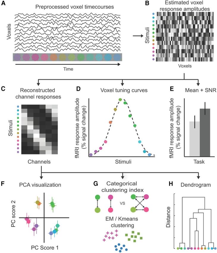
Schematic overview of the analysis procedure using simulated data. A, Voxel time courses were preprocessed (motion compensation, drift correction, high-pass filtering). B, Response amplitudes for each voxel were computed from the preprocessed voxel time courses, for each stimulus color, for each run, using linear regression (general linear model). C, Neural color space. A forward model (see Materials and Methods) was used to transform the data from the high-dimensional space of fMRI responses (dimensionality equal to the number of voxels) to a lower-dimensional space of six channels (each specified by a basis function for its color tuning curve). We refer to this six-dimensional space of channel responses as a neural color space; each stimulus color evokes a vector of six channel responses, i.e., a position in the six-dimensional space. The distances between colors in this space capture similarities between the corresponding patterns of activity. D, Voxel-based tuning curve. A von Mises function was fitted to the responses of each voxel to the 12 colors, separately for each task and visual area. The best-fit parameters of each tuning curve specified color preference, tuning width, and gain. E, Mean response and SNR. Response amplitudes were averaged across voxels, separately for each task and visual area. The SNR of each voxel was computed as the mean response of the voxel across stimulus colors divided by the SD across colors. The SNR of each visual area was computed by averaging SNRs across voxels. F, Two-dimensional visualization of the neural color space. The six-dimensional channel response matrices (C) were reduced by means of principal component analysis (PCA) to two dimensions for visualization. G, Clustering. The neural color spaces (C) were used to compute a categorical clustering index. The clustering index reflected the similarity between activity patterns evoked by stimulus colors within a perceptual category, compared to between-category colors. In addition, k-means and EM clustering algorithms were used to partition the neural color spaces into clusters. H, Hierarchical organization of the neural color space. The k-means and EM algorithms were used to compute hierarchical clustering, visualized by means of dendrograms.

fMRI experimental protocol.

Visual stimuli appeared for a duration of 1 s in a randomized order. Using an event-related design, interstimulus intervals ranged from 2 to 5 s, in steps of 1.5 s. All 12 colors were presented six times in each run, along with six blank trials. This created a total of 78 trials per run, with one run lasting ∼6 min. In the even-numbered runs, subjects performed an rapid serial visual presentation detection task continuously throughout each run. A sequence of white digits was displayed at fixation for 250 ms each, subtending ∼0.25° of visual angle with a luminance of 80 cd/m². The subject's task was to fixate the digits and indicate, by means of a button press, whether the current digit matched the one from two steps earlier. In the odd-numbered runs, subjects performed a color-naming task, using one of five buttons to indicate the most appropriate color name: one of the four unique hues (blue, red, yellow, green) or purple. In these runs, subjects were instructed to fixate a white fixation dot (luminance, 80 cd/m²; diameter 0.20°).

fMRI preprocessing.

fMRI data were preprocessed using standard procedures. The first four images of each run were discarded, allowing longitudinal magnetization to reach steady state. We compensated for head movements within and across runs using a robust motion estimation algorithm (Nestares and Heeger, 2000), divided the time course of each voxel by its mean image intensity to convert to percentage signal change and compensate for distance from the RF coil, and linearly detrended and high-pass filtered the resulting time course with a cutoff frequency of 0.01 Hz to remove low-frequency drift (Smith et al., 1999).

fMRI response amplitudes.

The response amplitudes to each color were computed separately for each voxel and separately for each run using linear regression. A regression matrix was constructed by convolving a canonical hemodynamic response function (HRF) and its numerical derivative with binary time courses (Friston, 2007) corresponding to the onsets of each of the 12 stimulus colors (with ones at each stimulus onset, and zeros elsewhere). The resulting regression matrix had 24 columns: 12 columns for the HRF convolved with each of the stimulus onsets and 12 columns for the HRF derivative. Response amplitudes were estimated by multiplying the pseudoinverse of this regression matrix with the preprocessed fMRI response time courses. We included the derivative because the HRF of an individual voxel may have differed from the canonical HRF (e.g., due to partial voluming with large veins). At least some of the response variability was captured by including the derivative; the variance of the estimated response amplitudes across runs was smaller with the derivative included than without it (Henson et al., 2002a,b; Brouwer and Heeger, 2009, 2011). The values obtained for the derivative regressors were discarded after response amplitudes were estimated, because we intended to have the derivates account only for differences in the timing of the responses, not the response amplitudes. We thus obtained, for each voxel and each run, one response amplitude for each of the 12 colors.

Voxel selection.

We selected a subset of voxels within each visual cortical area that showed the highest differential responses between colors. Specifically, we computed the ANOVA F statistic of response amplitudes across colors for each voxel. Voxels were included whose F statistic was above the 75th percentile of F statistics for voxels in each visual area. The 75th percentile split was arbitrary and used solely to select the most reliable voxels. A range of F statistic thresholds (25th to 75th percentile) yielded similar results and supported the same conclusions.

Normalization of response amplitudes.

Response amplitudes were normalized by removing a baseline from each voxel's response, separately for each run, in each scanning session. Specifically, let v be the number of voxels, and let s be the number of stimulus colors, giving us, for each run, a matrix of estimated response amplitudes B′ of size v × s. For each B′, we computed the mean voxel responses across all stimulus colors, yielding a vector m of mean response amplitudes of length v (one per voxel). This vector was normalized to a unit vector and removed by linear projection from the responses to each stimulus color: B = B′ − m(m^TB′).

Combining across sessions.

Measurements were combined across subjects and scanning sessions to increase sensitivity (Brouwer and Heeger, 2009, 2011). The estimated response amplitudes from a visual cortical area in a single session formed a v × n matrix, with v being the number of voxels (or dimensions) and n being the number of repeated measurements (one response amplitude for each color per run). In principle, sessions could have been combined in two ways. First, we could have concatenated the sessions, leaving the number of voxels (v) the same, but increasing the number of measurements (n). This would have required precise registration across sessions. We chose, instead, to stack the data sets, yielding a matrix B of size V × n, where V was the total number of voxels summed across sessions and subjects. We primarily present results from this “supersubject,” although we also report results from individual subjects.

Forward model.

We used a forward model (Brouwer and Heeger, 2009, 2011) to extract lower-dimensional neural color spaces from the spatially distributed patterns of voxel responses (Fig. 2). We characterized the color selectivity of each neuron as a weighted sum of six hypothetical channels, each with an idealized color tuning curve (or basis function) such that the transformation from stimulus color to channel outputs was one to one and invertible. Each basis function was a half-wave-rectified and squared sinusoid in DKL color space. We assumed that the response of a voxel was proportional to the summed responses of all the neurons in that voxel, and hence that the response tuning of each voxel was a weighted sum of the six basis function. To the extent that this is a reasonable approximation (Cardoso et al., 2012), it enabled us to estimate neural color spaces from the fMRI measurements. Data acquired with the diverted attention task (even runs) were analyzed separately from data acquired with the color-naming task (odd runs). Using leave-one-out validation, the measured voxel response amplitudes (B) were partitioned in training (B₁) and testing data sets (B₂). The training data were used to estimate the weights on the six hypothetical channels, separately for each voxel. With these weights in hand, we computed the channel responses associated with the spatially distributed pattern of activity across voxels in the test data. The estimated channel responses were stored as an n × c matrix C, where n was the number of stimulus colors (12), and c was the number of channels (6). A bootstrapping procedure was used to obtain a large number of channel response matrices C. On each iteration, we used a modified leave-one-out procedure that randomly selected one run to leave out for each session and then computed the channel responses C. Repeating this 100 times yielded 100 estimated channel response matrices for each task and visual area.

The channel responses C defined a six-dimensional neural color space for each visual area and each task condition. We used principal component analysis (PCA) previously to extract neural color spaces from the high-dimensional space of voxel responses (Brouwer and Heeger, 2009). In the current study, we instead used the forward model because it constrained the dimensionality reduction. The forward model was defined by six channels (idealized tuning functions) that respond to different colors in a circular color space. According to the model, each color produces a unique pattern of responses in the channels, represented by a point in the six-dimensional channel space. By fitting the voxel responses to the forward model, we projected the voxel responses into this six-dimensional subspace. Any covariation between or variation within voxels that could not be captured by the model (i.e., not in the subspace) was projected out. PCA, on the other hand, reduces dimensionality based on covariation between voxel responses, regardless of whether such covariation reflects color-selective signals or simply correlated noise unrelated to color. Neural color spaces extracted using PCA were qualitatively similar to those extracted with the forward model, but PCA yielded neural color spaces that were highly variable across runs, tasks, and visual areas. Compared to our previous work (Brouwer and Heeger, 2009), the current experimental protocol included more colors (12 instead of 8) and two separate task conditions, reducing the number of trials of each trial type. With fewer trials, correlated noise between voxels might have overwhelmed color-selective responses using PCA, while the constrained fit to the forward model was robust.

Visualization of color spaces.

To visualize the neural color spaces extracted using the forward model, we made two-dimensional plots of the color spaces using PCA. We computed the principal components for each channel response matrix C, and projected the channel responses onto the principal components creating a new n × c matrix S of principal component scores. The first two principal component scores for each color formed a coordinate pair, i.e., a location in a two-dimensional space, creating a two-dimensional plot of the neural color space that was easily visualized. PCA defined a two-dimensional plot that accounted for the greatest proportion of the variance in the six-dimensional channel responses C. The first two principal component scores accounted for almost all of the variance of the six-dimensional channel response matrix C (mean r² across visual areas and task conditions, 0.85). Reanalysis of our previously published data (Brouwer and Heeger, 2009) using this combination of the forward model (to reduce the dimensionality from the number of voxels to the number of channels) and PCA (to further reduce the dimensionality to two) yielded two-dimensional neural color spaces that were similar to those that we published previously using only PCA, supporting the same conclusions. Reanalysis of the current data using PCA to reduce dimensionality directly from the number of voxels to two also yielded two-dimensional neural color spaces that were similar to those published previously. Specifically, the neural color spaces from areas V4v and VO1 were close to circular, whereas the neural color spaces of the remaining areas (including V1) were not circular, replicating our previously published results and supporting the previously published conclusions (Brouwer and Heeger, 2009).

Categorical clustering index.

The neural color spaces (estimated channel responses C) were quantified in terms of categorical clustering, separately for each task and all visual areas. Categorical clustering quantified the extent to which the patterns of cortical activity evoked by within-category stimulus colors (e.g., shades of green) were more similar than patterns of activity evoked by between-category colors (e.g., blue vs yellow). We first calculated the distances between each color pair in the channel response matrices C. The clustering index was then computed as the average between-category distance divided by the average within-category distance. The statistical significance of differences in categorical clustering between tasks was computed using a nonparametric randomization test (explained in detail below). However, the most important statistical test was a comparison between the measured categorical clustering indices and the amount of clustering expected from a perfectly circular color space. This is because a circular space will already show some categorical clustering as color categories are formed by sets of neighboring colors within the space. For the current experiment, the baseline value for 12 colors and five categories was computed to be 2.27. A nonparametric test was used to determine whether the clustering indices were statistically greater than this baseline. Specifically, a distribution of clustering index values were computed for each of the 100 bootstrapped channel response matrices, separately for each task and visual area. Clustering was statistically significant if the baseline value was below the fifth percentile of this distribution of clustering indices (indicating 95% of the clustering indices computed for this visual area were above the baseline value of 2.27).

Expectation-maximization and k-means clustering.

In addition to our own clustering index, we used two complementary clustering algorithms to quantify the amount of categorical clustering in the neural color spaces: expectation-maximization (EM) clustering (Dempster et al., 1977) and k-means (MacQueen, 1967). k-means minimizes the sum, over all clusters, of the within-cluster sums of point-to-cluster-centroid distances. EM models each cluster as a multidimensional normal distribution. The input to both algorithms was the number of clusters that should be identified (five) as well as the 100 bootstrapped channel response matrices C. Thus, for each visual area and task, the input constituted a matrix of n × 6 points, where n = 1200 was the number of colors (12) times the number of bootstrapped channel response matrices (100). The output of both algorithms was an n element vector indicating cluster membership. The correspondence between EM clustering and perceptual clustering was quantified using the adjusted Rand index (Rand, 1971; Hubert and Arabie, 1985). This index computed the fraction of the 1200 reconstructed channel responses for which the algorithm placed the stimulus color in the correct psychophysical color category. Without adjustment, the Rand index is bounded between 0 (no correspondence) and 1 (complete correspondence). However, this does not take into account that random groupings will produce some correspondence just by chance. The chance value was used to adjusted the Rand index, making it take on a value of 0 for Rand indices expected by chance (Hubert and Arabie, 1985). A high value for the adjusted Rand index indicated a close correspondence between perceptual categories and clustering within the neural color space. The statistical significance of differences in adjusted Rand indices between tasks was computed using a nonparametric randomization test (see “Statistics” below).

Like the categorical clustering measure, the Rand indices were compared to a baseline index computed from a perfectly circular neural color space. Strictly speaking, a circular color space consists of 12 separate clusters (one for each stimulus color) with equidistant spacing from each other. There is no optimal way of grouping these 12 separate clusters into a smaller set of five category clusters. The EM clustering algorithm is initialized with random assignments of colors to clusters, consequently returning a different random clustering on each iteration. However, the EM algorithm tends to group nearby colors from a perfectly circular color space, resulting in an inflated Rand index. We thus compared the observed adjusted Rand index values with a null distribution of Rand indices computed from a perfectly circular color space. This null distribution was created using a Monte Carlo simulation: we repeatedly (1000 times) ran the EM clustering algorithm (initialized each time with random starting weights) on a perfectly circular color space and computed the resulting adjusted Rand index. The percentage of this null distribution greater than the actually observed Rand index value was designated as the (one-tailed) p value.

Hierarchical clustering.

We used both the EM algorithm and k-means to compute hierarchical clusterings, and to compare color-category hierarchies between the neural and perceptual color spaces. We computed a distance matrix between the channel responses evoked by each color pair and transformed it into a dendrogram (a cluster tree) in which the height of each pair of branches represented the distances between clusters. A similar dendrogram was computed from the psychophysical data, based on the frequency with which subjects placed two colors in the same category. Short distances in the dendrogram corresponded to pairs of colors that were always placed in the same category bin.

Mean response amplitudes, SNR, and goodness of fit.

Mean response amplitudes were computed by averaging the responses across voxels, runs, and subjects, separately for each visual cortical area and task condition (diverted attention, color naming). Signal-to-noise ratios (SNRs) were computed by calculating the mean response amplitude for each voxel (averaged across color and runs) and dividing by the SD of the responses (across colors and runs). The SNRs were then averaged across voxels, sessions, and subjects, separately for each visual cortical area and task condition. We also computed the goodness of fit of the GLM model to each voxel's response time course (r²). The statistical significance of differences in mean response amplitudes, SNR, and goodness of fit between tasks was computed using a nonparametric randomization test (see below).

Voxel tuning curves: gain, offset, and tuning width.

We fitted voxel-based tuning curves to the normalized response amplitudes, separately for each voxel, using von Mises functions (Jammalamadaka and Sengupta, 2001): f(x|μ, k) = [exp(k × [cos(x − μ)])/[2 × π × I₀(k)] × g] + b, where the values of x corresponded to the stimulus colors. The free parameters of this function are μ (preferred direction in color space), k (tuning width), g (gain), and b (offset). I₀(k) is the modified Bessel function of order 0. Nonlinear least squares fitting was used to estimate the parameters for each voxel to the 12 colors, separately for each task and separately for each subject and scanning session, but averaged across runs within a scanning session. For each visual area, we then computed the median of these parameter estimates and took the reciprocal of the k parameter to transform it to a more intuitive measure of tuning width (in degrees) at half maximum. The statistical significance of differences in gain and tuning width between tasks was computed using a nonparametric randomization test (see “Statistics” below).

Statistics.

The differences between tasks in the various measures outlined above (categorical clustering, adjusted Rand indices, mean response amplitudes, SNR, goodness of fit, voxel-based tuning gain, and voxel-based tuning width) were all analyzed using the same nonparametric randomization test. For each of these measures, we obtained a null distribution for the difference between tasks (color naming, diverted attention), separately for each visual area. This null distribution was created by randomly shuffling the task labels (color naming, diverted attention) a large number of times (1000) and recomputing after each reshuffling the resulting mean for each task. The measured difference value was then compared with this null distribution; the proportion of the null distribution greater than the measured value was designated as the (one-tailed) p value. We preferred this approach over more conventional parametric methods (e.g., two-way ANOVA), as we had no reason to assume that these measures were distributed normally, or that variances were comparable across tasks. However, a two-way ANOVA supported the same conclusions to those reached using the nonparametric randomization test. Unlike an ANOVA, the nonparametric randomization test does not provide a single summary statistic for all comparisons (differences in measures between tasks across all visual areas). Instead, each visual area is associated with a its own statistical significance. To simplify and reduce clutter, we report the largest p value found across visual areas for each measure.

MRI acquisition.

MRI data were acquired with a Siemens 3T Allegra head-only scanner using a head coil (NM-011; NOVA Medical) for transmitting and an eight-channel phased array surface coil (NMSC-021; NOVA Medical) for receiving. Functional scans were acquired with gradient recalled echoplanar imaging to measure blood oxygen level-dependent changes in image intensity (Ogawa et al., 1990). Functional imaging was conducted with 24 slices oriented perpendicular to the calcarine sulcus and positioned with the most posterior slice at the occipital pole (repetition time, 1.5 s; echo time, 35 ms; flip angle, 75°; 2.0 × 2.0 × 2.5 mm; 104 × 80 grid size). A T1-weighted magnetization-prepared rapid gradient echo (MPRAGE; 1.5 × 1.5 × 3 mm) anatomical volume was acquired in each scanning session with the same slice prescriptions as the functional images. This anatomical volume was aligned using a robust image registration algorithm (Nestares and Heeger, 2000) to a high-resolution anatomical volume. The high-resolution anatomical volume, acquired in a separate session, was the average of several MPRAGE scans (1 × 1 × 1 mm) that were aligned and averaged, and used not only for registration across scanning sessions, but also for gray matter segmentation and cortical flattening (see below).

Defining visual cortical areas.

Visual cortical areas were defined using standard retinotopic mapping methods (Engel et al., 1994, 1997; Sereno et al., 1995; Larsson and Heeger, 2006), with the exact procedure described in detail previously (Brouwer and Heeger, 2009, 2011). There is some controversy over the definition of human V4 and the areas just anterior to it (Tootell and Hadjikhani, 2001; Hansen et al., 2007). We adopted the convention of defining V4v, VO1, and VO2 as adjacent visual cortical areas on the ventral surface of the occipital lobe, each with a representation of the entire contralateral hemifield (Brewer et al., 2005; Wandell et al., 2007). We defined the ROIs conservatively, avoiding the boundaries (reversals) between adjacent visual field maps, to reduce the risk of assigning a voxel to the wrong visual cortical area. Area hMT+ (the human MT complex) was defined, using data acquired in a separate scanning session, as an area in or near the dorsal/posterior limb of the inferior temporal sulcus that responded more strongly to coherently moving dots relative to static dots (Tootell et al., 1995a,b), setting it apart from neighboring areas LO1 and LO2 (Larsson and Heeger, 2006).

Results

Psychophysics

Given five color categories in which to place 64 stimulus colors, subjects were consistent where they placed category boundaries (Fig. 3). The most stable categories were “green” and “blue.” Four of five subjects separated the darker purples and the brighter magentas/pinks into two different categories (although they varied somewhat in the boundary location between the categories), whereas they combined the orange and yellow stimulus colors into a single category. The remaining subject (S1) combined all mixtures of red and blue into a single category, but separated the orange and yellow stimuli into two distinct categories. Averaging across subjects, the five categories used for the analysis of the subsequent fMRI measurements were “blue” (including 3 of 12 colors in the fMRI experiment), “purple” (2 of 12 colors), “magenta/pink” (2 of 12 colors), “yellow” (2 of 12 colors), and “green” (3 of 12 colors).

Figure 3.

Psychophysics: color categorization. First row, Twelve stimulus colors used in the fMRI experiments. Second row, Sixty-four colors (taken from the same circular color space as the 12 colors in the first row) used in the psychophysics experiment. Rows S1, S2, S3, S4, and S5 represent the category boundaries for each subject, respectively. Subjects were asked to partition the 64 stimulus colors into five bins, according to what they felt was a natural division of the continuous color space into five categories. The color representing each category is the average of all the colors that the subject included in the category.

Greater categorical clustering in V4v and VO1 for color naming

We extracted neural color spaces from the fMRI measurements, separately for each visual area and each task condition (diverted attention vs color naming). In each of these low-dimensional neural color spaces, the distances between each pair of stimulus colors represented the similarity between the patterns of activity evoked by the colors.

Clustering of the within-category colors was evident in the neural color spaces, particularly in VO1 and V4v, and particularly for the color-naming task (Fig. 4A,B; visualized in 2D using PCA; see Materials and Methods). In contrast, the neural color space extracted from neighboring visual area V3 was largely circular and therefore low in categorical clustering (Fig. 4C). To quantify these results, we computed an index of categorical clustering from distances between pairs of colors (Fig. 5A). The key test of categorical clustering was the comparison of the clustering index with a baseline value corresponding to a perfectly circular neural color space (see Materials and Methods). Below this baseline, any change in the index value confounds categorical clustering with circularity of the neural color space. The clustering indices were significantly greater than the baseline value only areas V4v and VO1, and only for the color-naming task (nonparametric randomization test, p < 0.001). The categorical clustering indices in all other visual areas fell short of this baseline.

Figure 4.

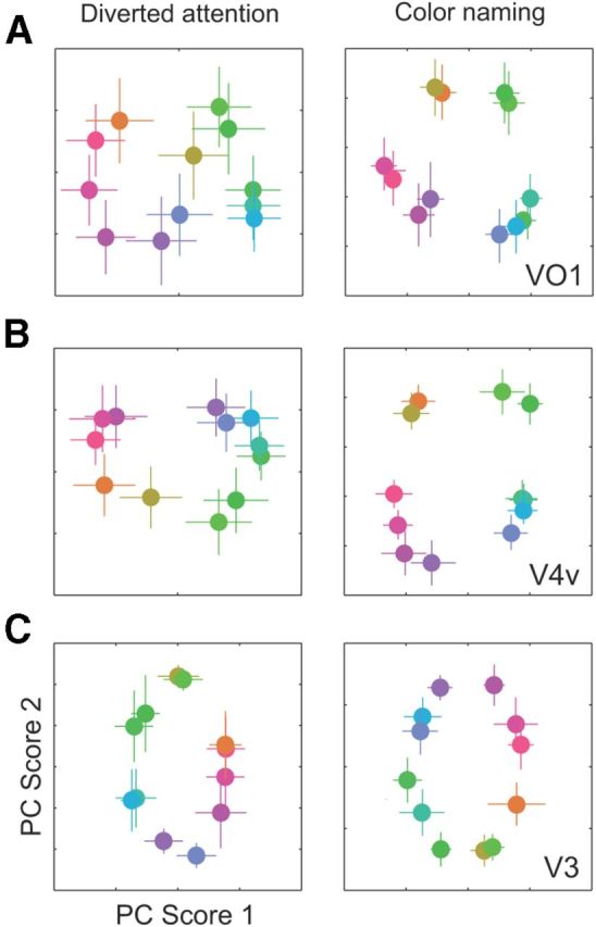
Categorical clustering in neural color spaces. A, Visual area VO1. B, V4v. C, V3. Left, Diverted attention task. Right, Color-naming task. Channel responses were estimated from the fMRI measurements using the forward model and visualized in 2D plots using principal component analysis. Coordinates of each stimulus color in the plots correspond to the first two principal component scores of the channel responses (see Materials and Methods). Each individual point is the mean coordinate averaged across 100 bootstrapped estimates of the channel responses (see Materials and Methods). Errors bars represent the horizontal and vertical SDs of each coordinate.

Figure 5.

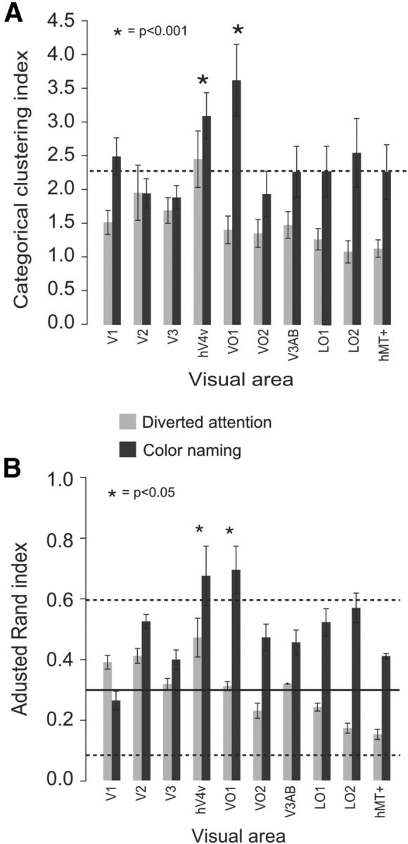
Color-category specific clustering. A, Categorical clustering indices for each visual area and for each of the two task conditions. Light gray bars, Diverted attention task; dark gray bars, color-naming task; dashed line, baseline categorical clustering index for a perfectly circular color space that shows no clustering at all. Asterisks indicate visual areas/tasks for which the index was significantly greater than expected from a circular color space. Error bars indicate the SD in clustering across bootstrapped channel responses. B, Adjusted Rand indices for each visual area and each task (same format as in A). The adjusted Rand index quantifies the correspondence between clustering in the neural color spaces and the perceptual categories. The solid line indicates the mean of the baseline distribution of adjusted Rand indices for a perfectly circular color space that shows no clustering at all, computed using a Monte Carlo simulation. The dashed lines indicate the 5th and 95th percentiles for the baseline distribution. Asterisks indicate visual areas/task for which the index was significantly greater than expected from a circular color space. Error bars indicate the SD in the adjusted Rand indices computed across bootstrapped channel responses.

The categorical clustering indices were significantly larger for color naming than diverted attention in all but one (V2) visual area (p < 0.001, nonparametric randomization test), but the difference between color naming and diverted attention was significantly greater in VO1 relative to the other visual areas (p < 0.01, nonparametric randomization test). One possibility is that all visual areas exhibited clustering of within-category colors, but that the categorical clustering indices were low in visual areas with fewer color-selective neurons, i.e., due to a lack of statistical power. Another possibility is that the increase in categorical clustering index observed in areas other than V4v and VO1 solely reflected an increase in the circularity of the color spaces, but no increase in clustering. To distinguish between these two possibilities would require considerably larger data sets to gain statistical power or other methods capable of isolating the responses of a large number of color-selective neurons in each visual area.

Categorical clustering in area V4v was close to baseline (i.e., close to that expected for a perfectly circular color) for the diverted attention task, replicating our earlier findings (Brouwer and Heeger, 2009). But no visual area exhibited categorical clustering significantly greater than baseline for the diverted attention task.

Color sensitivity in the retina varies as a function of location, most notably the increase in S-cones as a function of eccentricity, and the complete absence of S-cones in central fovea. We previously reported a lack of a systematic shift in a classifier's ability to distinguish between different colors as function of eccentricity (Brouwer and Heeger, 2009). Similarly, we found no significant change in categorical clustering as a function of eccentricity in the current experimental data.

Clustering in V4v and VO1 resembled perceptual color categories

Clustering in the neural color spaces was similar to that measured psychophysically. Qualitatively, the only discrepancy we found between the neural color spaces and the psychophysical categories was that the turquoise/cyan stimulus color in the neural spaces was grouped with the blues, while psychophysically, this stimulus color was placed in the green category. We used a standard clustering algorithm, EM clustering, to quantify the comparison. The algorithm was used to partition the neural color spaces into five clusters. We then compared this clustering with the psychophysical categories using the adjusted Rand index (see Materials and Methods; Fig. 5B). A high value for the adjusted Rand index indicated a close correspondence between perceptual categories and clustering within the neural color space. Only for the color-naming task, and only in V4v and VO1, were the adjusted Rand index values statistically greater than the baseline Rand index expected from a perfectly circular color space (p < 0.01, nonparametric Monte Carlo simulation; see Materials and Methods). These results were highly similar to those obtained using k-means (data not shown), a different but widely used clustering algorithm, as well as our own clustering index.

Hierarchical clustering in areas V4v and VO1 resembled the perceptual hierarchy of color categories

We used the EM algorithm to compute a hierarchical organization of the neural color spaces and to compute a hierarchical organization of perceptual color categories. The resulting dendrograms (cluster trees) extracted from VO1 (Fig. 6B) and V4v (data not shown) for the color-naming task resembled the dendrogram extracted from the psychophysical measurements (Fig. 6C). In these dendrograms, the height of each pair of branches represents the similarity between the two colors being connected, as measured by the frequency with which these colors were placed in the same cluster. The VO1 dendrogram for the color-naming task revealed seven different categories at the lowest level of the hierarchy (Fig. 6B): two greens, two turquoise colors, cyan, blue, two purples, two magentas, and yellow/orange. At the next level, these were combined into three categories: green/yellow, blue/turquoise, and magenta/purple, each containing four of the 12 stimuli. The psychophysical color category judgments exhibited a similar dendrogram (Fig. 6C), with two exceptions: (1) the turquoise color was not consistently placed in the green category (evident at the lowest level of the dendrogram), and (2) the VO1 hierarchy combined greens and yellows before combining these with blues and purples, whereas the psychophysical hierarchy combined greens and blues before combing these with purples/magenta and yellows. In contrast, the VO1 dendrogram for the diverted attention task (Fig. 6A) exhibited only weak correspondence with perceptual dendrogram. The V4v dendrograms were very similar to those extracted from VO1. None the dendrograms extracted from any of the other visual areas, for either task, were similar to the perceptual dendrogram.

Figure 6.

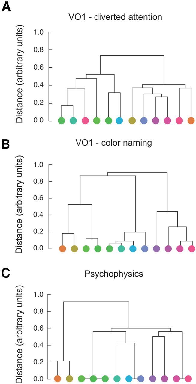
Hierarchical clustering. A, Dendrogram extracted from VO1 activity during the diverted attention task. The height of each pair of branches in the dendrogram (cluster tree) represents the similarity between the patterns of activity evoked by the two colors being connected. B, Dendrogram extracted from VO1 activity during the color-naming task. C, Dendrogram extracted from color categorization psychophysics (see Fig. 2). The height of each pair of branches represents the relative frequency with which subjects placed the two stimulus colors in the same category.

Response amplitudes, SNR, voxel-based tuning curves, and model fits

Mean response amplitudes were larger for the color-naming task in all visual areas (p < 0.001, nonparametric randomization test; Fig. 7A). However, there were no significant differences in mean responses amplitudes between different stimulus colors. Apart from differences in response amplitudes, the temporal dynamics of evoked responses were not significantly different between tasks. We fitted the event-related responses, averaged across voxels, to a canonical hemodynamic response function with six free parameters (Friston, 2007). We found no significant differences in the estimated parameters between tasks (p > 0.50, nonparametric randomization test).

Figure 7.

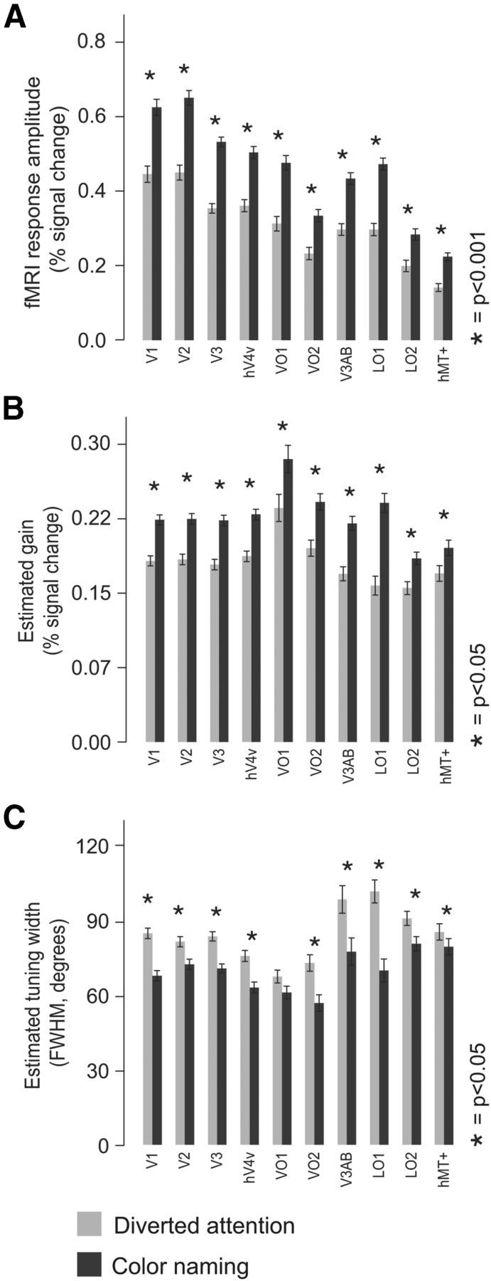
Response amplitudes, gain, and voxel tuning width. A, Response amplitudes, averaged across all voxels within each visual area, for each of the two task conditions. Light gray bars, Diverted attention task; dark gray bars, color-naming task. Error bars indicate SDs across subjects and scanning sessions. Asterisks indicate visual areas for which the responses were significantly greater during the color-naming task compared to the diverted attention task. B, Estimated gain in each visual, for each task. Error bars indicate SDs across subjects and scanning sessions. C, Estimated average tuning width (full-width at half maximum, in degrees) for each visual area and for each task. Error bars indicate SDs across subjects and scanning sessions.

The larger response amplitudes were accompanied by greater SNR. We computed SNR, separately for each voxel, as the ratio between the mean response amplitude and SD across repeated stimulus presentations, and then averaged across voxels in each visual area. The SNR was greater for color naming in most visual areas (V2, V3, V4v, VO1, LO1, LO2, and MT+: p < 0.05, nonparametric randomization test; V1, p = 0.51; VO2, p = 0.47). Converging evidence for greater SNR was observed by comparing the goodness of fit to each voxel's response time course (r²; see Materials and Methods). The r² values were significantly greater for the color-naming task in all visual areas (p < 0.01, nonparametric randomization test).

The larger response amplitudes were accompanied by narrower voxel-based tuning curves and greater response gains. We fitted the responses of each voxel to a circular Gaussian tuning curve (see Materials and Methods) separately for each task, and then averaged the fitted parameter values across voxels in each visual area. The gains of the best-fit tuning curves were greater for the color-naming task in all visual areas (p < 0.01, nonparametric randomization test). In addition, tuning widths were narrower in all visual areas (p < 0.01, nonparametric randomization test), with exception of areas VO1 (p = 0.053) and hMT+ (p = 0.45).

How much of the response variability in the voxels was captured by the forward model? After computing the forward model weights (see Materials and Methods), we created a matrix of predicted voxel responses, given the weights and the forward model. We then calculated the fit (r²) between these predicted and the actual voxel responses, separately for each visual area and task. This revealed a significant increase in the model fit during the color-naming task in all visual areas (p < 0.0001), with the exception of area V3, which showed a significant decrease (p < 0.001). The best fit between the forward model and data was observed in V4v, in both tasks, while the biggest increase in fit quality was observed in area VO1, where the model fit almost doubled during color naming. The r² values were not very high (ranging from 0.05 for area MT+ to 0.12 for area V4v), however, raising concern that the forward model might have failed to characterize responses of color-selective neurons. Previously, we demonstrated that stimulus color could be decoded from the evoked responses using either the (same) forward model or a maximum likelihood classifier (Brouwer and Heeger, 2009). Decoding accuracies with the forward model and classifier were indistinguishable from one another (r = 0.94). Decoding accuracies from the current data set were similar; forward-model decoding and maximum-likelihood decoding and were nearly indistinguishable. This suggests that the residuals not captured by the forward model constituted primarily measurement and/or physiological noise because there was little, if any, information about color in the residuals not captured by the forward model.

One possible concern is that areas VO1 and V4v exhibited categorical clustering, even during the diverted attention task, but that we could only observe such categorical clustering during the color-naming task because it was associated with higher SNR. Therefore, in a separate analysis, we selectively reduced the SNR associated with the color-naming task by removing voxels with high SNR and repeating the analysis. Specifically, we removed the voxels with r² values above the 50th, 60th, 70th, 80th, and 90th percentiles. Removing these high SNR voxels from the color-naming task data had a dramatic effect on the average SNR, and even removing the best 10% of voxels reduced the average SNR of the color-naming task such that it was no longer significantly different from the average SNR in the diverted attention task. The categorical clustering measure was largely unaffected by reducing SNR: areas V4v and VO1 continued to show significant clustering during the color-naming task, while the other visual areas did not, even with 50% of the best voxels removed from each visual area.

Individual subjects

These results were evident also in individual subjects. Mean response amplitudes and SNRs were greater for color naming in most visual areas and most individual subjects. For example, response amplitudes from V4v were larger for color naming in four of five subjects, and from VO1 in four of five subjects (p < 0.001, nonparametric randomization test). Categorical clustering from VO1 and V4v was numerically greater during color naming in all five subjects, but the clustering index and Rand index values were statistically greater than baseline for only one of five subjects (p < 0.05, nonparametric randomization test). This likely reflects a limitation in measuring response amplitudes precisely in the presence of physiological and instrumentation noise.

Given that the clustering index values were not statistically significant in each subject individually, we were concerned that the results, when combined across subjects, might rely mostly on a subset of the subjects. We therefore repeated the same analyses described above, combining across subjects, but leaving one subject out in turn. The results obtained in this way were similar to those obtained by combining all subjects, and supported the same conclusions, regardless of which subject was left out.

A neural model of categorical clustering

We propose a model for how a categorical representation of color can be induced by changes in the gain of color-selective neurons. The proposed gain changes are similar to those observed during spatial and feature-based attention tasks. In the model, color is encoded by the activity of many neurons, each tuned to a different hue. During the diverted attention task (or during passive viewing), the maximum firing rates of all these neurons are similar (Fig. 8A), and, consequently, the low-dimensional (2D) neural color space extracted from the activity of these neurons is circular (Fig. 8B). When subjects are actively attending to the color stimuli, we propose that there is an increase in gain for all color-selective neurons across all visual cortical areas. Such an increase in gain is hypothesized to cause the observed increases in response amplitudes and SNR (assuming that the noise is additive). We verified through model simulations that the neural color space is not affected by this nonspecific gain increase. We also verified that the neural color space is not affected by an additive increase in baseline responses.

Figure 8.

A neural model for categorical clustering. A, Color is represented by the activity of broadly tuned neurons, each with a different preferred color. Each black curve is a simulated tuning curve. For the diverted attention task, all neurons have the same gain (peak height of the tuning curves). B, Circular neural color space extracted from the simulated responses in A. C, For the color-naming task, responses from some visual areas (e.g., V4v and VO1) are enhanced, but only for neurons that prefer colors near the category centers (e.g., red, green, blue, yellow). D, Neural color space extracted from the simulated responses in C, showing categorical clustering.

To model the transformation (i.e., clustering) in the neural color space, we propose that some visual areas (e.g., V4v and VO1) implement an additional color-specific change in gain, such that the gain of each neuron changes as a function of its selectivity relative to the centers of the color categories (Fig. 8C). Specifically, neurons tuned to a color near the center of a color category are subjected to larger gain increases than neurons tuned to intermediate colors. This color-specific gain change mimics the responses of macaque IT neurons observed when monkeys perform a color categorization task (Koida and Komatsu, 2007). The resulting neural color space, with color-specific gain modulations, exhibits clustering (Fig. 8D).

This model predicts narrower voxel-based tuning curves with color-specific gain increases, as observed in our data for the color-naming task. Each voxel contains a large number of neurons with a wide range of color preferences. The voxel-based tuning curves depend on the distributions of color preferences, response gains, and tuning widths of all of the neurons in each voxel. If the gain increases for only one subpopulation of neurons (all with the same preferred color), with no change in neural tuning widths, then the voxel-based tuning curves will appear to have both higher gain and narrower tuning. A similar prediction follows from increasing the gains of several subpopulations of neurons, each subpopulation with a different preferred color.

The model also predicts that the response gains of each voxel should differ, depending on the distance from its preferred color to color-category centroids. We did not find significant differences in gain dependent on the preferred color of each voxel. There was only a weak correlation between distance and gain in area V4v for color naming. We suspect that our measurements lacked the necessary statistical power to test this prediction. In addition, the choice of stimuli may not have included a sufficiently large number of colors sampling hue densely enough to reveal the hypothesized color-selective changes in gain. A related prediction of the model is that mean response amplitudes (averaged across voxels) should depend on stimulus color, with colors near the category centroids evoking the largest responses for the color-naming task. We did not observe evidence for this prediction, but again the statistical power in our measurements may have been limited by not sampling hue densely enough.

Discussion

Categorical clustering of neural representation of color in V4v and VO1

Task-dependent modulations of activity are readily observed throughout visual cortex, associated with spatial attention, feature-based attention, perceptual decision making, and task structure (Kastner and Ungerleider, 2000; Treue, 2001; Corbetta and Shulman, 2002; Reynolds and Chelazzi, 2004; Jack et al., 2006; Maunsell and Treue, 2006; Reynolds and Heeger, 2009). These task-dependent modulations have been characterized as shifting baseline responses, amplifying gain and increasing SNR of stimulus-evoked responses, and/or narrowing tuning widths.

The focus in the current study, however, was to characterize task-dependent changes in distributed neural representations, i.e., the joint encoding of a stimulus by activity in populations of neurons. We measured distributed patterns of fMRI responses to color and computed neural color spaces from these measurements. Neural color spaces from areas V4v and VO1 showed significant categorical clustering for the color-naming task, but not for the diverted attention task. These were the only visual areas that exhibited clustering, although we observed significantly larger response amplitudes and greater signal-to-noise ratios in all visual areas for color naming. When subjects engaged in color naming, the neural representations of color in V4v and VO1 were transformed, making patterns of activity of within-category colors more similar, while making patterns of activity of between-category colors more dissimilar. The clustering was similar to the subjective perception of color categories, thus revealing a neural correlate of perceptual color categories in human visual cortex.

Categorical specificity of areas V4v and VO1

A multitude of studies have shown that both human and macaque V4 and adjacent areas respond strongly and selectivity to chromatic stimuli (Zeki, 1973; Hadjikhani et al., 1998; Bartels and Zeki, 2000; Wade et al., 2002; Brewer et al., 2005; Conway and Tsao, 2006; Conway et al., 2007; Koida and Komatsu, 2007; Stoughton and Conway, 2008; Wade et al., 2008; Brouwer and Heeger, 2009). We showed previously that the neural representation of color in V4v and adjacent area VO1 (during a similar, but less demanding diverted attention task to that used in the current study) better matched our perceptual experience of color, compared to other visual areas (Brouwer and Heeger, 2009). However, few studies have investigated the neural representation of color categories, the representation of the unique hues, or the effect of task demands on these representations.

Previous evidence for a potential categorical representation in the visual system comes from the observation that although macaque IT neurons are tuned to all directions in color space, the distribution is not uniform. Rather, the population distribution contains three prominent peaks in color tuning, aligned with the unique hues red, green, blue, and, to a lesser extent, yellow (Stoughton and Conway, 2008). In addition, changes in the response properties of color-selective neurons as a result of task demands have been observed in macaque IT. When animals were rewarded for categorizing a stimulus as being either green or red, color signals differentiating these two colors were enhanced, although color selectivity was conserved (Koida and Komatsu, 2007).

Neural correlates of color categories have also been identified in the human brain using EEG. Specifically, successive within-category colors change the amplitude and latency of the event-related potential components associated with the perceived mismatch between the current visual input (i.e., a shade of green) and preceding stimuli (i.e., different shades of green), relative to successive presentations of between-category colors (Fonteneau and Davidoff, 2007; Liu et al., 2009; Thierry et al., 2009; Mo et al., 2011). Furthermore, the effects appear to be lateralized, providing support for the influence of language on color categorization, the principle of linguistic relativity, or Whorfianism (Hill and Mannheim, 1992; Liu et al., 2009; Mo et al., 2011). Indeed, language-specific terminology influences preattentive color perception. The existence in Greek of two additional color terms, distinguishing light and dark blue, leads to faster perceptual discrimination of these colors and an increased visual mismatch negativity of the visually evoked potential in native speakers of Greek, compared to native speakers of English (Thierry et al., 2009).

In the current study, we took a step further and derived, from our fMRI measurements, the underlying neural representations (i.e., the neural color spaces), and found evidence for categorical clustering, but only when subjects were performing the color-naming task. Unlike the previous EEG study, however, we found no evidence of lateralized categorical clustering: clustering was statistically significant for V4v and VO1 in both hemispheres, and not significantly different between hemispheres (data not shown).

Macaque versus human color vision

There is a continuing debate on the relationship between human V4v and macaque V4. Whereas some have argued that human V4 consists of a dorsal and ventral part (V4v and V4d) (Hansen et al., 2007), differences in retinotopy and functional properties suggest that these two human cortical regions are distinct. Unlike V4v, putative human V4d does not respond more strongly to color than to grayscale stimuli (Tootell and Hadjikhani, 2001; Wade et al., 2002, 2008; Winawer et al., 2010; Goddard et al., 2011). Macaque V4v (adjacent to V3v) and V4d (adjacent to V3d) represent complementary parts of the contralateral hemifield. In humans, on the other hand, V4v (adjacent to V3v) and LO1 (adjacent to V3d) each contain representations of the entire contralateral hemifield (Press et al., 2001; Larsson and Heeger, 2006; Bridge and Parker, 2007; Swisher et al., 2007). In further support of this distinction, we did not find significant categorical clustering in LO1 and LO2, although the clustering values from these areas were consistently higher than those from neighboring areas hMT+ and V3AB. Instead, we found significant categorical clustering only in the ventral visual areas V4v and VO1.

This is also cause for caution, in general, when comparing the pathways of color vision between species. Color perception might differ between humans and macaques. Macaque and human photoreceptors differ in their spectral sensitivities (Kaiser and Boynton, 1996), as do the proportions of long-, middle-, and short-wavelength photoreceptors (Dobkins et al., 2000). Despite these differences, it is reasonable to hypothesize that the same computational processes underlie the transformations in neural representations across the hierarchy of visual areas, in both species.

A neural model of color categorization

We proposed a model that explains the clustering of the neural color spaces from V4v and VO1, as well as the changes in response amplitudes (gain) and SNR observed in all visual areas. In this model, the categorical clustering observed in V4v and VO1 is attributed to a color-specific gain change, such that the gain of each neuron changes as a function of its selectivity relative to the centers of the color categories.

Our study was not designed to distinguish between the possible contributions of spatial and featural attention to these gain changes. The diverted attention task required subjects to attend at fixation, and the color-naming task required them to attend instead to the peripheral locations of the colored stimuli, confounding any change in featural attention with the change in spatial attention. If color-selectivity varies with eccentricity, then the shift in spatial attention alone (with no change in featural attention) might have caused color-specific gain changes. However, both the present study and a previous one (Brouwer and Heeger, 2009) found no evidence for differences in color-selectivity as a function of eccentricity. Consequently, the change in categorical clustering for the color-naming task was likely dominated by featural attention. Although the origin of neural signals responsible for adjusting the gains of the color-selective neurons is beyond the scope of the current study, other research suggests that neural activity in prefrontal cortex encodes task-specific rules (Miller and Cohen, 2001).

References

- Bartels A, Zeki S. The architecture of the colour centre in the human visual brain: new results and a review. Eur J Neurosci. 2000;12:172–193. doi: 10.1046/j.1460-9568.2000.00905.x. [DOI] [PubMed] [Google Scholar]
- Brainard D. Cone contrast and opponent modulation color spaces. In: Kaiser PK, Boynton RM, editors. Human color vision. Washington, DC: Optical Society of America; 1996. pp. 563–579. [Google Scholar]
- Brewer AA, Liu J, Wade AR, Wandell BA. Visual field maps and stimulus selectivity in human ventral occipital cortex. Nat Neurosci. 2005;8:1102–1109. doi: 10.1038/nn1507. [DOI] [PubMed] [Google Scholar]
- Bridge H, Parker AJ. Topographical representation of binocular depth in the human visual cortex using fMRI. J Vis. 2007;7(14):15, 11–14. doi: 10.1167/7.14.15. [DOI] [PubMed] [Google Scholar]
- Brouwer GJ, Heeger DJ. Decoding and reconstructing color from responses in human visual cortex. J Neurosci. 2009;29:13992–14003. doi: 10.1523/JNEUROSCI.3577-09.2009. [DOI] [PMC free article] [PubMed] [Google Scholar]
- Brouwer GJ, Heeger DJ. Cross-orientation suppression in human visual cortex. J Neurophysiol. 2011;106:2108–2119. doi: 10.1152/jn.00540.2011. [DOI] [PMC free article] [PubMed] [Google Scholar]
- Cardoso MM, Sirotin YB, Lima B, Glushenkova E, Das A. The neuroimaging signal is a linear sum of neurally distinct stimulus- and task-related components. Nat Neurosci. 2012;15:1298–1306. doi: 10.1038/nn.3170. [DOI] [PMC free article] [PubMed] [Google Scholar]
- Conway BR, Tsao DY. Color architecture in alert macaque cortex revealed by FMRI. Cereb Cortex. 2006;16:1604–1613. doi: 10.1093/cercor/bhj099. [DOI] [PMC free article] [PubMed] [Google Scholar]
- Conway BR, Moeller S, Tsao DY. Specialized color modules in macaque extrastriate cortex. Neuron. 2007;56:560–573. doi: 10.1016/j.neuron.2007.10.008. [DOI] [PMC free article] [PubMed] [Google Scholar]
- Corbetta M, Shulman GL. Control of goal-directed and stimulus-driven attention in the brain. Nat Rev Neurosci. 2002;3:201–215. doi: 10.1038/nrn755. [DOI] [PubMed] [Google Scholar]
- Corbetta M, Miezin FM, Dobmeyer S, Shulman GL, Petersen SE. Attentional modulation of neural processing of shape, color, and velocity in humans. Science. 1990;248:1556–1559. doi: 10.1126/science.2360050. [DOI] [PubMed] [Google Scholar]
- Dean P. Visual cortex ablation and thresholds for successively presented stimuli in rhesus monkeys: II. Hue. Exp Brain Res. 1979;35:69–83. doi: 10.1007/BF00236785. [DOI] [PubMed] [Google Scholar]
- Dempster AP, Laird NM, Rubin DB. Maximum likelihood from incomplete data via EM algorithm. J Roy Stat Soc B Met. 1977;39:1–38. [Google Scholar]
- Derrington AM, Krauskopf J, Lennie P. Chromatic mechanisms in lateral geniculate nucleus of macaque. J Physiol. 1984;357:241–265. doi: 10.1113/jphysiol.1984.sp015499. [DOI] [PMC free article] [PubMed] [Google Scholar]
- Dobkins KR, Thiele A, Albright TD. Comparison of red-green equiluminance points in humans and macaques: evidence for different L:M cone ratios between species. J Opt Soc Am A Opt Image Sci Vis. 2000;17:545–556. doi: 10.1364/JOSAA.17.000545. [DOI] [PubMed] [Google Scholar]
- Engel SA, Rumelhart DE, Wandell BA, Lee AT, Glover GH, Chichilnisky EJ, Shadlen MN. fMRI of human visual cortex. Nature. 1994;369:525. doi: 10.1038/369525a0. [DOI] [PubMed] [Google Scholar]
- Engel SA, Glover GH, Wandell BA. Retinotopic organization in human visual cortex and the spatial precision of functional MRI. Cereb Cortex. 1997;7:181–192. doi: 10.1093/cercor/7.2.181. [DOI] [PubMed] [Google Scholar]
- Farnsworth D. Manual: the Farnsworth Munsell 100 hue test for the examination of discrimination. Baltimore: Munsell Colour; 1957. [Google Scholar]
- Fonteneau E, Davidoff J. Neural correlates of colour categories. Neuroreport. 2007;18:1323–1327. doi: 10.1097/WNR.0b013e3282c48c33. [DOI] [PubMed] [Google Scholar]
- Friston KJ. Statistical parametric mapping: the analysis of functional brain images. Ed 1. Amsterdam: Elsevier/Academic; 2007. [Google Scholar]
- Goddard E, Mannion DJ, McDonald JS, Solomon SG, Clifford CW. Color responsiveness argues against a dorsal component of human V4. J Vis. 2011;11(4):3, 1–21. doi: 10.1167/11.4.3. [DOI] [PubMed] [Google Scholar]
- Hadjikhani N, Liu AK, Dale AM, Cavanagh P, Tootell RB. Retinotopy and color sensitivity in human visual cortical area V8. Nat Neurosci. 1998;1:235–241. doi: 10.1038/681. [DOI] [PubMed] [Google Scholar]
- Hansen KA, Kay KN, Gallant JL. Topographic organization in and near human visual area V4. J Neurosci. 2007;27:11896–11911. doi: 10.1523/JNEUROSCI.2991-07.2007. [DOI] [PMC free article] [PubMed] [Google Scholar]
- Hansen T, Gegenfurtner KR. Color scaling of discs and natural objects at different luminance levels. Vis Neurosci. 2006;23:603–610. doi: 10.1017/S0952523806233121. [DOI] [PubMed] [Google Scholar]
- Henson RN, Price CJ, Rugg MD, Turner R, Friston KJ. Detecting latency differences in event-related BOLD responses: application to words versus nonwords and initial versus repeated face presentations. Neuroimage. 2002a;15:83–97. doi: 10.1006/nimg.2001.0940. [DOI] [PubMed] [Google Scholar]
- Henson RN, Shallice T, Gorno-Tempini ML, Dolan RJ. Face repetition effects in implicit and explicit memory tests as measured by fMRI. Cereb Cortex. 2002b;12:178–186. doi: 10.1093/cercor/12.2.178. [DOI] [PubMed] [Google Scholar]
- Heywood CA, Kentridge RW, Cowey A. Form and motion from colour in cerebral achromatopsia. Exp Brain Res. 1998;123:145–153. doi: 10.1007/s002210050555. [DOI] [PubMed] [Google Scholar]
- Hill JH, Mannheim B. Language and world view. Annu Rev Anthropol. 1992;21:381–406. doi: 10.1146/annurev.an.21.100192.002121. [DOI] [Google Scholar]
- Hubert L, Arabie P. Comparing Partitions. J Classif. 1985;2:193–218. doi: 10.1007/BF01908075. [DOI] [Google Scholar]
- Ishihara S. Tests for colour-blindness. Tokyo: Hongo Harukicho; 1917. [Google Scholar]
- Jack AI, Shulman GL, Snyder AZ, McAvoy M, Corbetta M. Separate modulations of human V1 associated with spatial attention and task structure. Neuron. 2006;51:135–147. doi: 10.1016/j.neuron.2006.06.003. [DOI] [PubMed] [Google Scholar]
- Jammalamadaka SR, Sengupta A. Topics in circular statistics. River Edge, NJ: World Scientific; 2001. [Google Scholar]
- Kaiser PK, Boynton RM. Human color vision. 2nd ed. Washington, DC: Optical Society of America; 1996. [Google Scholar]
- Kastner S, Ungerleider LG. Mechanisms of visual attention in the human cortex. Annu Rev Neurosci. 2000;23:315–341. doi: 10.1146/annurev.neuro.23.1.315. [DOI] [PubMed] [Google Scholar]
- Koida K, Komatsu H. Effects of task demands on the responses of color-selective neurons in the inferior temporal cortex. Nat Neurosci. 2007;10:108–116. doi: 10.1038/nn1823. [DOI] [PubMed] [Google Scholar]
- Komatsu H. Mechanisms of central color vision. Curr Opin Neurobiol. 1998;8:503–508. doi: 10.1016/S0959-4388(98)80038-X. [DOI] [PubMed] [Google Scholar]
- Krauskopf J, Williams DR, Mandler MB, Brown AM. Higher order color mechanisms. Vision Res. 1986;26:23–32. doi: 10.1016/0042-6989(86)90068-4. [DOI] [PubMed] [Google Scholar]
- Larsson J, Heeger DJ. Two retinotopic visual areas in human lateral occipital cortex. J Neurosci. 2006;26:13128–13142. doi: 10.1523/JNEUROSCI.1657-06.2006. [DOI] [PMC free article] [PubMed] [Google Scholar]
- Lennie P, Krauskopf J, Sclar G. Chromatic mechanisms in striate cortex of macaque. J Neurosci. 1990;10:649–669. doi: 10.1523/JNEUROSCI.10-02-00649.1990. [DOI] [PMC free article] [PubMed] [Google Scholar]
- Liu Q, Li H, Campos JL, Wang Q, Zhang Y, Qiu J, Zhang Q, Sun HJ. The N2pc component in ERP and the lateralization effect of language on color perception. Neurosci Lett. 2009;454:58–61. doi: 10.1016/j.neulet.2009.02.045. [DOI] [PubMed] [Google Scholar]
- MacQueen JB. Some methods for classification and analysis of multivariate observations. Proceedings of the fifth Berkeley symposium on mathematical statistics and probability; Berkeley, CA: University of California; 1967. pp. 281–297. Statistics. [Google Scholar]
- Matsumora T, Koida K, Komatsu H. Relationship between color discrimination and neural responses in the inferior temporal cortex of the monkey. J Neurophysiol. 2008;100:3361–3374. doi: 10.1152/jn.90551.2008. [DOI] [PubMed] [Google Scholar]
- Maunsell JH, Treue S. Feature-based attention in visual cortex. Trends Neurosci. 2006;29:317–322. doi: 10.1016/j.tins.2006.04.001. [DOI] [PubMed] [Google Scholar]
- Miller EK, Cohen JD. An integrative theory of prefrontal cortex function. Annu Rev Neurosci. 2001;24:167–202. doi: 10.1146/annurev.neuro.24.1.167. [DOI] [PubMed] [Google Scholar]
- Mo L, Xu G, Kay P, Tan LH. Electrophysiological evidence for the left-lateralized effect of language on preattentive categorical perception of color. Proc Natl Acad Sci U S A. 2011;108:14026–14030. doi: 10.1073/pnas.1111860108. [DOI] [PMC free article] [PubMed] [Google Scholar]
- Nestares O, Heeger DJ. Robust multiresolution alignment of MRI brain volumes. Magn Res Med. 2000;43:705–715. doi: 10.1002/(SICI)1522-2594(200005)43:5<705::AID-MRM13>3.0.CO%3B2-R. [DOI] [PubMed] [Google Scholar]
- Ogawa S, Lee TM, Kay AR, Tank DW. Brain magnetic resonance imaging with contrast dependent on blood oxygenation. Proc Natl Acad Sci U S A. 1990;87:9868–9872. doi: 10.1073/pnas.87.24.9868. [DOI] [PMC free article] [PubMed] [Google Scholar]
- Press WA, Brewer AA, Dougherty RF, Wade AR, Wandell BA. Visual areas and spatial summation in human visual cortex. Vision Res. 2001;41:1321–1332. doi: 10.1016/S0042-6989(01)00074-8. [DOI] [PubMed] [Google Scholar]
- Rand WM. Objective criteria for evaluation of clustering methods. J Am Stat Assoc. 1971;66:846–850. doi: 10.1080/01621459.1971.10482356. [DOI] [Google Scholar]
- Reynolds JH, Chelazzi L. Attentional modulation of visual processing. Annu Rev Neurosci. 2004;27:611–647. doi: 10.1146/annurev.neuro.26.041002.131039. [DOI] [PubMed] [Google Scholar]
- Reynolds JH, Heeger DJ. The normalization model of attention. Neuron. 2009;61:168–185. doi: 10.1016/j.neuron.2009.01.002. [DOI] [PMC free article] [PubMed] [Google Scholar]
- Sereno MI, Dale AM, Reppas JB, Kwong KK, Belliveau JW, Brady TJ, Rosen BR, Tootell RB. Borders of multiple visual areas in humans revealed by functional magnetic resonance imaging. Science. 1995;268:889–893. doi: 10.1126/science.7754376. [DOI] [PubMed] [Google Scholar]
- Smith AM, Lewis BK, Ruttimann UE, Ye FQ, Sinnwell TM, Yang Y, Duyn JH, Frank JA. Investigation of low frequency drift in fMRI signal. Neuroimage. 1999;9:526–533. doi: 10.1006/nimg.1999.0435. [DOI] [PubMed] [Google Scholar]
- Stoughton CM, Conway BR. Neural basis for unique hues. Curr Biol. 2008;18:R698–R699. doi: 10.1016/j.cub.2008.06.018. [DOI] [PubMed] [Google Scholar]
- Swisher JD, Halko MA, Merabet LB, McMains SA, Somers DC. Visual topography of human intraparietal sulcus. J Neurosci. 2007;27:5326–5337. doi: 10.1523/JNEUROSCI.0991-07.2007. [DOI] [PMC free article] [PubMed] [Google Scholar]
- Tanigawa H, Lu HD, Roe AW. Functional organization for color and orientation in macaque V4. Nat Neurosci. 2010;13:1542–1548. doi: 10.1038/nn.2676. [DOI] [PMC free article] [PubMed] [Google Scholar]
- Thierry G, Athanasopoulos P, Wiggett A, Dering B, Kuipers JR. Unconscious effects of language-specific terminology on preattentive color perception. Proc Natl Acad Sci U S A. 2009;106:4567–4570. doi: 10.1073/pnas.0811155106. [DOI] [PMC free article] [PubMed] [Google Scholar]
- Tootell RB, Hadjikhani N. Where is ‘dorsal V4’ in human visual cortex? Retinotopic, topographic and functional evidence. Cereb Cortex. 2001;11:298–311. doi: 10.1093/cercor/11.4.298. [DOI] [PubMed] [Google Scholar]
- Tootell RB, Reppas JB, Dale AM, Look RB, Sereno MI, Malach R, Brady TJ, Rosen BR. Visual motion aftereffect in human cortical area MT revealed by functional magnetic resonance imaging. Nature. 1995a;375:139–141. doi: 10.1038/375139a0. [DOI] [PubMed] [Google Scholar]
- Tootell RB, Reppas JB, Kwong KK, Malach R, Born RT, Brady TJ, Rosen BR, Belliveau JW. Functional analysis of human MT and related visual cortical areas using magnetic resonance imaging. J Neurosci. 1995b;15:3215–3230. doi: 10.1523/JNEUROSCI.15-04-03215.1995. [DOI] [PMC free article] [PubMed] [Google Scholar]
- Treue S. Neural correlates of attention in primate visual cortex. Trends Neurosci. 2001;24:295–300. doi: 10.1016/S0166-2236(00)01814-2. [DOI] [PubMed] [Google Scholar]
- Wade A, Augath M, Logothetis N, Wandell B. fMRI measurements of color in macaque and human. J Vis. 2008;8(10):6, 1–19. doi: 10.1167/8.10.6. [DOI] [PMC free article] [PubMed] [Google Scholar]
- Wade AR, Brewer AA, Rieger JW, Wandell BA. Functional measurements of human ventral occipital cortex: retinotopy and colour. Philos Trans R Soc Lond B Biol Sci. 2002;357:963–973. doi: 10.1098/rstb.2002.1108. [DOI] [PMC free article] [PubMed] [Google Scholar]
- Wandell BA, Dumoulin SO, Brewer AA. Visual field maps in human cortex. Neuron. 2007;56:366–383. doi: 10.1016/j.neuron.2007.10.012. [DOI] [PubMed] [Google Scholar]
- Winawer J, Horiguchi H, Sayres RA, Amano K, Wandell BA. Mapping hV4 and ventral occipital cortex: the venous eclipse. J Vis. 2010;10(5):1, 1–22. doi: 10.1167/10.5.1. [DOI] [PMC free article] [PubMed] [Google Scholar]
- Yasuda M, Banno T, Komatsu H. Color selectivity of neurons in the posterior inferior temporal cortex of the macaque monkey. Cereb Cortex. 2010;20:1630–1646. doi: 10.1093/cercor/bhp227. [DOI] [PMC free article] [PubMed] [Google Scholar]
- Zeki SM. Colour coding in rhesus monkey prestriate cortex. Brain Res. 1973;53:422–427. doi: 10.1016/0006-8993(73)90227-8. [DOI] [PubMed] [Google Scholar]
- Zeki SM. Functional organization of a visual area in the posterior bank of the superior temporal sulcus of the rhesus monkey. J Physiol. 1974;236:549–573. doi: 10.1113/jphysiol.1974.sp010452. [DOI] [PMC free article] [PubMed] [Google Scholar]