Total Bregman Divergence and its Applications to Shape Retrieval

Abstract

Shape database search is ubiquitous in the world of biometric systems, CAD systems etc. Shape data in these domains is experiencing an explosive growth and usually requires search of whole shape databases to retrieve the best matches with accuracy and efficiency for a variety of tasks. In this paper, we present a novel divergence measure between any two given points in ${\mathbb{R}}^n$ or two distribution functions. This divergence measures the orthogonal distance between the tangent to the convex function (used in the definition of the divergence) at one of its input arguments and its second argument. This is in contrast to the ordinate distance taken in the usual definition of the Bregman class of divergences [4]. We use this orthogonal distance to redefine the Bregman class of divergences and develop a new theory for estimating the center of a set of vectors as well as probability distribution functions. The new class of divergences are dubbed the total Bregman divergence (TBD). We present the l₁-norm based TBD center that is dubbed the t-center which is then used as a cluster center of a class of shapes The t-center is weighted mean and this weight is small for noise and outliers. We present a shape retrieval scheme using TBD and the t-center for representing the classes of shapes from the MPEG-7 database and compare the results with other state-of-the-art methods in literature.

1. Introduction

In applications that involve measuring the dissimilarity between two objects (numbers, vectors, matrices, functions, images and so on) the definition of a divergence/distance becomes essential. The state of the art has many widely used divergences. The square loss (SL) function has been used widely for regression analysis; Kullback-Leibler (KL) divergence [11], has been applied to compare two probability density functions (pdfs); the Mahalanobis distance is used to measure the dissimilarity between two random vectors of the same distribution. All the aforementioned divergences are special cases of the Bregman divergence which was introduced by Bregman in 1967, and of late has been widely researched both from a theoretical and practical viewpoint [1, 2, 7, 17, 22]. More recently, several methods have adopted the square root density representation for representing shapes which then can be treated as points on a hypersphere and one can use the metric on the sphere to compare the shapes efficiently since the metric on the sphere is in closed form. We refer the reader to [18, 20] In this work, we propose a new class of divergences which measure the orthogonal distance between the value of a convex and differentiable function at the first argument and its tangent at the second argument. We dub this divergence the total Bregman divergence (TBD). A geometrical illustration of the difference between TBD and BD is given in Figure 1. d_f(x, y) is Bregman divergence between x and y based on a convex and differentiable function f where as δ_f(x, y) is the TBD between x and y based on a convex and differentiable function f. We can observe that d_f(x, y) will change if we apply a rotation to the coordinate system, while δ_f(x, y) will not.

Figure 1.

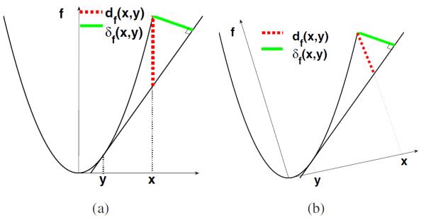
d_f(x, y) (dotted line) is BD, δ_f(x, y) (bold line) is TBD, and the two arrows indicate the coordinate system. (a) d_f(x, y) and δ_f(x, y) before rotating the coordinate system. (b) d_f(x, y) and δ_f(x, y) after rotating the coordinate system.

Bregman divergence has been widely used in clustering, where cluster centers are defined using the divergence. In this paper, we will define a cluster center using the TBD in conjunction with the l₁-norm that we dub as the t-center. The t-center can be viewed as the cluster representative that minimizes the l₁-norm TBD between itself and the members of a given population. We derive an analytic expression for the t-center which affords it an advantage over its rivals (for example, the χ²¹ distance based median of a population of densities). The key property of the t-center is that it is a weighted mean and the weight is inversely proportional to the magnitude of the gradient of the convex function used in defining the divergence. And since noisy data and outliers have greater gradient magnitude their influence is underplayed. In other words, t-center puts more weight on the normal data and less weight on the “extraordinary” data. In this sense, t-center is a robust and stable representative and this property makes the t-center attractive in many applications. Another salient feature of the t-center is that it can be computed very efficiently due to its analytic form and this leads to efficient clustering.

The rest of this paper is organized as follows. In Section 2 we review the conventional Bregman divergence, followed by the definition of TBD and derivation of its properties. Section 3 introduces the t-center, which is derived from TBD, and delves into its better accuracy as a representative than centers obtained from other divergence measures. Section 4 describes the shape retrieval application of TBD and the t-center. The detailed description of the experimental design and results with quantitative comparison with other divergences are presented in Section 5. Finally, we draw conclusions in Section 6.

2. Total Bregman Divergence

We first recall the definition of conventional Bregman divergence [2] and then define the TBD. Both divergences are dependent on the corresponding convex and differentiable function f : $X\to \mathbb{R}$ that induces the divergences.

2.1. Definition of TBD and Examples

Definition 2.1

[2] The Bregman divergence d associated with a real valued strictly convex and differentiable function f defined on a convex set X between points x, y ∈ X is given by,

$$d_f(x,y)=f\left(x\right)-f\left(y\right)-\langle x-y,\nabla f\left(y\right)\rangle ,$$ (1)

where ▿f(y) is the gradient of f at y and ⟨·, ·⟩, is the inner product determined by the space on which the inner product is being taken.

d_f(·, y) can be seen as the distance between the first order Taylor approximation to f at y and the function evaluated at x.

Definition 2.2

The total Bregman divergence (TBD) δ associated with a real valued strictly convex and differentiable function f defined on a convex set X between points x, y ∈ X is defined as,

$${\delta }_f(x,y)=\frac{f\left(x\right)-f\left(y\right)-\langle x-y,\nabla f\left(y\right)\rangle }{\sqrt{1+{\Vert \nabla f\left(y\right)\Vert }^2}},$$ (2)

⟨·, ·⟩ is the inner product as in definition 2.1, and ∥▿f(y)∥² = ⟨▿f(y), ▿f(y)⟩ generally.

As shown in Figure 1, d_f(·, y) measures the ordinate distance, and δ_f(·, y) measures the orthogonal distance. δ_f(·, y) can be seen as a higher order “Taylor” approximation to f at y and the function evaluated at x. Since

$$\frac{1}{\sqrt{1+{\Vert \nabla f\left(y\right)\Vert }^2}}=1-\frac{{\Vert \nabla f\left(y\right)\Vert }^2}{2}+O\left({\Vert \nabla f\left(y\right)\Vert }^4\right)$$ (3)

then

$${\delta }_f(x,y)=d_f(x,y)-\frac{{\Vert \nabla f\left(y\right)\Vert }^2}{2}{d}_f(x,y)+O\left({\Vert \nabla f\left(y\right)\Vert }^4\right)$$ (4)

where O(·) is the Big O notation, which is usually small compared to the first term and thus one can ignore it without worrying about the accuracy of the result. Also, we can choose the higher order “Taylor” expansion if necessary.

Compared to the BD, TBD contains a weight factor (the denominator) which complicates the computations. However, this structure brings up many new and interesting properties and makes TBD an “adaptive” divergence measure in many applications. Note that, in practice, X can be an interval, the Euclidean space, a d-simplex, the space of non-singular matrices or the space of functions. For instance, in the application to shape representation, we let p and q be two pdfs, and f(p): = ∫ p log p, then δ_f(p, q) becomes what we will call the total Kullback-Leibler divergence (tKL.) Note that for tKL, we define ∥▿f(q)∥² = ∫(1 + log q)²q specifically to make it integrable. Table 1 lists some TBDs with various associated convex functions.

Table 1.

TBD δ_f corresponding to f. $\stackrel{‒}{x}=1-x,\stackrel{‒}{y}=1-y,x^{\prime }$ is the transpose of x. Δ^d is d-simplex

X	f(x)	δf (x, y)	Remark
$\mathbb{R}$	x 2	(x − y)2 (1 + 4y2)−1/2	Total square loss
[0, 1]	$x\log x+\stackrel{‒}{x}\log \stackrel{‒}{x}$	$\left(x\log \frac{x}{y}+\stackrel{‒}{x}\log \frac{\stackrel{‒}{x}}{\stackrel{‒}{y}}\right)/\sqrt{1+y{(1+\log y)}^2+\stackrel{‒}{y}{(1+\log \stackrel{‒}{y})}^2}$	Total logistic loss
${\mathbb{R}}_{+}$	−log x	$\left(\frac{x}{y}-\log \frac{x}{y}-1\right)∕\sqrt{1+y^{-2}}$	Total Itakura-Saito distance
$\mathbb{R}$	ex	$(e^x-e^y-(x-y\left)e^y\right)∕\sqrt{1+e^{2y}}$
${\mathbb{R}}^d$	${\Vert x\Vert }^2$	${\Vert x-y\Vert }^2∕\sqrt{1+4{\Vert y\Vert }^2}$	Total squared Euclidean
${\mathbb{R}}^d$	x’Ax	$\left({(x-y)}^{\prime }A\right(x-y\left)\right)∕\sqrt{1+4{\Vert \mathit{Ay}\Vert }^2}$	Total Mahalanobis distance
Δ d	${\sum }_{j=1}^d{x}_j\log x_j$	$\left({\sum }_{j=1}^d{x}_j\log \frac{x_j}{y_j}\right)/\sqrt{1+{\sum }_{j=1}^d{y}_j{(1+\log y_j)}^2}$	Total KL divergence
${\mathbb{C}}^{m\times n}$	${\Vert x\Vert }_F^2$	${\Vert x-y\Vert }_F^2∕\sqrt{1+4{\Vert y\Vert }_F^2}$	Total squared Frobenius

3. The t-center

It is common and desirable to seek a center that is “reasonably” representative and easy to compute for a set of objects with similar properties. We will use the TBD to derive l₁-norm cluster center of this population namely, the t-center, and explore its properties.

Definition 3.1

Let f : $X\to \mathbb{R}$ be a convex and differentiable function and E = {x₁, x₂, · · · , x_n} be a set of n points in X, then, the l_p-norm TBD δ^p_f between a point x ∈ X and E associated with f and l_p norm is defined as

$${\delta }_f^p(x,E)={\left(\sum _{i=1}^n{\left({\delta }_f\right(x,x_i\left)\right)}^p\right)}^{1∕p}.$$ (5)

The l_p-norm center $x_p^{\ast }$ is defined as

$$x_p^{\ast }=\arg \underset{x}{\min }{\delta }_f^p(x,E).$$ (6)

3.1. l₁-norm t-center x*

We obtain the l₁-norm t-center x* of E by solving the following minimization problem

$$x^{\ast }=\arg \underset{x}{\min }{\delta }_f^1(x,E)=\arg \underset{x}{\min }\sum _{i=1}^n{\delta }_f(x,x_i).$$ (7)

x* has advantages over other centers resulting from the norms with p > 1 in the sense that x* is the median which is stable and robust to outliers. Moreover, it has a closed form expression which makes its computationally attractive.

To find x*, we take the derivative of $F\left(x\right)={\sum }_{i=1}^n{\delta }_f(x,x_i)$ with respect to x, and set it to 0, giving,

$$\nabla F\left(x\right)=\sum _{i=1}^n\frac{\nabla f\left(x\right)-\nabla f\left(x_i\right)}{\sqrt{1+{\Vert \nabla f\left(x_i\right)\Vert }^2}}=0.$$ (8)

Solving (8) yields:

$$\nabla f\left(x^{\ast }\right)=\left(\sum _{i=1}^n{w}_i\nabla f\left(x_i\right)\right)/\left(\sum _{i=1}^n{w}_i\right),$$ (9)

where w_i = (1 + ∥▿f(x_i)∥²)^−1/2 is the weight for its corresponding ▿f(x_i). Since δ_f(·, y) is convex for any fixed y ∈ X, we know that $F\left(x\right)={\delta }_f^1(x,E)$ is also convex as it is the sum of n convex functions. Hence, the solution to (8) i.e. the t-center x*, exists and is indeed a minimizer of F(x). We summarize this result in the following theorem.

Theorem 3.1

The gradient at the l₁-norm t-center x* is a weighted Euclidean average of the gradient of all the elements in the set E = {x₁, x₂, · · · , x_n}. The weights are given by w_i = (1 + ∥▿f(x_i)∥²)^−1/2. Moreover, x* is unique.

Theorem (3.1) reveals that the t-center has a closed form expression, which is a weighted average, and the weight is inversely proportional to the magnitude of the gradient of f at the corresponding element. Also, since f is convex, ▿f is monotonic, and x* is unique. For a better illustration, we provide two concrete examples of TBD with their t-centers in explicit form.

• tSL (total square loss): f(x) = x², the t-center

  $$x^{\ast }=\left(\sum _i{w}_i{x}_i\right)/\sum _i{w}_i,w_i=\frac{1}{\sqrt{1+4x_i^2}};$$ (10)

• Exponentials: f(x) = e^x, the t-center $x^{\ast }=\left({\sum }_i{w}_i{x}_i\right)∕\left({\sum }_i{w}_i\right)$, where$w_i={(1+e^{2x_i})}^{-1∕2}$;

4. Application of TBD to shape retrieval

We propose an efficient and accurate method for shape retrieval that includes an easy to use shape representation, and an analytical shape dissimilarity divergence measure. Also, we present an efficient scheme to solve the computationally expensive problem encountered when retrieving from a large database. The scheme is composed of clustering and pruning, which will be elaborated on in section 4.3.

4.1. Shape representation

A time and space efficient shape representation is fundamental to shape retrieval. Given a segmented shape (or a binary image), we use a mixture of Gaussians [5, 9] to represent it. The procedure for obtaining the mixture of Gaussians from a shape is composed of three steps. First, we extract the 2D points on the shape boundary, since MPEG-7 shapes are binary, the points that have nonzero gradient lie on the boundary; after getting the 2D boundary points for every shape, we use the affine alignment algorithm proposed by Ho et al. [8] to align these points, e.g., given two sets of points ${\left\{x_i\right\}}_{i=1}^m$ and ${\left\{y_j\right\}}_{j=1}^n$, we can find affine alignment $(A,b),A\in \mathbf{GL}{\left(2\right)}^2,b\in {\mathbb{R}}^2$, such that g(A, b) = ∑_i min_j{(Ax_i+b−y_j)²} achieves a minimum, and then we use the aligned ${\{{\stackrel{‒}{x}}_i\mid {\stackrel{‒}{x}}_i={\mathit{Ax}}_i+b\}}_{i=1}^m$ to represent the original point set ${\left\{x_i\right\}}_{i=1}^m$; finally, we compute the mixture of Gaussians from the aligned boundary points. A parametric mixture of Gaussians is a weighted combination of Gaussian kernels, and can be written as

$$p\left(x\right)=\sum _i^m{a}_i\mathcal{N}(x;{\mu }_i,{\Sigma }_i),0\le a_i\le 1,\sum _i^m{a}_i=1,$$ (11)

$\mathcal{N}(x;{\mu }_i,{\Sigma }_i)$ is the Gaussian density with mean μ_i, variance ∑_i, and weight a_i in the mixture model. The mixture model is obtained through an application of the Expectation-Maximization (EM) algorithm and iteratively optimizing the centers and widths of the Gaussian kernels. The above process is depicted using the flow chart shown below, with some concrete examples shown in Figure 2.

Figure 2.

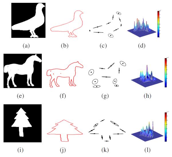
Left to right: original shapes; aligned boundaries; mixture of Gaussians with 10 components, the dot inside each circle is the mean of the corresponding Gaussian density function; 3D view of the mixture of Gaussians.

4.2. Shape dissimilarity comparison using tSL

After getting the mixture of Gaussians representation of each shape, we use tSL (total square loss divergence) to compare two mixtures of Gaussians, and take the difference as the dissimilarity between the corresponding shapes. Suppose two shapes have the following mixture of Gaussians p₁ and p₂ representation,

$$p_l\left(x\right)=\sum _i^m{a}_i^{\left(l\right)}\mathcal{N}(x;{\mu }_i^{\left(l\right)},{\Sigma }_i^{\left(l\right)}),l=1,2,$$ (12)

Since

$$\int \mathcal{N}(x;{\mu }_1,{\Sigma }_1)\mathcal{N}(x;{\mu }_2,{\Sigma }_2)=\mathcal{N}(0;{\mu }_1-{\mu }_2,{\Sigma }_1+{\Sigma }_2),$$ (13)

$$\mathit{tSL}(p_1,p_2)=\frac{\int {(p_1-p_2)}^2\mathit{dx}}{\sqrt{1+\int 4p_2^2\mathit{dx}}}=\frac{d_1+d_2-d_{1,2}}{\sqrt{1+4d_2}},$$ (14)

where

$$\begin{array}{cc}\hfill d_l& =\sum _{i,j=1}^m{a}_i^{\left(l\right)}{a}_j^{\left(l\right)}\mathcal{N}(0;{\mu }_i^{\left(l\right)}-{\mu }_j^{\left(l\right)},{\Sigma }_i^{\left(l\right)}+{\Sigma }_j^{\left(l\right)});l=1,2\hfill \\ \hfill d_{1,2}& =2\sum _{i,j=1}^m{a}_i^{\left(1\right)}{a}_j^{\left(2\right)}\mathcal{N}(0;{\mu }_i^{\left(1\right)}-{\mu }_j^{\left(2\right)},{\Sigma }_i^{\left(1\right)}+{\Sigma }_j^{\left(2\right)}).\hfill \end{array}$$

Given a set of mixture of Gaussians ${\left\{p_l\right\}}_{l=1}^n$, their t-center can be obtained from equation (10), which is

$$p^{\ast }=\frac{\sum _{l=1}^n{w}_l{p}_l}{\sum _{l=1}^n{w}_l},w_l={(1+4d_l)}^{-1∕2}.$$ (15)

We evaluate the dissimilarity between the mixture of Gaussians of the query shape and the mixture of Gaussians of the shapes in the database using tSL, and the smallest dissimilarity corresponds to the best matches.

4.3. Shape retrieval in a large database

When retrieving from a small database, it is possible to apply the brute-force search method by comparing the query shape with each shape in the database one by one, however, when retrieving in a large database, it becomes extremely slow to use this brute-force search method. Therefore, we turn to a far more efficient strategy, namely divide and conquer. First, we split the whole database into small clusters and then choose a representative for each cluster. When retrieving, we only need to compare the query with each cluster’s representative, if the divergence is larger than some threshold, we will prune this whole cluster. Once the representative that best matches the query is obtained, we will recursively split the corresponding cluster into smaller clusters, and repeat the aforementioned process on each smaller cluster, and in this way, successfully seeking out the best matches. More conveniently, the step of splitting can be done offline, which saves a lot of computation time. To partition the database into smaller clusters efficiently and accurately, we utilize an idea similar to that of k-Tree [12], by dividing the database into k clusters, calculating the t-center and repeat the above process on the resulting clusters to get k sub-clusters, and accordingly get a hierarchy of clusters. The t-centers for the hierarchical clusters form the k-Tree, as shown in Figure 3

Figure 3.

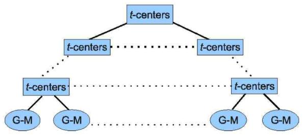
k-Tree diagram. G-M: mixture of Gaussians. Every key is a mixture of Gaussians. Each key in the inner nodes is the t-center of all keys in its children nodes. The key of a leaf is a mixture of Gaussians corresponding to an individual shape.

We should note that to maintain the accuracy, the division should follow a coarse to fine strategy (as in our experiment in 5.2), rather than fixing k, which still assures logarithmic O(log n) time expense of retrieving while enhancing accuracy.

5. Experimental Results

The proposed divergence is evaluated on shape retrieval using the MPEG-7 database [10], which consists of 70 objects with 20 shapes per object. This is a fairly difficult database to perform shape retrieval because of its large intraclass variability, and, for many classes, small interclass dissimilarity. We did two groups of experiments using this database. One is retrieving in the subsets of the MPEG-7 database, each subset containing two difficult to distinguish categories of shapes. The other one is retrieving from the whole database.

5.1. Retrieval from the subsets of the MPEG-7 database

We mix two categories having similar shapes as shown in Figure 4. There are 9 groups of mixed categories, each containing the category of the top row and the category of the corresponding bottom row. We first get the mixture of Gaussians (with 10 kernels) for each shape, then set one shape as the query and compare its mixture of Gaussians with those of all other shapes using tSL, and select the shapes according to the rank of the similarity to the query.

Figure 4.

There are 9 groups of mixed categories, each of which contains the category of the top row and the category of the corresponding bottom row. Each shape in the top row is used as a query, the goal is to retrieve shapes matching the query.

The first experiment is about retrieval in a set containing the bird and the chicken categories of the MPEG-7 database, including 20 bird and 20 chicken shapes, which have various scales, orientations as well as poses. Let one bird shape be the query, remove it from the set, and the goal is to find 19 best matches to the query. Figure 5 shows the retrieval results using SL 5(a) and tSL 5(b). The top left shape in each figure is the query and the other 19 shapes are the retrieval results shown from left to right, top to bottom, ranked according to the similarity to the query. Figure 5 illustrates that tSL can retrieve all the bird shapes even though there is a large amount of variation in the scales, orientations and poses.

Figure 5.

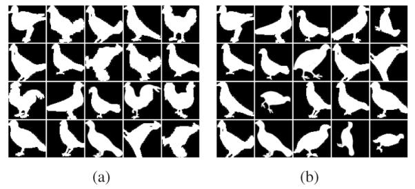
Retrieval using SL (a) and tSL (b). The top left shape in each figure is the query. The other shapes are retrieval results, shown from left to right, top to bottom, according to the rank of the similarity to the query.

Table 2 presents the comparison of the hit rate (the number of correctly retrieved shapes divided by 19) for retrieving other mixed categories in Figure 4 using SL and tSL.

Table 2.

Hit rate of shape retrieval using SL and tSL on mixture of two categories of similar shapes shown in Figure 4.

Hit rate(%)	fork	guitar	tree	deer
SL	52.63	68.42	57.89	57.89
tSL	94.74	100	94.74	84.21
Hit rate(%)	horse	cup	sea-snake	watch
SL	52.63	52.63	63.16	68.42
tSL	84.21	89.47	94.74	100

5.2. Retrieval from the entire MPEG-7 database

As described in 4.3, we first perform clustering and then do retrieval. For the clustering part, we apply a variation of k-Tree method by setting k = 10 at the first level of clustering, 7 at the second level, 5 at the third level and 2 at all following levels of clustering, so the average number of shapes in each level cluster is 140, 20, 4, 2, and 1. We compare the clustering accuracy of tSL, χ² and SL by a reasonable measure, which is the optimal number of categories per cluster divided by the average number of categories in each cluster. Figure 6 compares the clustering accuracy of tSL, χ² and SL, which shows that tSL has a high clustering accuracy, implying a strong ability to detect outliers and distinguish shapes from different categories.

Figure 6.

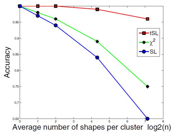
Comparison of clustering accuracy of tSL, χ² and SL, versus average number of shapes per cluster.

The evaluation of accuracy for retrieving in the whole MPEG-7 database is based on the recognition rate [6]. Table 3 lists the recognition rate obtained using various techniques, and as evident, our method outperforms all others.

Table 3.

Recognition rates comparison

Technique	Recognition rate (%)
Mixture of Gaussians + tSL	89.1
Mixture of Gaussians + χ2	63.3
Mixture of Gaussians + SL	56.7
Shape-tree[6]	87.7
IDSC + DP + EMD[14]	86.56
Hierarchical Procrustes [15]	86.35
IDSC + DP [13]	85.4
Shape L’Âne Rouge[18]	85.25
Generative Models [21]	80.03
Curve Edit [19]	78.14
SC + TPS [3] [3]	76.51
Visual Parts [10]	76.45
CSS [16]	75.44

6. Conclusions

We presented a new dissimilarity measure dubbed the total Bregman divergence(TBD), and its l₁-norm based center namely, the t-center, which has an analytic form, is stable and robust to noise and outliers. We demonstrated the salient features of TBD and the t-center using an accessible shape retrieval scheme. The results show that the t-center is a good representative of the clusters and that TBD has superior performance compared to competing methods in literature.

References

- [1].Amari S. Differential-Geometrical Methods in Statistics. Springer Berlin Heidelberg. 1985 [Google Scholar]
- [2].Banerjee A, Merugu S, Dhillon IS, Ghosh J. Clustering with Bregman divergences. J. Mach. Learn. Res. 2005;6:1705–1749. [Google Scholar]
- [3].Belongie S, Malik J, Puzicha J. Shape matching and object recognition using shape contexts. IEEE Trans. Pattern Anal. Mach. Intell. 2002;24:509–522. [Google Scholar]
- [4].Bregman LM. The relaxation method of finding the common points of convex sets and its application to the solution of problems in convex programming. USSR Comput. Math. and Math. Phys. 1967;7:200–217. [Google Scholar]
- [5].Chui H, Rangarajan A. A feature registration framework using mixture models. IEEE Workshop on Math. Methods in Biomedical Image Anal. 2000:190–197. [Google Scholar]
- [6].Felzenszwalb P, Schwartz J. Hierarchical matching of deformable shapes. IEEE CVPR. 2007:1–8. [Google Scholar]
- [7].Frigyik BA, Srivastava S, Gupta MR. Functional Bregman divergence. Int. Symp. Inf. Theory. 2008;54 [Google Scholar]
- [8].Ho J, Yang M, Rangarajan A, Vemuri B. A new affine registration algorithm for matching 2D point sets. IEEE Workshop on Appl. of Comput. Vis. 2007;89:25–30. [Google Scholar]
- [9].Jian B, Vemuri BC. A robust algorithm for point set registration using mixture of gaussians. IEEE ICCV. 2005;2:1246–1251. doi: 10.1109/ICCV.2005.17. [DOI] [PMC free article] [PubMed] [Google Scholar]
- [10].Latecki LJ, Lakamper R, Eckhardt U. Shape descriptors for non-rigid shapes with a single closed contour. IEEE CVPR. 2000;1:424–429. [Google Scholar]
- [11].Kullback S. Information Theory and Statistics. Wiley; New York: 1959. [Google Scholar]
- [12].Lancaster J, et al. k-Tree method for high-speed spatial normalization. Human Brain Mapping. 1998;6:358–363. doi: 10.1002/(SICI)1097-0193(1998)6:5/6<358::AID-HBM5>3.0.CO;2-L. [DOI] [PMC free article] [PubMed] [Google Scholar]
- [13].Ling H, Jacobs D. Using the inner-distance for classification of articulated shapes. IEEE CVPR. 2005;2 [Google Scholar]
- [14].Ling H, Okada K. An efficient earth movers distance algorithm for robust histogram comparison. IEEE Trans. Pattern Anal. Mach. Intell. 2007;29:840–853. doi: 10.1109/TPAMI.2007.1058. [DOI] [PubMed] [Google Scholar]
- [15].McNeill G, Vijayakumar S. Hierarchical procrustes matching for shape retrieval. IEEE CVPR. 2006;1 [Google Scholar]
- [16].Mokhtarian F, Abbasi S, Kittler J. Efficient and robust retrieval by shape content through curvature scale space. Int. Workshop on Image Databases and Multi-Media Search. 1997:51–58. [Google Scholar]
- [17].Nielsen F, Nock R. On the smallest enclosing information disk. Inf. Process. Lett. 2008;105:93–97. [Google Scholar]
- [18].Peter A, Rangarajan A, Ho J. Shape L’Ane rouge: Sliding wavelets for indexing and retrieval. IEEE CVPR. 2008 doi: 10.1109/CVPR.2008.4587838. [DOI] [PMC free article] [PubMed] [Google Scholar]
- [19].Sebastian T, Klein P, Kimia B. On aligning curves. IEEE PAMI. 2003:116–125. [Google Scholar]
- [20].Srivastava A, Jermyn I, Joshi S. Riemannian analysis of probability density functions with applications in vision. IEEE CVPR. 2007:1–8. [Google Scholar]
- [21].Tu Z, Yuille A. Shape matching and recognition: Using generative models and informative features. ECCV. 2004;3:195–209. [Google Scholar]
- [22].Zhang J. Divergence function, duality, and convex analysis. Neural Computation. 2004;16:159–195. doi: 10.1162/08997660460734047. [DOI] [PubMed] [Google Scholar]