Dissecting cancer heterogeneity with a probabilistic genotype-phenotype model

Abstract

One of the obstacles hindering a better understanding of cancer is its heterogeneity. However, computational approaches to model cancer heterogeneity have lagged behind. To bridge this gap, we have developed a new probabilistic approach that models individual cancer cases as mixtures of subtypes. Our approach can be seen as a meta-model that summarizes the results of a large number of alternative models. It does not assume predefined subtypes nor does it assume that such subtypes have to be sharply defined. Instead given a measure of phenotypic similarity between patients and a list of potential explanatory features, such as mutations, copy number variation, microRNA levels, etc., it explains phenotypic similarities with the help of these features. We applied our approach to Glioblastoma Multiforme (GBM). The resulting model Prob_GBM, not only correctly inferred known relationships but also identified new properties underlining phenotypic similarities. The proposed probabilistic framework can be applied to model relations between similarity of gene expression and a broad spectrum of potential genetic causes.

INTRODUCTION

Uncovering genetic causes of complex diseases is one of the most challenging open questions in systems biology research. Complex diseases are typically heterogeneous. This disease heterogeneity can be observed on many levels: (i) organismal level phenotype such as survival time, (ii) molecular level phenotype such as gene expression and (iii) underlying causes such as mutations, gene copy number variations (CNVs) or perturbations in microRNA expression level. This intricate phenotypic and genotypic landscape makes it challenging to connect phenotypes to their genotypic causes.

In the past decade systems biology emerged as a key approach to connect phenotypes to their causes (1–13). However, in the case of cancer, the relation between genotype, dysregulated pathways and higher level disease phenotypes is nontrivial owing to heterogonous nature of the disease. One attempt to deal with this heterogeneity is using set cover approaches, which provide a strategy to select a representative set of disease-associated genes from a diverse set of patient cases (2,4,5). More recently, Kim et al. (14) generalized the set cover approach to module cover. While these methods help to overcome patient-to-patient variability in inferring dysregulated genes/pathways, they do not directly model disease heterogeneity. A second line of research to understanding disease heterogeneity is through disease classification. In particular, supervised classification methods seek to learn the features distinguishing two or more predefined disease categories. Pioneered by the work of Chuang et al. (15), several approaches used expression and network connectivity information for disease classification (16–18). More recently, Setty et al. (19) developed a regression-based model for a supervised classification of Glioblastoma Multiforme (GBM). Unfortunately, obtaining reliable disease categories is highly nontrivial in most cases. Bypassing this problem, unsupervised disease classification methods typically use clustering of disease cases based on physiological or molecular characteristics such as gene expression. In the case of Glioblastoma, classification attempts used gene expression (20,21) and/or microRNA expression (22) or simultaneous clustering genome-wide DNA copy number, methylation and gene expression data (23). While each of these categorizations provides a reasonable subtyping, they are not always consistent. Such lack of consistency results in part from using different data sets and different classifying features, but also in part from attempting to classify into a small number of subtypes a set of cancer cases that does not necessarily admit a sharp partition into categories. In particular, recent studies revealed heterogeneity of cancer cells even within one patient (24).

To address these challenges, building on an idea of topic model previously used for uncovering semantic structures of text networks (25), we propose a probabilistic method of modeling of cancer heterogeneity. Our approach offers important new perspectives. First, in our approach, individual cancer cases are represented as mixtures of subtypes. These subtypes are not predefined but rather uncovered as a part of model building. Importantly, we do not assume that there exists a sharp partition into subtypes. Instead subtypes are defined in a probabilistic fashion and can be ‘fuzzy’. Next, rather than simply grouping cancer cases based on similarity of features of interest as has been done before, we distinguish two classes of features: phenotype descriptors and causative features. Phenotype descriptors are used to measure similarities between disease cases, while causative features are computationally inferred so that similar phenotypes are underlined by similar causative features.

Specifically, our model is based on two components: (i) a measure of phenotypic similarity between the patients, (ii) a list of features—possible disease causes such as mutations, CNV, microRNA levels, etc. Phenotypic similarities are used to construct a phenotype similarity graph referred to as the patient phenotype similarity network. Features in the list are used as possible explanations. We use this data to build a distribution of disease subtype models where each model is defined as a specific probability distribution of the features. This probability distribution is constructed so that the neighbors in the patient phenotype network are likely to have the same subtype assignment. We stress that we do not assume that there exists ‘the’ disease subtype model but rather we consider a distribution of such models.

Our probabilistic model allows identification of genetic aberrations, which are responsible for similarities and differences in patients’ phenotypes, pinpointing dependencies among such aberrations, and emerging probabilistic subtypes. It also provides a probabilistic way of inferring the genotype–phenotype relationship.

We applied our approach to The Cancer Genome Atlas (TCGA) GBM data to obtain a probabilistic model of the disease, Prob_GBM. We used gene expression to describe disease phenotypes, consequently the patient network was built based on gene expression similarity. This helped us to compare results inferred from our model with the study of expression-based TCGA GBM subtypes (20). We show that while our model is largely consistent with the current knowledge about GBM, it also leads to new hypotheses.

To the best of our knowledge, this is the first time that a probabilistic model explaining patient similarity relation has been proposed in the context of studying of biological heterogeneity. Specifically, by building Prob_GBM we obtained an unsupervised model that explains expression similarities by similarities of mutations, CNVs and microRNA levels. Thus unlike pattern-discovery methods, such as iCLUSTER (26,27), which introduces hidden variables for subtype membership to associate genotypic variations with gene expression, our approach models the actual relation between putative genetic causes and expression phenotype. Specifically, it ensures that pairs of patients with a similar gene expression pattern (patients connected by an edge in the patient similarity graph) are underlined by similar features and that subtypes are defined as a probability distribution of these features. Because our model construction ensures that the distribution of features has explanatory power, in the case when the considered genotypic variations cannot explain expression variations the model cannot be built. There is no requirement for sufficient explanatory power of causative features in co-clustering methods.

MATERIALS AND METHODS

The general framework for the construction of the new probabilistic meta-model

The input for building the model are (i) a patient similarity network where each node corresponds to a patient and edges are defined based on phenotypic similarity between patients (here gene expression), (ii) a set of features assigned to each node (patient). The features describe genotypic alternations or perturbed regulatory elements and are selected so that similarities between these alterations explain observed (pairwise) phenotype similarities. The disease is represented by a distribution of disease subtype models, where each disease subtype is defined by a set of features and their probabilities. The outline of the method is illustrated graphically in Figure 1. In the subsequent subsections, we will explain each element of the approach in more detail.

Figure 1.

Inference of the probabilistic model of disease subtypes. (A) The input to the inference algorithm is the patient phenotype similarity network and a set of genomic factors (mutations, CNVs, etc.) (B) Each disease subtype (K = 4) is modeled by a distribution of the factors (shown as boxes). Each patient has some probability of belonging to each subtype thus genetic factors of each patient are mixtures of genetic characteristic of each subtype. (C) The links between patients are modeled as binary variables where a probability of a link is defined by the similarity of the probabilistic subtype assignment. (D) Final model where patients are colored based on the most likely subtype assignment and uncolored nodes represent defining genomic factors.

Patient network and explanatory features

The patient network represents the similarity between patients’ disease phenotypes. This network can be defined based on a diverse set of data. Specifically, we assume that patients’ attributes are of two types. One group describes patient phenotype and is used to define patient similarity network. In this study using GBM TCGA data, we regard gene expression profile as the phenotype. Consequently, in our patient network, two patients are connected when their expression patterns are similar as assessed by the Pearson correlation coefficient. Using expression data to define patient phenotypic similarity allows us to relate our probabilistic model to the expression-based classification from the GBM literature. The second group of attributes consists of features used to explain phenotypic similarities. Because we wanted to uncover genetic underpinning of phenotypic similarities, we used mutations, gene CNVs and microRNA dysregulation, all of which have been reported to affect the susceptibility of many disorders including cancers (28,29). Here, we focus on regulatory roles of microRNAs in cancer even though their expressions can also be considered as molecular-level phenotypes. When treating microRNA as phenotypes, however, we would need to have the information on their causative genomic abnormalities including copy number changes and mutations, which are generally unavailable. At the same time, it is reasonable to use microRNA expression level as a causative feature for gene expression. In summary, we associate with each patient the set of genotypic features that characterize this patient with the aim of identifying abnormalities to explain phenotypic similarities and using their distribution to define subtypes as described below.

Model formalism

In brief, we model the patient network with a probabilistic generative process. Assuming K latent disease subtypes, features are considered as observations generated by a probabilistic process composed of K subprocesses each corresponding to one of the disease subtypes. The method of selecting appropriate K used in this study is described in the results section. Each patient is assumed to belong to each of the subtypes with some probability and each subtype is defined by a probability distribution of the explanatory features. Thus the explanatory features of each patient are generated according to a distribution, which is a mixture of the distributions of all subtypes (Figure 1B). The links between patients are modeled as binary variables whose distribution is based on the similarity of the subtype memberships of the two patients (Figure 1C). This allows defining disease subtypes using features that are not used to describe disease phenotype while ensuring that patients with similar disease phenotype will have similar subtype assignment. Intuitively, our probabilistic model can be seen as a meta-model defined by combining 1000 models.

More formally, P patients are profiled with a set of N underlying features (genomic aberrations) where each feature is described by a discrete value (microRNA expression is also represented by integers as described in methods). We describe the ith aberration in pth patient as a discrete random variable g_p,i.. Patient network is described by P² binary random variables l_p,p′ where l_p,p′ is set to 1 if there is a link between patients p and p′. Each disease subtype β_k is defined as a distribution over the genomic aberrations. This observed patient network is assumed to be generated by the following hierarchical sampling process. First, for each patient p, draw subtype proportions θ_p from the K-dimensional Dirichlet distribution. For each genomic factor g_p,i, draw the latent subtype assignment z_p,i from the multinomial distribution defined by θ_p and randomly choose a genomic factor from the corresponding multinomial distribution. Finally, for each pair of patients (p, p′) draw the binary link variable l_p,p′ from the distribution defined by the link probability function ψ. This function is exponentially dependent on the inner product of two vectors of subtype assignments z_p and z_p′ that generated their genomic aberrations. This means that the specific subtypes used to generate the genomic aberrations are those used to generate the links.

From this generative process, the latent variable Θ = {θ_p} associates patients with subtypes and Z = {z_p,i} determines the probability of links in the patient similarity graph and the subtype assignments of features, which are distributed according to B = {β_k}. By estimating Θ, B and Z, we obtain the probability with which each patient belongs to each subtype, the distribution of genomic aberrations defining each subtype, and probability with which each two patients are linked in the patient network.

Inference of the model

The generative process presented in the previous section corresponds to the following joint distribution of observed and latent variables:

Now, our goal turns to the computational problem, that is, to calculate the following posterior distribution of the latent variables Θ, Z and B conditioned on the observed patient network represented by G and L:

Here, p(G,L), the marginal probability of observations, is a major obstacle to achieving our goal. Theoretically, this can be obtained by marginalizing out the latent variables, namely, summing the joint distribution over every possible instantiation of the latent variables. In practice, however, it is often computationally intractable because the number of possible cases is innumerable. Many researchers in various fields have tried to come up with new algorithms for more accurate and more efficient approximation of this probability. In this study, we adopt the collapsed Gibbs sampling algorithm (http://cran.r-project.org/web/packages/lda/) for relational topic models that has been successfully applied to processing document network data (25) as described below.

Estimation of the model

Each feature in the patient data sets is considered in turn, and the probability of assigning each feature into each subtype is estimated conditioned on the subtype assignments to all other features. This conditional distribution can be represented as follows:

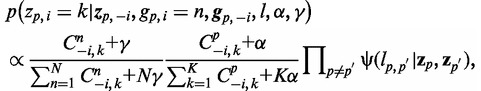where represnts all other assignment excluding the current assignment, α and γ are the Dirichlet hyperparameters for subtype proportions and feature multinomial distributions, respectively. denotes the number of times feature n is assigned to subtype k excluding the current assignment, and denotes the number of times subtype k is assigned to some features in a patient excluding the current assignment. An exponential link probability function is applied so that rapidly approaches 1 when the inner product of two vectors of subtype assignments z_p and z_p′ is large. Here, it should be noted that Θ (association of patients with subtypes) and B (distribution of features) are integrated out when sampling of subtype assignments is performed. Such a collapsed Gibbs sampling starts with random assignments of subtype, thus the samples from the early stages of the process may inaccurately represent the posterior distribution. In practice, however, it has been shown to work well and can speed up the convergence of standard (noncollapsed) Gibbs sampling over Θ, B and Z.

By the above sampling algorithm, we obtained the number of times features in each patient were assigned to each subtype. This means that we can estimate the empirical subtype distributions per patient as follows:

Supplementary Figures S4A–E illustrate these probabilities for each patient in our GBM dataset when we set K = 4. The sampling algorithm also provides the number of times a feature was assigned to a subtype. From this number, we can similarly estimate the probability of each feature n under subtype k as follows:

Because the ordering of subtypes is exchangeable between runs of the algorithm, subtype k in one run might be different from subtype k in another run. Thus, we assess the stability of algorithm by considering how many times a pair of patients (or features) and patient–feature pairs have the same subtype assignments in multiple runs. For each run of algorithm, we check if is equal to (or is equal to ) and . How often these statements are true for 1000 runs of algorithms, that is, patient–patient (or feature–feature) and patient–feature association probabilities are illustrated in Figures 2B and 3. In every run, both α and γ are set to 0.1, respectively.

Figure 2.

(A) Patient network based on expression correlation. Colors correspond to gene expression-based subtypes identified by Verhaak et al. where red denotes the Mesenchymal TCGA subtype, blue Classical, purple Proneural and green Neural. The numbers denote the patient groups from panel B. Note that the Mesenchymal and Proneural subtypes are highly connected, the Classical subtype is somewhat less connected, while the Neural is not well separated from the Proneural subtype. (B) Patient–patient heat map illustrating frequencies with which each pair of patients has the same subtype assignment over all 1000 models in our meta-model. (C) TCGA subtype assignment based on gene expression. (D) Probabilistic subtype assignment over 1000 models (see text).

Figure 3.

Integrated result from 1000 subtype models for feature–feature and feature–patient relations. The two heat maps illustrate frequencies with which each feature–feature (A) patient–feature (B) pair has the same subtype assignment according to the empirical distribution (see ‘Materials and Methods’ section). Supplementary materials online allow exploring the heat map in an interactive way zooming in on individual features).

The quality of the results can be affected by the selection of number of subtypes. Too few subtypes would hinder detection of more subtle differences and too many might lead to noisy and uninterpretable patient groups. One way to address this challenge is to consider various alternatives and then choose the number leading to the best clustering stability as in Brunet et al. (30). While it could be a tedious and time-consuming procedure especially for large data sets, it allows us to select the appropriate number of subtypes for the given dataset based on a quantitative measure rather than a subjective evaluation. By using patient–patient association probability as a measure of similarity, an average linkage hierarchical cluster tree is generated (the order of samples in the heat map is also derived by this tree). Then, cophenetic correlation coefficients for different K are calculated to evaluate the quality of alternative solutions. If the pairwise associations vary little run by run, most association probabilities are close to 0 or 1. In this case, the cophenetic correlation coefficient is also close to 1 because it is a measure of how well the tree represents the association probability. The results of this procedure for the basic and extended sets are illustrated in Supplementary Figures S2 and S3, respectively. Here, we selected K = 4, which has the largest cophenetic correlation for the basic set. We note that despite the difference in the value of K, the patient–patient heat map did not change significantly.

Data

To construct the patient network, we use a unified gene expression profile obtained by applying factor analysis to genes present on three different microarray platforms (31). After assigning unified expression measures to genes present on all three platforms, rescaling unified measures and filtering out unreliable or uninformative genes, final unified gene expression estimates of 1740 genes for every patient are acquired (https://tcga-data.nci.nih.gov/docs/publications/gbm_exp/). As a distance metric, one minus the correlation between patients is calculated. Copy number data from several high-throughput technologies were analyzed using three different computational methods and reported as gene-specific amplification and deletion calls (32). For more accurate analysis, we adopt consensus calls, which are supported by at least two independent platforms and two independent methods. (For five patients that do not have consensus copy number calls, we obtained the calls from just one platform and one method.) Each random variable of copy number genomic factors is set to 1 for single-copy amplification or hemizygous deletion and to 2 for multiple-copy amplification or homozygous deletion. (See the supplementary information of (32) for the implementation of these methods.) Consensus calls are downloaded from the cBio Cancer Genomic Portal (33) and 218 variables for copy number amplification and deletion are finally considered in our analysis. Through the same portal, we acquired mutation profiles generated by exon sequencing. Although these profiles include different mutation types such as single nucleotide mutation, insertion and deletion, we treat them equally. Thus, we considered 418 variables for genes that have a mutation in at least one patient and set their values to 2 when the corresponding genes are mutated in a particular patient. One hundred twenty-one highly variable, survival-related or neurodevelopmental-related microRNAs are also selected (22) and their expression profiles (http://compbio.med.harvard.edu/Supplements/CancerRes11.html) are standardized by subtracting the mean expression and dividing the difference by standard deviation. Similar to random variables for copy number alterations, two random variables per microRNA are considered and they indicate how many standard deviations away above or below each mean microRNA expression are, respectively. That is, we set this variable to 2 if the expression is >2 standard deviations from the mean and set to 1 if the expression is between 1 and 2 standard deviations.

RESULTS AND DISCUSSION

Prob_GBM meta-model

First, we present the results of applying our probabilistic modeling to GBM data, which has 202 patients represented in TCGA. This is an ideal data set for our purpose because GBM has been shown to be heterogeneous and the TCGA data set has been previously used for disease classification and identification for subtype-specific genetic abnormalities. The technical details of data processing are described in the ‘Materials and Methods’ section.

To construct the patient network, we use the unified gene expression profile obtained by applying factor analysis to genes present on three different microarray platforms (31) (see ‘Materials and Methods’ section). Using (1 - expression_correlation) as the distance measure, we selected the top 5% of the closest pairs as network edges. We considered also 3 and 10% cutoffs but the first produced sparse network, which would miss many patient similarities, while at the 10% cutoff, we observed an increased number of edges between different subgroups without a significant increase of connectivity within sparsely connected blue and green clusters (Figure 2). Finally, we confirmed that the top 5% cutoff provides reasonable modularity of the patient network by graphing the distribution of node clustering coefficients and overall network clustering coefficient at various cutoffs (Supplementary Figure S1). The resulting network is presented in Figure 2A, where nodes are colored based on their classification into four expression-based TCGA groups (31).

As the explanatory features associated with nodes (patients), we consider copy number alternations, mutations and microRNA expression. Specifically, the model has one random variable per each gene and per each type of a genetic variation observed in this gene. We treat amplification and deletion as two different types of variations. A random variable corresponding to the deletion is set to 1 for hemizygous deletion and to 2 for homozygous deletion. An application variable is set to 1 for single-copy and 2 for multiple-copy amplification (see ‘Materials and Methods’ section). There is one variable per gene to represent mutation. Note that it is possible to set a separate variable for each specific mutation in each gene, but to simplify the model we just use one variable to represent the presence or the absence of a mutation. Finally, we consider two sets of the over- or under-expression of microRNAs. The first is the set of the 121 highly variable, survival-related or neurodevelopmental-related microRNAs identified in (22) and the second has all remaining 470 microRNAs after removing only viral origin microRNAs (22). We refer to the set of features that include mutation, CNV and small microRNA set as ‘basic’ and mutation, CNV and large microRNA set as ‘extended’. We consider over- and under-expression as two different types of alterations and thus they are represented by two groups of random variables. In either case, each variable indicates if the expression is >1 or 2 standard deviations from the mean microRNA expression are (see ‘Materials and Methods’ section).

Finally, we evaluated the stability of the learning algorithm for the model with different K (K = 3, 4, 5 and 6 were tested in this article, see ‘Materials and Methods’ section). This parameter setting allowed us to examine the consistency of our model with the knowledge gained by TCGA classification and to demonstrate its increased explanatory power relative to this standard (see ‘Materials and Methods’ section). We selected K = 4 for the basic set and K = 5 for the extended set (Supplementary Figures S2 and S3). Importantly for all K, there was one subgroup that contained a singleton outlier. This outlier was a patient with unusual number of mutation and atypical expression pattern. We ignore this outlier in the discussions below.

Relation of probabilistic subtypes in Prob_GBM meta-model and expression based TCGA subtypes

Recall that the Prob_GBM meta-model is defined by 1000 subtype models. In each such model, the subtypes might be defined by a different distribution of features and the assignment of the patients to subtypes is probabilistic. As an illustration, we zoom in on one such subtype model in Supplementary Figure S4. To obtain the Prob_GBM meta-model, we integrated 1000 instances of subtype models. Note that while the models might have a different distribution of defining features, they are all optimized to explain the same patient phenotype similarity network drawing the explanations from the same explanatory features. Thus, these models are not unrelated and the distribution of their recurrent features provides a link between explanatory features and phenotypic properties. One way to summarize the final meta-model is to display, for all pairs of patients, the frequency of being categorized into the same subtype (see ‘Materials and Methods’ section). The heat map representing these frequencies is shown in Figure 2B. The colored bar below the heat map (Figure 2C) shows the assignment of the corresponding patient to the TCGA group in (31). From this figure we can see that there are three core groups of patients, generally consistent with the TCGA annotation as Mesenchymal, Classical and Proneural, which with probability close to one belong to the same subtype in each model. We can also summarize the subtype assignment over the 1000 models of the Prob_GBM meta-model. Specifically, for all subtypes models, we can label the three subtypes as Mesenchymal, Classical, Proneural and ‘neither’ based on the probability of co-assignment of a given patient with a fixed representative of each ‘core’ group. In this way we summarized, over all 1000 subtype models, the probability of each patient being in each of four probabilistic subtypes. These probabilities are shown in Figure 2D. Note for each of these three subtypes, there is a large group of patients where the TCGA annotation of patients agrees perfectly with the maximal probability assignment. Interestingly, the patients for which the most likely subgroup is not the same as the expression-based TCGA classification are typically best represented as mixtures of subtypes. In particular, TCGA expression-based classification also contains a controversial Neural TCGA subtype (green). This subtype is often considered to be not well defined (23,34). Our mixture model elegantly explains this discrepancy. Specifically, it reveals that the genotypic features of many patients in this group are best described as a mixture of Proneural and Mesenchymal subtypes. For example, subgroup 22 in Figures 2A and B is such a group of patients that frequently co-assigned with the core Mesenchymal group.

We were interested to see if the Neural subtype would emerge as an individual subtype when we increase the number of subtypes to K = 5 and, at the same time, use the extended features, which include the large microRNA set as explanatory features. However, the Neural subtype also did not emerge as an individual subtype in this case. The corresponding heat map is shown in Supplementary File S2. A new subtype that emerged was relatively small. It was underlined by a mutation in a protein kinase A-anchoring protein AKAP2, Matrix Metal Protease MMP15, Cadherin-1 protein and a number of microRNAs among which upregulation of miR-584 were most prominent. miR-584 has been suggested to decrease invasion ability in human clear cell renal cell carcinoma (35). These annotations strongly suggest a relation of this potential subtype to the tumor invasion process. However, a larger set of samples is needed to confirm that this group can indeed be considered a separate subtype.

Finally, to keep the findings of this section in the correct perspective, we reiterate that while we discussed the emergence of subtypes, our approach is not a clustering procedure. In our model, emergence of probabilistic subtypes is based on the explanatory ability of the selected features. Thus the fact that Neural subtype has not emerged as a separate subtype in our model does not contradict the results of (20). Instead it signifies that the expression similarities between the patients in this group are best explained by a combination of explanatory features delineating the other two groups.

Genetic causes underlying Prob_GBM probabilistic subtypes

Next, we analyzed mutations, copy number alterations and microRNA levels underlying Prob_GBM meta-model. For each of the 1,000 subtype models, we can estimate the probability that a feature underlines this subtype (see ‘Materials and Methods’ section). For any two features we can also estimate the frequency of jointly underlying the same subtype. This frequency distribution can be summarized as feature–feature heat map (Figure 3A). Similarly, we can estimate the frequency of assigning same subtype to every patient–feature and use it to construct patient–feature heat map (Figure 3B). Interactive visualization of the heat maps are enabled in Supplementary Files S1 and S2.

We started by validating the method and confirming that the Prob_GBM meta-model is consistent with known relationships. From the patient–feature heat map (Figure 3B and Supplementary File S2), we see that IDH1 mutation and PDGFRA amplification are the most prominent features underlining the group corresponding to the Proneural subtype, while NF1 mutation and deletion underlines the probabilistic subtype harboring mostly patients classified as Mesenchymal. Amplification of EGFR and deletion and mutation of PTEN are among the genetic variations underlying the subgroup corresponding to the Mesenchymal subtype but they also have a significant impact for the Classical subtype. This is in an excellent agreement with (31) and provides additional evidence that our method correctly detects genomic signals underlying gene expression similarity. In addition to the genetic factors underlying the three basic subtypes identified by Verhaak et al. (31), we confirmed the expected clinical characteristics of the groups with respect to age and necrosis (Supplementary Figure S5).

We next turned our attention to additional features that contributed to the definition of the corresponding subtypes. Because our model explains gene expression similarities, not all genetic features explaining these relations are necessarily causative for cancer. Therefore, for the purpose of the discussion below, we focused on known cancer causes and examined how these alterations contribute to the model definition. For the purpose of visualization, we extracted from the full spectrum of the relationships (Figure 3 and its interactive version in Supplementary File S2) a summary of the importance of known cancer-related genetic aberrations for defining particular subtypes. Specifically, in Figure 4, relative frequencies of oncogenic features in groups defined by the Prob_GMB meta-model are shown. For group 1 (corresponding to the Proneural subtype), in the addition to mutation in IDH1 gene and PDGFRA amplification, a significant role is played by amplifications of ERBB2 and ERBB3. There are also several additional explanatory features that underlie group 2 (corresponding to the Mesenchymal subtype). The most interesting features include deletions of cancer suppressers BRCA1, BRCA2 and deletions of FOXO1 and FOXO3. The most prominent explanatory feature for the probabilistic Classical subtype was amplification of AKT2. Interesting is also the emergence of two members of necrosis factor receptor superfamily members TNFRSF6B and TNFRSF1B. However, overall, mutations, CNVs and microRNAs used as possible features cannot completely disambiguate this subgroup as they are either not general enough (present in a small number of cases) or shared with other subtypes. This can also be appreciated in Figure 2D by observing that the members of this group belong to other two subgroups in a significant fractions of the models. As an example of the explanatory role of microRNAs, the Messemchymal group is distinguished by under-expression of miR-128, miR-137 and miR-124. It is known that miR-124 and miR-137 inhibit proliferation of GBM cells and induce differentiation of brain tumor stem cells (36), while recently miR-128 has been identified as a candidate glioma tumor suppressor for proneuronal GBM (37). In contrast, these microRNAs have relatively high expression in the Proneural probabilistic subtype.

Figure 4.

Mutations and CNV of selected cancer genes and microRNAs emerge as important for subtypes definitions. Here, color bars represent relative frequencies for groups defined by the Prob_GMB meta-model. We calculate them by considering the discretized values of each feature in the data set as a frequency. Total frequencies of the selected features over all patient samples are presented in the parenthesis.

CONCLUSIONS

While it is currently well understood that most cancers are heterogeneous, the tools to model such heterogeneities were lagging behind this understanding. In this article, we developed Prob_GBM, the first probabilistic explanatory model for cancer. Our model was constructed in an unsupervised way as a meta-model built from a large set of models that explains phenotypic similarities with the help of genetic aberration and microRNA expression. Importantly, the technique used in the construction of Prob_GBM is general and can be used to connect a differently defined phenotype similarity with a different set of putative causes.

In this article, we focused on the introduction and the validation of our approach and demonstrating its power. In the current study, we did not use methylation data as a possible explanation because it is not defined for a large subset of patients.

Because we used gene expression similarity to define phenotypic similarity between patients, if these similarities were indeed underlined by genetic and microRNA aberrations, we expected to find the corresponding drivers and, through the probabilistic model, refine the subtype definitions. Like others, we did not find support for treating the Neural TCGA as a separate subtype. Instead, our model suggests that the Neural subtype can be seen as is a mixture of the Proneural and Mesenchymal subtypes. We succeeded in identifying the features explaining the remaining subtypes. We stress that because the role of features identified by our model goes beyond simple association, if no features that explain phenotypic variability can be found, the model cannot be built.

Prob_GBM provides reach information about the relation between genetic causes and phenotypic variations allowing for identifying new relationships and postulating new hypotheses. It not only confirmed known drivers of phenotypic differences but also identified novel ones and the relationships between them. Thus, we conclude that Prob_GBM fills a significant gap between the general current understanding of cancer and existing approaches for modeling cancer diversity.

In this work, we focused on model inference and validation as well as demonstrating how the information represented in the model can be leveraged to understand disease heterogeneity in the context of relatively well-studied GBM. However, many interesting variations of the model are possible. For example, phenotype similarity might include survival time and responses to treatment. Features can be extended to include transcription factor biding, methylation, age, sex or environment. Alternatively, features can be narrowed down to microRNA only, to study the impact of these molecules alone. Our study opens the door to these and many other applications.

SUPPLEMENTARY DATA

Supplementary Data are available at NAR Online.

FUNDING

Funding for open access charge: Intramural Research Program of the National Institutes of Health, National Library of Medicine.

Conflict of interest statement. None declared.

REFERENCES

- 1.Akavia UD, Litvin O, Kim J, Sanchez-Garcia F, Kotliar D, Causton HC, Pochanard P, Mozes E, Garraway LA, Pe'er D. An integrated approach to uncover drivers of cancer. Cell. 2010;143:1005–1017. doi: 10.1016/j.cell.2010.11.013. [DOI] [PMC free article] [PubMed] [Google Scholar]
- 2.Chowdhury SA, Koyuturk M. Identification of coordinately dysregulated subnetworks in complex phenotypes. Pac. Symp. Biocomput. 2010:133–144. doi: 10.1142/9789814295291_0016. [DOI] [PubMed] [Google Scholar]
- 3.Kim YA, Przytycki JH, Wuchty S, Przytycka TM. Modeling information flow in biological networks. Phys. Biol. 2011;8:035012. doi: 10.1088/1478-3975/8/3/035012. [DOI] [PMC free article] [PubMed] [Google Scholar]
- 4.Kim YA, Wuchty S, Przytycka TM. Identifying causal genes and dysregulated pathways in complex diseases. PLoS Comput. Biol. 2011;7:e1001095. doi: 10.1371/journal.pcbi.1001095. [DOI] [PMC free article] [PubMed] [Google Scholar]
- 5.Ulitsky I, Krishnamurthy A, Karp RM, Shamir R. DEGAS: de novo discovery of dysregulated pathways in human diseases. PLoS One. 2010;5:e13367. doi: 10.1371/journal.pone.0013367. [DOI] [PMC free article] [PubMed] [Google Scholar]
- 6.Ulitsky I, Shamir R. Detecting pathways transcriptionally correlated with clinical parameters. Comput. Syst. Bioinformatics Conf. 2008;7:249–258. [PubMed] [Google Scholar]
- 7.Vandin F, Upfal E, Raphael BJ. Algorithms for detecting significantly mutated pathways in cancer. J. Comput. Biol. 2011;18:507–522. doi: 10.1089/cmb.2010.0265. [DOI] [PubMed] [Google Scholar]
- 8.Vanunu O, Magger O, Ruppin E, Shlomi T, Sharan R. Associating genes and protein complexes with disease via network propagation. PLoS Comput. Biol. 2010;6:e1000641. doi: 10.1371/journal.pcbi.1000641. [DOI] [PMC free article] [PubMed] [Google Scholar]
- 9.Yeger-Lotem E, Riva L, Su LJ, Gitler AD, Cashikar AG, King OD, Auluck PK, Geddie ML, Valastyan JS, Karger DR, et al. Bridging high-throughput genetic and transcriptional data reveals cellular responses to alpha-synuclein toxicity. Nat. Genet. 2009;41:316–323. doi: 10.1038/ng.337. [DOI] [PMC free article] [PubMed] [Google Scholar]
- 10.Tuncbag N, Braunstein A, Pagnani A, Huang SSC, Chayes J, Borgs C, Zecchina R, Fraenkel E. RECOMB. 2012:pp. 127–147. [Google Scholar]
- 11.Schadt EE, Lamb J, Yang X, Zhu J, Edwards S, Guhathakurta D, Sieberts SK, Monks S, Reitman M, Zhang C, et al. An integrative genomics approach to infer causal associations between gene expression and disease. Nat. Genet. 2005;37:710–717. doi: 10.1038/ng1589. [DOI] [PMC free article] [PubMed] [Google Scholar]
- 12.Segal E, Shapira M, Regev A, Pe'er D, Botstein D, Koller D, Friedman N. Module networks: identifying regulatory modules and their condition-specific regulators from gene expression data. Nat. Genet. 2003;34:166–176. doi: 10.1038/ng1165. [DOI] [PubMed] [Google Scholar]
- 13.Suthram S, Dudley JT, Chiang AP, Chen R, Hastie TJ, Butte AJ. Network-based elucidation of human disease similarities reveals common functional modules enriched for pluripotent drug targets. PLoS Comput. Biol. 2010;6:e1000662. doi: 10.1371/journal.pcbi.1000662. [DOI] [PMC free article] [PubMed] [Google Scholar]
- 14.Kim Y, Salari R, Wuchty S, Przytycka TM. Pacific Symposium on Biocomputing. 2013 [PMC free article] [PubMed] [Google Scholar]
- 15.Chuang HY, Lee E, Liu YT, Lee D, Ideker T. Network-based classification of breast cancer metastasis. Mol. Syst. Biol. 2007;3:140. doi: 10.1038/msb4100180. [DOI] [PMC free article] [PubMed] [Google Scholar]
- 16.Lee E, Chuang HY, Kim JW, Ideker T, Lee D. Inferring pathway activity toward precise disease classification. PLoS Comput. Biol. 2008;4:e1000217. doi: 10.1371/journal.pcbi.1000217. [DOI] [PMC free article] [PubMed] [Google Scholar]
- 17.Dao P, Colak R, Salari R, Moser F, Davicioni E, Schonhuth A, Ester M. Inferring cancer subnetwork markers using density-constrained biclustering. Bioinformatics. 2010;26:i625–i631. doi: 10.1093/bioinformatics/btq393. [DOI] [PMC free article] [PubMed] [Google Scholar]
- 18.Dao P, Wang K, Collins C, Ester M, Lapuk A, Sahinalp SC. Optimally discriminative subnetwork markers predict response to chemotherapy. Bioinformatics. 2011;27:i205–i213. doi: 10.1093/bioinformatics/btr245. [DOI] [PMC free article] [PubMed] [Google Scholar]
- 19.Setty M, Helmy K, Khan AA, Silber J, Arvey A, Neezen F, Agius P, Huse JT, Holland EC, Leslie CS. Inferring transcriptional and microRNA-mediated regulatory programs in glioblastoma. Mol. Syst. Biol. 2012;8:605. doi: 10.1038/msb.2012.37. [DOI] [PMC free article] [PubMed] [Google Scholar]
- 20.Sanai N. Integrated genomic analysis identifies clinically relevant subtypes of glioblastoma. World Neurosurg. 2010;74:4–5. doi: 10.1016/j.wneu.2010.08.011. [DOI] [PubMed] [Google Scholar]
- 21.Li A, Walling J, Ahn S, Kotliarov Y, Su Q, Quezado M, Oberholtzer JC, Park J, Zenklusen JC, Fine HA. Unsupervised analysis of transcriptomic profiles reveals six glioma subtypes. Cancer Res. 2009;69:2091–2099. doi: 10.1158/0008-5472.CAN-08-2100. [DOI] [PMC free article] [PubMed] [Google Scholar]
- 22.Kim TM, Huang W, Park R, Park PJ, Johnson MD. A developmental taxonomy of glioblastoma defined and maintained by MicroRNAs. Cancer Res. 2011;71:3387–3399. doi: 10.1158/0008-5472.CAN-10-4117. [DOI] [PMC free article] [PubMed] [Google Scholar]
- 23.Shen R, Mo Q, Schultz N, Seshan VE, Olshen AB, Huse J, Ladanyi M, Sander C. Integrative subtype discovery in glioblastoma using iCluster. PLoS One. 2012;7:e35236. doi: 10.1371/journal.pone.0035236. [DOI] [PMC free article] [PubMed] [Google Scholar]
- 24.Dalerba P, Kalisky T, Sahoo D, Rajendran PS, Rothenberg ME, Leyrat AA, Sim S, Okamoto J, Johnston DM, Qian D, et al. Single-cell dissection of transcriptional heterogeneity in human colon tumors. Nat. Biotechnol. 2011;29:1120–1127. doi: 10.1038/nbt.2038. [DOI] [PMC free article] [PubMed] [Google Scholar]
- 25.Chang J, Blei DM. Hierarchical relational models for document networks. Ann. Appl. Stat. 2010;4:124–150. [Google Scholar]
- 26.Shen R, Olshen AB, Ladanyi M. Integrative clustering of multiple genomic data types using a joint latent variable model with application to breast and lung cancer subtype analysis. Bioinformatics. 2009;25:2906–2912. doi: 10.1093/bioinformatics/btp543. [DOI] [PMC free article] [PubMed] [Google Scholar]
- 27.Mo Q, Wang S, Seshan VE, Olshen AB, Schultz N, Sander C, Powers RS, Ladanyi M, Shen R. Pattern discovery and cancer gene identification in integrated cancer genomic data. Proc. Natl Acad. Sci. USA. 2013;110:4245–4250. doi: 10.1073/pnas.1208949110. [DOI] [PMC free article] [PubMed] [Google Scholar]
- 28.Almal SH, Padh H. Implications of gene copy-number variation in health and diseases. J. Hum. Genet. 2012;57:6–13. doi: 10.1038/jhg.2011.108. [DOI] [PubMed] [Google Scholar]
- 29.Farazi TA, Spitzer JI, Morozov P, Tuschl T. miRNAs in human cancer. J. Pathol. 2011;223:102–115. doi: 10.1002/path.2806. [DOI] [PMC free article] [PubMed] [Google Scholar]
- 30.Brunet JP, Tamayo P, Golub TR, Mesirov JP. Metagenes and molecular pattern discovery using matrix factorization. Proc. Natl Acad. Sci. USA. 2004;101: 4164–4169. doi: 10.1073/pnas.0308531101. [DOI] [PMC free article] [PubMed] [Google Scholar]
- 31.Verhaak RGW, Hoadley KA, Purdom E, Wang V, Qi Y, Wilkerson MD, Miller CR, Ding L, Golub T, Mesirov JP, et al. Integrated genomic analysis identifies clinically relevant subtypes of glioblastoma characterized by abnormalities in PDGFRA, IDH1, EGFR, and NF1. Cancer Cell. 2010;17:98–110. doi: 10.1016/j.ccr.2009.12.020. [DOI] [PMC free article] [PubMed] [Google Scholar]
- 32.Chin L, Meyerson M, Aldape K, Bigner D, Mikkelsen T, VandenBerg S, Kahn A, Penny R, Ferguson ML, Gerhard DS, et al. Comprehensive genomic characterization defines human glioblastoma genes and core pathways. Nature. 2008;455:1061–1068. doi: 10.1038/nature07385. [DOI] [PMC free article] [PubMed] [Google Scholar]
- 33.Cerami E, Gao J, Dogrusoz U, Gross BE, Sumer SO, Aksoy BA, Jacobsen A, Byrne CJ, Heuer ML, Larsson E, et al. The cBio cancer genomics portal: an open platform for exploring multidimensional cancer genomics data. Cancer Discov. 2012;2:401–404. doi: 10.1158/2159-8290.CD-12-0095. [DOI] [PMC free article] [PubMed] [Google Scholar]
- 34.Huse JT, Phillips HS, Brennan CW. Molecular subclassification of diffuse gliomas: seeing order in the chaos. Glia. 2011;59:1190–1199. doi: 10.1002/glia.21165. [DOI] [PubMed] [Google Scholar]
- 35.Ueno K, Hirata H, Shahryari V, Chen Y, Zaman MS, Singh K, Tabatabai ZL, Hinoda Y, Dahiya R. Tumour suppressor microRNA-584 directly targets oncogene Rock-1 and decreases invasion ability in human clear cell renal cell carcinoma. Br. J. Cancer. 2011;104:308–315. doi: 10.1038/sj.bjc.6606028. [DOI] [PMC free article] [PubMed] [Google Scholar]
- 36.Silber J, Lim DA, Petritsch C, Persson AI, Maunakea AK, Yu M, Vandenberg SR, Ginzinger DG, James CD, Costello JF, et al. miR-124 and miR-137 inhibit proliferation of glioblastoma multiforme cells and induce differentiation of brain tumor stem cells. BMC Med. 2008;6:14. doi: 10.1186/1741-7015-6-14. [DOI] [PMC free article] [PubMed] [Google Scholar]
- 37.Papagiannakopoulos T, Friedmann-Morvinski D, Neveu P, Dugas JC, Gill RM, Huillard E, Liu C, Zong H, Rowitch DH, Barres BA, et al. Pro-neural miR-128 is a glioma tumor suppressor that targets mitogenic kinases. Oncogene. 2012;31:1884–1895. doi: 10.1038/onc.2011.380. [DOI] [PMC free article] [PubMed] [Google Scholar]
Associated Data
This section collects any data citations, data availability statements, or supplementary materials included in this article.