Bayesian Hierarchical Poisson Regression Models: An Application to a Driving Study with Kinematic Events

Abstract

Although there is evidence that teenagers are at a high risk of crashes in the early months after licensure, the driving behavior of these teenagers is not well understood. The Naturalistic Teenage Driving Study (NTDS) is the first U.S. study to document continuous driving performance of newly-licensed teenagers during their first 18 months of licensure. Counts of kinematic events such as the number of rapid accelerations are available for each trip, and their incidence rates represent different aspects of driving behavior. We propose a hierarchical Poisson regression model incorporating over-dispersion, heterogeneity, and serial correlation as well as a semiparametric mean structure. Analysis of the NTDS data is carried out with a hierarchical Bayesian framework using reversible jump Markov chain Monte Carlo algorithms to accommodate the flexible mean structure. We show that driving with a passenger and night driving decrease kinematic events, while having risky friends increases these events. Further the within-subject variation in these events is comparable to the between-subject variation. This methodology will be useful for other intensively collected longitudinal count data, where event rates are low and interest focuses on estimating the mean and variance structure of the process. This article has online supplementary materials.

Recent advances in technology for assessing gravitational force (g-force) events using accelerometers allow social scientists to carefully examine driving behavior in a naturalistic setting (100-car study; Klauer et al. 2006; Guo et al. 2010). The Naturalistic Teenage Driving Study (NTDS) is an NIH-funded undertaking that measures driving performance and risk of teenagers during their early months of licensure (Simons-Morton et al. 2011a,b). In this study, 42 newly licensed teenage drivers aged 16 to 17 from the Roanoke area in Virginia were monitored continuously during their first 18 months (between 2006 and 2009) of independent driving using in-vehicle data recording systems. The study provides valuable information on risky driving behavior, which can be assessed in terms of elevated g-force events (the term kinematic event is used interchangeably with g-force event). Counts of kinematic events are available for each trip (ignition on to ignition off), and their incidence rates represent different aspects of risky driving behavior. It is common practice in this field to derive a composite kinematic event as being the occurrence of any one of the following events at a pre-described g-force: rapid starts, hard stops, hard left turns, hard right turns, and yaw, a measure of correction after a turn (Wahlberg 2007; Simons-Morton et al. 2011a,b). Simons-Morton et al. (2012) showed in a logistic regression framework that the composite measure predicts crashes/near crashes as well as using all five measures individually. The NTDS dataset comprises more than 68,000 trips with the median of 1429.5 trips per individual (range: 157 to 3162), providing the first such intense data ever collected on teenagers. Our interest in the NTDS is on examining how the composite kinematic event rates change over time and understanding the effect of important covariates such as day or night driving, other passengers, and risky friends on these event rates. We are also interested in understanding the between- and within-individual variation in the event rates over time. The sources of variation in these longitudinal data are interesting in themselves (is the within-subject variation sizable compared to the between-subject variations?) and will be useful in designing future studies in terms of follow-up length and intensity of the measurements.

Figure 1 presents exploratory analyses for the composite kinematic events in the NTDS. Figure 1 (a) shows an overall smoothed LOWESS incidence rate, while Figure 1 (b) shows a smoothed LOWESS curve for each of the 42 participants in the study. An exploratory data analysis in Figure 1 (c) demonstrates that the intra-driver variability is large relative to the inter-driver variability. Taken together these figures demonstrate the need for incorporating a complex mean structure and both between- and within- subject variation into the modeling framework. Serial correlation may also be an issue to address in these data. Since car trips are at highly irregular time points, we use the variogram rather than the correlogram to examine the correlation structure (Diggle et al. 1994). Ideally, we would like to have a single variogram based on all possible pairs of trips driven by the same subject. This is impractical, however, because many subjects had 1-3 thousand trips, giving rise to 1-9 million pairs from just one subject. To overcome this problem, we used a subsampling approach where each trip in the original dataset is paired randomly with another trip for the same subject. This resulted in approximately 68 thousand pairs (the same size as the original dataset), for which a standard variogram could be constructed. To account for the randomness in subsampling, we repeated this procedure 10 times with the resulting variograms shown in Figure 2. The figure clearly suggests the presence of serial correlation.

Figure 1.

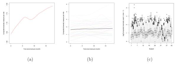
Exploratory analysis for composite kinematic events in NTDS: (a) Overall smoothed LOWESS curve of the composite kinematic event for all trips in the study; (b) Individual smoothed LOWESS curves (dotted line for each driver) compared to the overall LOWESS curve (thicker line); (c) Individual box plots for log_e(composite kinematic events/mile + 1).

Figure 2.

LOWESS smoothed empirical variograms for the composite kinematic events in the NTDS based on 10 random pairings.

The NTDS data features pose several analytic challenges. First, the model has to be flexible enough to capture the complicated mean structure, as evident from the non-linear longitudinal trajectory of the composite kinematic events in Figure 1 (a) and (b). A parametric specification of the mean structure may be too restrictive in estimating the rich pattern in these data. Second, Simons-Morton et al. (2011b) used a Poisson model with a random effect to represent between-subject variation for data analysis. However, this approach has some weaknesses since there was clear evidence for overdispersion and serial correlation. Since the appropriate modeling of the sources of variation is important for understanding the variation in risky driving over time, an important goal in this study, we need to incorporate between- and within-individual variation as well as serial correlation into the modeling framework. Third, the large number of trips at irregular intervals on each individual pose a computational challenges. In view of these challenges, we propose a Bayesian hierarchical Poisson regression model with a latent process for the long and unequally spaced sequences of count data. The latent process consists of terms for a decaying serial correlation, heterogeneity, and over-dispersion. In addition, we propose to use nonparametric regression methodology to model the longitudinal trajectory to account for time varying patterns of the outcome. To achieve an efficient Markov chain Monte Carlo (MCMC), we propose a reparametrization scheme that proves to enhance the convergence. Further, we implement a fully data-driven, adaptive knot selection scheme that identifies the optimal number and location of the knots in the longitudinal trajectory via the reversible jump MCMC (RJMCMC) algorithm (Green 5 1995; DiMatteo et al. 2001; Botts and Daniels 2008). In this paper, we use the polynomial regression spline based on truncated power basis instead of B-spline bases, which can be evaluated in a numerically stable way by using the de Boor algorithm. The main advantage of the truncated power function basis is the simplicity of its construction and the ease of interpreting the parameters in a model that corresponds to these basis functions.

Generalized linear mixed models (GLMMs) are often used to simultaneously estimate the mean structure as well as sources of variation for longitudinal discrete data (Karim and Zeger 1992; McCulloch et al. 2008). In general, however, GLMMs are only suitable when there is no serial correlation. Various extensions of GLMMs have been proposed that incorporate serial correlation. In one type of extension, the addition of a latent process is used to incorporate serial dependence. For Poisson models such an approach has been studied by Harvey (1989), Smith (1979), Zeger (1988), among others. Albert et al. (2002) proposed a latent process model for binary data. Chen and Ibrahim (2000) considered a Bayesian analysis of the basic model by Zeger (1988), focusing on constructing informative priors from historical data and evaluating the predictive ability of competing models. Hay and Pettitt (2001) gave a fully Bayesian treatment for sequences of counts, using AR(1) and alternative distributional assumptions for the random effects. Zhang et al. (2012) developed a generalized estimating equations (GEE) approach using these data that incorporated a parametric mean structure, but did not explicitly model the variance structure.

The remaining sections are organized as follows. Section 2 provides the detailed development of the proposed hierarchical Poisson regression model with three random effects to account for heterogeneity, serial correlation and over-dispersion, and presents the regression splines with adaptive knot selection for the mean structure. The prior and posterior are discussed in Section 3, where model selection via the Deviance Information Criterion (DIC) is also discussed. Section 4 presents an analysis of the NTDS data. We conclude the paper with a discussion in Section 5.

2 The Models

2.1 Model Framework

Suppose that i denotes individual and j denotes trip. We assume that there are I individuals in the study, each contributing n_i trips. Let y_ij denote the number of composite kinematic events on the jth trip by the ith individual. Also, let x_ij = (x_ij1, x_ij2, … , x_ijq)’ denote a q-dimensional vector of covariates associated with the jth trip for individual i, and β = (β₁, …, β_q)’ is the corresponding vector of regression coefficients, j = 1, … , n_i, and i = 1, …, I.

To incorporate serial dependence within drivers in the longitudinal count data, we introduce a latent process $\left\{{\eta }_{\mathit{ij}}^{\ast }\right\}$ which is assumed to be an autoregressive (AR) process. Conditional on this latent process, the irregularly spaced measurements y_ij’s are assumed to follow independent Poisson distributions with the conditional mean

$$E(y_{\mathit{ij}}\mid {\eta }_{\mathit{ij}}^{\ast })=m_{\mathit{ij}}\exp (x_{\mathit{ij}}^{\prime }\beta +{\eta }_{\mathit{ij}}^{\ast }),$$ (1)

where the offset term m_ij is the mileage for the jth trip on the ith individual. Given g*(t_ij), ${\tau }_i^{\ast }$, and ${\gamma }_{\mathit{ij}}^{\ast }$, we assume an AR(1) serial correlation for ${\eta }_{\mathit{ij}}^{\ast }$ in model (1) as

$${\eta }_{\mathit{ij}}^{\ast }-g^{\ast }\left(t_{\mathit{ij}}\right)-{\tau }_i^{\ast }-{\gamma }_{\mathit{ij}}^{\ast }={\rho }^{d_{\mathit{ij}}}({\eta }_{i,j-1}^{\ast }-g^{\ast }(t_{i,j-1})-{\tau }_i^{\ast }-{\gamma }_{i,j-1}^{\ast })+{∊}_{\mathit{ij}}^{\ast },$$ (2)

with ${∊}_{i1}\sim N(0,{\sigma }_{\eta }^{\ast 2})$ and, consequenlty, ${∊}_{\mathit{ij}}^{\ast }\sim N(0,{\sigma }_{\eta }^{\ast 2}(1-{\rho }^{2d_{\mathit{ij}}}\left)\right)$ with ρ = exp(−θ), t_ij is a time since licensure for jth trip in ith individual, and d_ij = ∣t_ij – t_i,j–1∣ is the time lag (gap time) between y_i,j–1 and y_i,j, for j = 2, …, n_i. Here ρ is an autocorrelation parameter, g*(t_ij) is the mean function of ${\eta }_{\mathit{ij}}^{\ast },{\tau }_i^{\ast }$ is the individual-level random effect which induces exchangeable correlation between drivers, and ${\gamma }_{\mathit{ij}}^{\ast }$ is the trip-level random effect that accounts for any additional over-dispersion. The random effects are assumed to be independent of each other with ${\tau }_i^{\ast }\sim N(0,{\sigma }_{\tau }^{\ast 2})$ and ${\gamma }_{\mathit{ij}}^{\ast }\sim N(0,{\sigma }_{\gamma }^{\ast 2})$. The AR(1) process $\left\{{\eta }_{\mathit{ij}}^{\ast }\right\}$, parameterized such that $\mathit{var}\left({\eta }_{\mathit{ij}}^{\ast }\right)={\sigma }_{\tau }^{\ast 2}+{\sigma }_{\gamma }^{\ast 2}+{\sigma }_{\eta }^{\ast 2}$ and $\mathit{cov}({\eta }_{\mathit{ij}}^{\ast },{\eta }_{i,j+k}^2)={\sigma }_{\tau }^{\ast 2}+{\sigma }_{\eta }^{\ast 2}{\rho }^{{\sum }_{l=1}^k{d}_{i,j+l}}$, describes unobserved factors that induce heterogeneity, over-dispersion, and serial correlation. The parameter θ, where θ > 0, determines how rapidly the serial correlation decreases with the gap time. We see that as θ → 1, then ρ → 0 and $\mathit{Var}\left({∊}_{\mathit{ij}}^{\ast }\right)\to {\sigma }_{\eta }^{\ast 2}$, resulting in a model without serial dependence. Furthermore, when ρ = 0, ${\sigma }_{\gamma }^{\ast 2}$ and ${\sigma }_{\eta }^{\ast 2}$ are not both identifiable and only ${\sigma }_{\gamma }^{\ast 2}+{\sigma }_{\eta }^{\ast 2}$ is identifiable.

To capture the nonlinear structure in the mean trajectory, we assume a polynomial regression spline of order p with k knots for g*(t_ij) in (2) as

$$\begin{array}{cc}\hfill g^{\ast }\left(t_{\mathit{ij}}\right)& ={\varphi }_0^{\ast }+{\varphi }_1^{\ast }{t}_{\mathit{ij}}+\cdots +{\varphi }_p^{\ast }{t}_{\mathit{ij}}^p+\sum _{l=1}^k{\varphi }_{p+l}^{\ast }{(t_{\mathit{ij}}-{\zeta }_l)}_{+}^p\hfill \\ \hfill & \equiv z_{\mathit{ij}}^{\prime }{\varphi }^{\ast },\hfill \end{array}$$ (3)

where p is a pre-specified degree of polynomial spline, ${(t_{\mathit{ij}}-{\zeta }_l)}_{+}^p=\max (0,{(t_{\mathit{ij}}-{\zeta }_l)}^p),\zeta ={({\zeta }_1,{\zeta }_2,\dots ,{\zeta }_k)}^{\prime }$ is the knot sequence with $a_{\zeta }<{\zeta }_1<{\zeta }_2<\cdots <{\zeta }_k<b_{\zeta },z_{\mathit{ij}}={(1,t_{\mathit{ij}},\dots ,t_{\mathit{ij}}^p,{(t_{\mathit{ij}}-{\zeta }_1)}_{+}^p,\dots ,{(t_{\mathit{ij}}-{\zeta }_k)}_{+}^p)}^{\prime }$ is a truncated polynomial basis functions of degree p, and ${\varphi }^{\ast }=({\varphi }_0^{\ast },{\varphi }_1^{\ast },\dots ,{\varphi }_{p+k}^{\ast })$ is a corresponding vector of parameters. We note that the adaptive knot selection allows for the smoothness to vary over the domain on which the function is defined. Since the optimal number and location of knots will be chosen in a data-driven manner, they will also be regarded as unknown parameters and will be simultaneously estimated through a fully Bayesian approach.

2.2 Reparametrization

For variable selection, Ibrahim et al. (2000) considered a Poisson regression model with a latent AR(1) process for a time series of counts. In this common time-series model (see Zeger 1988), they observed that the original Gibbs sampler results in very slow convergence and poor mixing. In particular, the correlation parameter ρ appears to converge the slowest among all parameters. They further found that the hierarchical centering technique is suited for their problem, and appears crucial for convergence of the Gibbs sampler. Unlike our model setting, they did not consider the random effects ${\tau }_{\mathit{ij}}^{\ast }$ and ${\gamma }_{\mathit{ij}}^{\ast }$. Based on our model described by (1), (2) and (3) and the longitudinal data with a small number of long sequences, we first applied the hierarchical centering technique as the initial Gibbs sampling. From an implementation of this initial Gibbs sampling for our real data analysis, we note that the variance ${\sigma }_{\gamma }^{\ast 2}$ for ${\gamma }_{\mathit{ij}}^{\ast }$ converged very slowly and the convergence and mixing were worse than that of the correlation ρ. Furthermore, ${\sigma }_{\gamma }^{\ast 2},{\sigma }_{\eta }^{\ast 2}$, and ρ are highly correlated. To improve this slow convergence of the initial Gibbs sampler, we consider the following reparametrization:

$$\begin{array}{cc}\hfill {\eta }_{\mathit{ij}}& =\frac{{\eta }_{\mathit{ij}}^{\ast }}{\sqrt{{\sigma }_{\gamma }^{\ast 2}}},{\tau }_i=\frac{{\tau }_i^{\ast }}{\sqrt{{\sigma }_{\gamma }^{\ast 2}}},{\gamma }_{\mathit{ij}}=\frac{{\gamma }_{\mathit{ij}}^{\ast }}{\sqrt{{\sigma }_{\gamma }^{\ast 2}}},{∊}_{\mathit{ij}}=\frac{{∊}_{\mathit{ij}}^{\ast }}{\sqrt{{\sigma }_{\gamma }^{\ast 2}}},\hfill \\ \hfill \varphi & =\frac{{\varphi }^{\ast }}{\sqrt{{\sigma }_{\gamma }^{\ast 2}}},{\sigma }_{\tau }^2=\frac{{\sigma }_{\tau }^{\ast 2}}{{\sigma }_{\gamma }^{\ast 2}},\text{and}{\sigma }_{\eta }^2=\frac{{\sigma }_{\eta }^{\ast 2}}{{\sigma }_{\gamma }^{\ast 2}}.\hfill \end{array}$$ (4)

Let ${\sigma }_{\gamma }=\sqrt{{\sigma }_{\gamma }^{\ast 2}}$. Thus we have the following Poisson regression model with random effects:

$$\begin{array}{cc}\hfill y_{\mathit{ij}}& \sim \text{Poisson}\left(m_{\mathit{ij}}\exp \right(x_{\mathit{ij}}^{\prime }\beta +{\sigma }_{\gamma }{\eta }_{\mathit{ij}}\left)\right)\text{and}\hfill \\ \hfill {\eta }_{\mathit{ij}}& -z_{\mathit{ij}}^{\prime }\varphi -{\tau }_i-{\gamma }_{\mathit{ij}}={\rho }^{d_{\mathit{ij}}}({\eta }_{i,j-1}-z_{i,j-1}^{\prime }\varphi -{\tau }_i-{\gamma }_{i,j-1})+{∊}_{\mathit{ij}},\hfill \end{array}$$ (5)

where ${\tau }_i\sim N(0,{\sigma }_{\tau }^2),{\gamma }_{\mathit{ij}}\sim N(0,1)$, and ${∊}_{\mathit{ij}}\sim N(0,{\sigma }_{\eta }^2(1-{\rho }^{2d_{\mathit{ij}}}\left)\right)$. Note that the variance of γ_ij is fixed at 1. From our real data analysis in Section 4, we have observed meaningful improvement in the convergence of the MCMC sampler when both hierarchical centering and reparametrization were used. See the supplementary material for more details. Let m = (m₁₁, m₁₂, …, m_I,nI)’ and t = (t₁₁, t₁₂, …, t_I,nI)’. Also, let D_obs = (y, m, t, X) and D = (y, m, t, X, τ, γ, η) denote the observed and complete data, respectively, where y = (y₁₁, y₁₂ … y_I,nI)’, X = (x₁₁, x₁₂, …, x_I,ni)’, τ = (τ₁, τ₂, …, τ_I)’, γ = (γ₁₁, γ₁₂, …, γ_I,nI)’, and η = (η₁₁, η₁₂, …, η_I,nI)’. The complete data likelihood function of parameters $(\beta ,\varphi ,{\sigma }_{\tau }^2,{\sigma }_{\gamma },{\sigma }_{\eta }^2,\theta ,k,\zeta )$ can then be written as

$$\begin{array}{cc}\hfill & L(\beta ,\varphi ,{\sigma }_{\tau }^2,{\sigma }_{\gamma },{\sigma }_{\eta }^2,\theta ,k,\zeta \mid D)\hfill \\ \hfill & =\prod _{i=1}^I\prod _{j=1}^{n_i}\exp \left[y_{\mathit{ij}}\right(\log \left(m_{\mathit{ij}}\right)+x_{\mathit{ij}}^{\prime }\beta +{\sigma }_{\gamma }{\eta }_{\mathit{ij}})-\exp (\log \left(m_{\mathit{ij}}\right)+x_{\mathit{ij}}^{\prime }\beta +{\sigma }_2{\eta }_{\mathit{ij}})-\log (y_{\mathit{ij}}!\left)\right]\hfill \\ \hfill & \times \prod _{i=1}^I\prod _{j=1}^{n_i}N({\eta }_{\mathit{ij}}\mid z_{\mathit{ij}}^{\prime }\varphi +{\tau }_i+{\gamma }_{\mathit{ij}}+{\rho }^{d_{\mathit{ij}}}({\eta }_{i,j-1}-z_{i,j-1}^{\prime }\varphi -{\tau }_i-{\gamma }_{i,j-1}),{\sigma }_{\eta }^2(1-{\rho }^{2d_{\mathit{ij}}}\left)\right)\hfill \\ \hfill & \times \prod _{i=1}^I\left[\prod _{j=1}^{n_i}N({\gamma }_{\mathit{ij}};0,1)\right]\times N({\tau }_i;0,{\sigma }_{\tau }^2),\hfill \end{array}$$ (6)

where N(·; a, b) denotes the normal probability distribution with mean a and variance b. The observed likelihood function after integrating out τ, γ, and η in (6) is given by

$$L(\beta ,\varphi ,{\sigma }_{\tau }^2,{\sigma }_{\gamma },{\sigma }_{\eta }^2,\theta ,k,\zeta \mid D_{\mathit{obs}})=\int L(\beta ,\varphi ,{\sigma }_{\tau }^2,{\sigma }_{\gamma },{\sigma }_{\eta }^2,\theta ,k,\zeta \mid D)d\eta d\gamma d\tau .$$ (7)

3 Posterior Inference

3.1 Prior and Posterior Distributions

We consider a joint prior distribution for $(\beta ,\varphi ,{\sigma }_{\tau }^2,{\sigma }_{\gamma },{\sigma }_{\eta }^2,\theta ,k,\zeta )$. First we consider the fixed k (number of knots) and ζ (knot locations). We assume that $\beta ,\varphi ,{\sigma }_{\tau }^2,{\sigma }_{\gamma },{\sigma }_{\eta }^2$, and θ are independent a priori. Thus, the joint prior for $(\beta ,\varphi ,{\sigma }_{\tau }^2,{\sigma }_{\gamma },{\sigma }_{\eta }^2,\theta )$ is of the form $\pi (\beta ,\varphi ,{\sigma }_{\tau }^2,{\sigma }_{\gamma },{\sigma }_{\eta }^2,\theta )=\pi \left(\beta \right)\pi \left(\varphi \right)\pi \left({\sigma }_{\tau }^2\right)\pi \left({\sigma }_{\gamma }\right)\pi \left({\sigma }_{\eta }^2\right)\pi \left(\theta \right)$. We further assume that

$$\beta \sim N_q(0,c_1,{\mathit{I}}_q),\varphi \sim N_{p+1}(0,c_2{\mathit{I}}_{p+1}),$$ (8)

$${\sigma }_{\tau }^2\propto {\left({\sigma }_{\tau }^2\right)}^{-(a_1+1)}\exp (-b_1∕{\sigma }_{\tau }^2),{\sigma }_{\gamma }\propto {\left({\sigma }_{\gamma }\right)}^{a_2-1}\exp (-b_2{\sigma }_{\gamma }),$$ (9)

$${\sigma }_{\eta }^2\propto {\left({\sigma }_{\eta }^2\right)}^{-(a_3+1)}\exp (-b_3∕{\sigma }_{\eta }^2),\text{and}\theta \propto {\theta }^{a_4-1}\exp (-b_4\theta ),$$ (10)

where c₁, c₂, a₁, b₁, a₂, b₂, a₃, b₃, a₄, are the prespecified hyperparameters. For both random k and ζ, we assume the joint prior for (k, ζ) is of the form π(k, ζ) = π(k)π(ζ∣k). Further, we assume that k ~ Poisson(μ_k)1(1 ≤ k ≤ K) which is a truncated poisson distribution with mean μ_k and range 1 ≤ k ≤ K. Since there is no reason a priori to favor knots at any particular locations on the domain of g(t_ij), we assume a flat prior on knot locations ζ in this paper. Given k, we specify ζ∣k ~ uniform(a_ζ, b_ζ), a_ζ < ζ₁ ≤ ζ₂ ≤ ⋯ ≤ ζ_k < b_ζ, with density

$$\pi (\zeta \mid k)=\frac{k!}{{(b_{\zeta }-a_{\zeta })}^k}1(a_{\zeta }<{\zeta }_1\le {\zeta }_2\le \cdots \le {\zeta }_k<b_{\zeta }),$$ (11)

where μ_k, K, a_ζ, and b_ζ are the prespecified hyperparameters. The values of the hyperparameters for the prior distribution are given in Section 4. Based on the prior distributions specified above, the joint posterior distribution of $\beta ,\varphi ,{\sigma }_{\tau }^2,{\sigma }_{\gamma },{\sigma }_{\eta }^2,\theta ,k$ and ζ based on the complete data D is thus given by

$$\begin{array}{cc}\hfill & \pi (\beta ,\varphi ,{\sigma }_{\tau }^2,{\sigma }_{\gamma },{\sigma }_{\eta }^2,\theta ,k,\zeta \mid D)\hfill \\ \hfill & \propto L(\beta ,\varphi ,{\sigma }_{\tau }^2,{\sigma }_{\gamma },{\sigma }_{\eta }^2,\theta ,k,\zeta \mid D)\pi \left(\beta \right)\pi \left(\varphi \right)\pi \left({\sigma }_{\tau }^2\right)\pi \left({\sigma }_{\gamma }\right)\pi \left({\sigma }_{\eta }^2\right)\pi \left(\theta \right)\pi \left(k\right)\pi (\zeta \mid k),\hfill \end{array}$$ (12)

where $L(\beta ,\varphi ,{\sigma }_{\tau }^2,{\sigma }_{\gamma },{\sigma }_{\eta }^2,\theta ,k,\zeta \mid D)$ is defined in (6). Employing the Markov chain Monte Carlo (MCMC) techniques, we can generate a sample from this joint posterior distribution and make appropriate inference of the various model parameters using this sample. Given that k (number of knots) in this paper is assumed random and consequently that the number of ζ (knot locations) varies with k, we use the RJMCMC algorithm (Green 1995; DiMatteo et al. 2001; Botts and Daniels 2008) to simultaneously sample the parameters, knot locations and positions in an integrated manner from their respective full conditionals. In Bayesian computation, RJMCMC is an extension of standard MCMC methodology that allows simulation of the posterior distribution on spaces of varying dimensions and it makes it possible to use MCMC even if the number of parameters in the model is unknown. A description of the MCMC algorithm for a fixed k as well as a detailed development of the RJMCMC are given in the Appendix and the supplemental material.

3.2 Model Comparison

Given the rich specification of our proposed model, it is of interest to compare the performance of the various special cases of the full model. To this end, we carry out a formal comparison of the models with different random effects using DIC proposed by Spiegelhalter et al. (2002). For the model in (1), it is not easy to integrate out ${\eta }_{\mathit{ij}}^{\ast }$ analytically. Although numerical integration or Monte Carlo methods may be used for evaluating the analytically intractable integrals, these methods are computationally expensive due to the large size of the data. We therefore took a different approach and treated the ${\eta }_{\mathit{ij}}^{\ast }$ as parameters. Specifically, we define Ω = (β, η*) and

$$\mathrm{DIC}=\mathrm{Dev}\left(\stackrel{‒}{\Omega }\right)+2p_D,$$

where Dev(Ω) = −2 log L(Ω∣D_obs) is the deviance function, $\stackrel{‒}{\Omega }$ is the posterior mean of Ω, $p_D=\overline{\mathrm{Dev}}\left(\Omega \right)-\mathrm{Dev}\left(\stackrel{‒}{\Omega }\right)$is the penalty for model dimension, and $\overline{\mathrm{Dev}}\left(\Omega \right)$ is the posterior mean of Dev(Ω). In light of the Poisson structure of the models, we work with the following expression for the deviance function:

$$\begin{array}{cc}\hfill & \mathrm{Dev}\left(\Omega \right)\hfill \\ \hfill & =-2\log \prod _{i=1}^I\prod _{j=1}^{n_i}\exp \left[y_{\mathit{ij}}\right(\log \left(m_{\mathit{ij}}\right)+x_{\mathit{ij}}^{\prime }\beta +{\eta }_{\mathit{ij}}^{\ast })-\exp (\log \left(m_{\mathit{ij}}\right)+x_{\mathit{ij}}^{\prime }\beta +{\eta }_{\mathit{ij}}^{\ast })-\log (y_{\mathit{ij}}!\left)\right],\hfill \end{array}$$

where ${\eta }_{\mathit{ij}}^{\ast }$ is defined in (2). Using the extension to DIC as proposed by Huang et al. (2005) in the presence of missing covariates, we compute $\stackrel{‒}{\beta }=E(\beta \mid D_{\mathit{obs}}),\overline{{\eta }_{\mathit{ij}}^{\ast }}=E({\eta }_{\mathit{ij}}^{\ast }\mid D_{\mathit{obs}}),\overline{\mathrm{Dev}}\left(\Omega \right)=E\left[\mathrm{Dev}\right(\Omega )\mid D_{\mathit{obs}}]$, and

$$\begin{array}{cc}\hfill & \mathrm{Dev}\left(\stackrel{‒}{\Omega }\right)\hfill \\ \hfill & =-2\log \prod _{i=1}^I\prod _{j=1}^{n_i}\exp \left[y_{\mathit{ij}}\right(\log \left(m_{\mathit{ij}}\right)+x_{\mathit{ij}}^{\prime }\stackrel{‒}{\beta }+\overline{{\eta }_{\mathit{ij}}^{\ast }})-\exp (\log \left(m_{\mathit{ij}}\right)+x_{\mathit{ij}}^{\prime }\stackrel{‒}{\beta }+\overline{{\eta }_{\mathit{ij}}^{\ast }})-\log (y_{\mathit{ij}}!\left)\right].\hfill \end{array}$$

Note that this way of computing DIC is possible because we have values of ${\eta }_{\mathit{ij}}^{\ast }$ at each MCMC iteration and that given η*, no other parameters except β are needed. The DIC defined above is a Bayesian measure of predictive model performance, which is decomposed into a measure of fit and a measure of model complexity (p_D). The smaller the value of DIC, the better the model will predict new observations generated in the same way as the data. Other properties of the DIC can be found in Spiegelhalter et al. (2002) and Huang et al. (2005).

4 Analysis of the Naturalistic Teenage Driving Study Data

We revisit the NTDS data discussed in Section 1. The response variable y_ij is the composite kinematic measure, defined as the totality of the 5 types of kinematic events (rapid start, hard stop, hard left/right turn and yaw). The offset m_ij denotes the mileage (in miles) for the jth trip on the ith individual. The time-dependent covariates x_ij include the passenger presence (1 if present; 0 otherwise), time of day (1 if night; 0 if day), and risky friends, a dichotomized psycho-social variable designed to assess whether the teen has friends who drink, smoke, or have poor driving habits. In particular, the assessment of the risky behavior of a teenage driver’s friends was made at 4 time points (baseline, 6, 12 and 18 months); the 4 scores were averaged for each driver, and the average score was then dichotomized according to the median split among all drivers in the study. We only included the presence of passengers rather than the number since less than 1% trips had multiple passengers. Table 1 presents some descriptive statistics of the NTDS data. This study has two types of missing data. First, the presence or absence of passengers is unknown for about 2.8% of the trips due to technical issues with video recordings that supposedly contain this information. The missing-completely-at-random assumption seems appropriate in this situation since technical malfunction is completely independent from either g-force events or the covariates; we therefore exclude these small number of trips from the analysis. All other variables involved in our analysis are completely recorded for all trips. The second type of missing data in this study is the fact that one subject (out of 42) dropped out in the middle of the study. With respect to the drop-out issue, our analysis based on the likelihood for the observed data is valid under the missing-at-random assumption. Even if the latter assumption is not true, it is unlikely that the violation will have a large impact, given the low frequency of drop-outs.

Table 1.

Descriptive statistics of the NTDS data (I = 42)

	Median	Range*
Average driving miles per trip	3.71	(2.10, 15.33)
Total miles per driver	5788.91	(1881.06, 14725.24)
Number of trips per driver	1429.50	(157, 3162)
Age of driver	16.37	(16.22, 17.37)
Passenger presence (%)
No	69.35	(17.35, 88.48)
Yes	30.65	(11.52, 82.65)
Time of day (%)
Day	77.12	(62.76, 93.54)
Night	22.88	(6.47, 37.24)
Risky friends (%)
< median average scores	47.61
≥ median average scores	52.39
Gender of driver (%)
Boy	47.62
Girl	52.38

^*Range of the subject-specific means across the 42 subjects.

In all computations, we standardized the covariates by subtracting their sample means and then dividing by their sample standard deviations. The means and standard deviations are (0.3105, 0.4627) for presence of a passenger, (0.2362,0.4247) for time of day, and (0.5239, 0.4994) for risky friends, respectively. We did this to accelerate the convergence of the MCMC, as is done routinely in the Bayesian literature. For interpretation and inference, the standardized regression parameter was transformed back to the original scale. We first generated 100,000 Gibbs samples with a burn-in of 10,000 iterations, and we then used 20,000 iterations obtained from every 5^th iteration for computing all the posterior estimates, including posterior means (Estimates), posterior standard deviations (SDs), 95% highest posterior density intervals (HPDs) and Deviance Information Criteria (DICs). The computer programs were written in FORTRAN 95 using IMSL subroutines with double-precision accuracy. The convergence of the Gibbs sampler for all parameters passed the recommendations of Cowles and Carlin (1996). All trace plots and auto-correlation plots showed good convergence and excellent mixing of the MCMC sampling algorithm. Further, we compared the performance of hierarchical centering and reparametrization with only the hierarchical centering technique. The convergence based on hierarchical centering and reparametrization is better than when only hierarchical centering is used (See the supplementary material for details).

The hyper-parameters of the prior distribution in Section 3 are specified as follows. In (8), (9), and (10), we take c₁ = 100, c₂ = 100, a₁ = 0.1, b₁ = 0.1, a₂ = 1, b₂ = 0.1, a₃ = 0.1, b₃ = 0.1, a₄ = 1, and b₄ = 0.1. These choices ensure that the prior for $(\beta ,\varphi ,{\sigma }_{\tau }^2,{\sigma }_{\gamma },{\sigma }_{\eta }^2,\theta )$ is relatively non-informative. We further use μ_k = 5 and K = 18 for the number of knot (k). For the prior of knot locations, ζ in (11), t_ij is rescaled to the unit interval (i.e., divided by the maximum value of t_ij) so that 0 < t_ij ≤ 1. Then we take a_ζ = 0 and b_ζ = 1. Further, as mentioned in Section 1, we use cubic splines for g*(t_ij) by setting p = 3 in (3) to incorporate a flexible mean structure. In order to assess the robustness of our posterior inferences, we also used prior distributions that corresponded roughly to doubling or halving the prior variances given above.

The Poisson regression model described in (1)-(3), with three random effects and an AR(1) process, will be referred to as the full model and denoted by ${\mathcal{M}}_{\mathcal{F}}$. We are interested in investigating how the goodness of fit might be affected by excluding some random effect terms (corresponding to over-dispersion and serial correlation) from ${\mathcal{M}}_{\mathcal{F}}$ using the DIC discussed in the previous section. This investigation involves the following submodels: ${\mathcal{M}}_{\mathcal{N}\mathcal{G}}$ (Individual effects and serial correlation effects, but no over-dispersion effects):

$${\eta }_{\mathit{ij}}^{\ast }-g^{\ast }\left(t_{\mathit{ij}}\right)-{\tau }_i^{\ast }={\rho }^{d_{\mathit{ij}}}({\eta }_{i,j-1}^{\ast }-g^{\ast }(t_{i,j-1})-{\tau }_i^{\ast })+{∊}_{\mathit{ij}}^{\ast };\text{and}$$

${\mathcal{M}}_{\mathcal{N}\mathcal{C}}$ (Individual effects and over-dispersion effects, but no serial correlation effects):

$${\eta }_{\mathit{ij}}^{\ast }=g^{\ast }\left(t_{\mathit{ij}}\right)+{\tau }_i^{\ast }+{∊}_{\mathit{ij}}^{\ast },$$

where ${\tau }_i^{\ast }\sim N(0,{\sigma }_{\tau }^{\ast 2}),{∊}_{\mathit{ij}}^{\ast }\sim N(0,{\sigma }_{\eta }^{\ast 2}(1-{\rho }^{2d_{\mathit{ij}}}\left)\right)$ for ${\mathcal{M}}_{\mathcal{N}\mathcal{G}}$, and ${∊}_{\mathit{ij}}^{\ast }\sim N(0,{\sigma }_{\eta }^{\ast 2})$ for ${\mathcal{M}}_{\mathcal{N}\mathcal{C}}$.

Table 2 shows the DIC values for the three models under consideration, with the smallest value (306101.23) corresponding to the full model ${\mathcal{M}}_{\mathcal{F}}$. In this sense, ${\mathcal{M}}_{\mathcal{F}}$ fits the data best among all models considered. This also reaffirms the need for considering over-dispersion and serial correlation, and is consistent with Figure 2 suggesting the presence of serial correlation. Interestingly, the measure of model complexity, p_D, is the largest for the ${\mathcal{M}}_{\mathcal{N}\mathcal{C}}$ model, even though this is the model with the simplest variance structure. This is due to the fact that a more complex mean structure is needed for the ${\mathcal{M}}_{\mathcal{N}\mathcal{C}}$ model compared to the other two models. Further, we assessed the AR(1) assumption by estimating the variogram of the residuals (Figure 3 (b)) using the subsampling approach discussed for Figure 2. If the specified structure is correct, then the variogram should not show any patterns. If the AR(1) structure is misspecified, the misspecification would result in a pattern in the variogram. Since Figure 3 (b) shows no discernible patterns, it appears that the AR(1) structure is adequate for describing the serial correlation in the data. Furthermore, Figure 3 (a) presents the LOWESS smoothed empirical variograms without the serial correlation based on ${\mathcal{M}}_{\mathcal{N}\mathcal{C}}$ and shows discernible patterns in time (month). That is, it is not enough to only consider heterogeneity between individuals (which is a model similar to that used in Simons-Morton et al. 2011b) and over-dispersion, and it is necessary to incorporate serial correlation as in model ${\mathcal{M}}_{\mathcal{F}}$. In addition to a comparison between two submodels and examining the variogram on the residuals, we have assessed the goodness-of-fit of the full model $\left({\mathcal{M}}_{\mathcal{F}}\right)$ using residual plots. Figure 4 (a) is a plot of standardized residuals against fitted values, and Figure 4 (b) is a plot of standard residuals against time since licensure. In each panel, the line corresponds to a LOWESS smoothed curve of the scatter plot. There are no discernible patterns in these residual plots, which suggests that the model fits the data well. Figure 5 shows the posterior distribution of the number of knots (k) for the longitudinal trajectory g(t_ij) under the full model. The posterior mode is found at k = 5 with k = 4 coming close, and the posterior probability that k > 12 is virtually 0. Further, in order to investigate robustness of the posterior estimates to prior specification, we conducted sensitivity analysis of prior specification under the full model ${\mathcal{M}}_{\mathcal{F}}$. The sensitivity analyses are presented in the supplementary material. Overall, the posterior estimates of all parameters are very robust to the specification of the prior distributions.

Table 2.

DIC Values for Poisson regression models with various random effects

Model	$\mathrm{Dev}\left(\stackrel{‒}{\Omega }\right)$	pD	DIC
${\mathcal{M}}_{\mathcal{F}}$	239037.01	33532.11	306101.23
${\mathcal{M}}_{{\mathcal{N}}_{\mathcal{G}}}$	248435.89	30903.28	310242.45
${\mathcal{M}}_{{\mathcal{N}}_{\mathcal{C}}}$	245761.92	34451.64	314665.20

Figure 3.

(a) LOWESS smoothed empirical variograms of residuals based on ${\mathcal{M}}_{\mathcal{N}\mathcal{C}}$ (without serial correlation); (b) LOWESS smoothed empirical variograms of residuals based on ${\mathcal{M}}_{\mathcal{F}}$ (with serial correlation).

Figure 4.

Residual plots: (a) standardized residuals versus fitted values; (b) standard residuals versus time since licensure. Each panel includes a LOWESS smoothed curve of the scatter plot.

Figure 5.

Posterior distribution of the number of knots for longitudinal trajectory g(t_ij) under the best model ${\mathcal{M}}_{\mathcal{F}}$.

Table 3 shows the posterior means, standard deviations and 95% HPD intervals of the parameters under the full model ${\mathcal{M}}_{\mathcal{F}}$ averaging over the (k,ζ) space. These estimates are presented on the scale consistent with model formulations (1)-(3) and on the scale of unstandardized covariates. The results in Table 3 show that teenage drivers have lower composite kinematic event rates with passengers in the car than when they are driving alone (1 – exp(−0.181) = 16.56% lower). Event rates are lower at night than during the day (17.55% lower), suggesting that the study participants moderated their driving behavior at night relative to during the day. Risky driving rates were higher among teenagers with risky friends (50.1% higher). The within-subject variation for the trip-level random effects is 0.394 $({\sigma }_{\gamma }^{\ast 2}+{\sigma }_{\eta }^{\ast 2})$, which is larger in magnitude than the between-individual variation $({\sigma }_{\tau }^{\ast 2}=2.087)$. Figure 6 shows that a rapid decrease in the serial correlation with an increase in time (month) between trips, with a correlation of 0.129 at one month and an almost zero correlation at 2 months.

Table 3.

Posterior Estimates under the best model ${\mathcal{M}}_{\mathcal{F}}$

Variable	Posterior Mean	Posterior SD	95% HPD Interval
Passenger presence	−0.181	0.006	(−0.194, −0.168)
Time of day	−0.193	0.006	(−0.204, −0.182)
Risky friends	0.406	0.168	( 0.072, 0.729)
${\sigma }_{\tau }^{\ast 2}$	0.287	0.070	( 0.165, 0.423)
${\sigma }_{\gamma }^{\ast 2}$	0.269	0.003	( 0.263, 0.275)
${\sigma }_{\eta }^{\ast 2}$	0.125	0.006	( 0.113, 0.137)
θ	36.824	3.709	(29.834, 44.260)

Figure 6.

Estimated serial correlation under the best model ${\mathcal{M}}_{\mathcal{F}}$, where the solid line is produced using exp(−θd_ij) with d_ij = ∣t_ij – t_i,j–1∣ and θ = 36.824 (posterior mean). Note that time is scaled so that t = 1 corresponds to 18 months. The dotted lines are the 95% HPD intervals.

Figure 7 shows a plot of the estimated log-transformed composite kinematic event rates over time (g*(t_ij) in (2)) and the corresponding 95% HPD intervals obtained from the posterior samples of the parameters and knots. This plot adjusts for the presence of passengers, day/night driving, and risky friends and takes full advantage of the specification of our flexible model. The estimated log-incident rate of the composite kinematic measure for teenage drivers increases over the first 5 months, and remains relatively stable over the remaining 13 month follow-up period.

Figure 7.

Estimated log-longitudinal trajectory g(t_ij) (composite kinematic event per mile) under the best model ${\mathcal{M}}_{\mathcal{F}}$.

5 Discussion

Of public health importance is characterizing both the patterns of risky driving behavior as well as the variation in this behavior within- and between- individuals. This was a challenging problem for the NTDS data given the variance structure (serial correlation, over-dispersion, and between-individual variation), non-linear changes in the mean structure over the 18 month observation period, and the observation scheme (large numbers of follow-up trips on a small number of individuals). In this paper, we proposed a Bayesian hierarchical Poisson regression model for analyzing these complex data. The modeling framework is flexible with respect to both the mean and the variance structure, with free knot cubic splines for the mean structure and three random effects to account for heterogeneity, over-dispersion, and serial correlation. Because of the extra flexibility and complexity, the model is challenging to fit using MCMC with hierarchical centering, and our analysis benefits from the use of several innovative techniques. These include a reparametrization to overcome the slow convergence problem of MCMC and an adaptive knot selection mechanism by which the optimal position and locations of the knots are simultaneously selected in a data-driven manner via RJMCMC.

Three possible models are compared with respect to the DIC and the final model was shown to be adequate based on various model diagnostics. The results indicate that it is necessary to include the random effects for over-dispersion, serial correlation, and individual. Our analysis of the NTDS data showed that teenage risky driving is negatively associated with the presence of passengers. Thus, it appears that teenage drivers tend to drive in a less risky manner with passengers in the car as compared with driving alone. We also demonstrated a lower event rate for night driving, reflecting less risky driving at night by the participants. Having friends who engage in risky behavior also leads to more risky driving by the participants. Furthermore, we found that the variation across individuals is similar in magnitude to the variation within a individual. The statistical modeling was entirely motivated by a unique data source from a naturalistic driving study on teenagers (NTDS). New studies of this kind are currently being planned where the methods in this paper will be essential for valid statistical analysis.

The proposed model and corresponding results have important public health implications for understanding teenage driving. First, accounting for both over-dispersion and serial correlation is important for proper inference of covariate effects on composite kinematic event rates. Ignoring sizable over-dispersion and serial correlation, as was done in Simons-Morton et al. (2011b), will result in anti-conservative inference (p-value too low and confidence intervals too narrow). Fortunately, the effects of the presence of passengers, night driving, and risky friends were so strong, inferences were consistent between those in Simons-Morton et al. (2011b) and those made here. Second, our results show a relatively large serial correlation that diminishes to zero at approximately 2 months. This correlation may correspond to short-lived unobserved behavioral effects. Third, the model shows that the within-subject variation is high relative to the between-subject variation. This fact is important for designing driving intervention studies where a large number of measurements (trips) on each individual should be taken to reduce within subject variation.

There are some areas for future research. First, it is of interest to adapt the approach of sequential MCMC (Balakrishnan and Madigan 2006) to reduce the computational burden of MCMC methods in this situation with a small number of long sequences of longitudinal data. Second, it is assumed here that the serial correlation structure is stationary in the sense that it only depends on the separation time between two trips by the same driver. This might not be the case as young drivers gain experience and perspective over time and change their driving behavior gradually. With the amount of data available, it is difficult to either confirm or refute this stationarity assumption. Future studies are being planned that have large number of individuals, and the data from these studies may serve as motivation for extending the modeling framework to incorporate non-stationary serial dependence.

Appendix. Computational Developments

We first consider the case of fixed k and ζ. Instead of directly sampling $(\beta ,\varphi ,{\sigma }_{\tau }^2,{\sigma }_{\gamma },{\sigma }_{\eta }^2,\theta )$ from $\pi (\beta ,\varphi ,{\sigma }_{\tau }^2,{\sigma }_{\gamma },{\sigma }_{\eta }^2,\theta \mid D_{\mathit{obs}})$ given in (12), we sample $\pi (\beta ,\varphi ,{\sigma }_{\tau }^2,{\sigma }_{\gamma },{\sigma }_{\eta }^2,\theta ,\tau ,\gamma ,\eta )$ from $\pi (\beta ,\varphi ,{\sigma }_{\tau }^2,{\sigma }_{\gamma },{\sigma }_{\eta }^2,\theta ,\tau ,\gamma ,\eta \mid D_{\mathit{obs}})$. To improve the mixing of the parameters of interest, we propose a two-step MCMC sampling algorithm: Step 1 Parent MCMC and Step 2 Multigrid Monte Carlo (MGMC) adjustment. In the Parent MCMC step, we sample from the following conditional distributions using standard Bayesian computation techniques such as the Metropolis-Hastings algorithm (Hastings 1970), the adaptive rejection algorithm of Gilks and Wild (1992), and the collapsed Gibbs technique of Liu (1994): (i) $[\beta ,\varphi ,{\sigma }_{\tau }^2,{\sigma }_{\gamma },{\sigma }_{\eta }^2,\theta ,\tau ,\gamma ,\eta ,D_{\mathit{obs}}]$; (ii) $[\varphi \mid \beta ,{\sigma }_{\tau }^2,{\sigma }_{\gamma },{\sigma }_{\eta }^2,\theta ,\tau ,\gamma ,\eta ,D_{\mathit{obs}}]$; (iii) $[\eta \mid \beta ,{\sigma }_{\tau }^2,{\sigma }_{\gamma },{\sigma }_{\eta }^2,\theta ,\tau ,\gamma ,\eta ,D_{\mathit{obs}}]$; (iv) $[\gamma \mid \beta ,{\sigma }_{\tau }^2,{\sigma }_{\gamma },{\sigma }_{\eta }^2,\theta ,\tau ,\eta ,D_{\mathit{obs}}]$; (v) $[\tau ,{\sigma }_{\tau }^2\mid \beta ,\varphi ,{\sigma }_{\gamma },{\sigma }_{\eta }^2,\theta ,\gamma ,\eta ,D_{\mathit{obs}}]$; (vi) $[{\sigma }_{\gamma }\mid \beta ,\varphi ,{\sigma }_{\tau }^2,{\sigma }_{\eta }^2,\theta ,\tau ,\eta ,D_{\mathit{obs}}]$; and (vii) $[{\sigma }_{\eta }^2,\theta \mid \beta ,\varphi ,{\sigma }_{\tau }^2,{\sigma }_{\gamma },\tau ,\gamma ,\eta ,D_{\mathit{obs}}]$. For (v) and (vii), the collapsed Gibbs technique is implemented via the following identities:

$$[\tau ,{\sigma }_{\tau }^2\mid \beta ,\varphi ,{\sigma }_{\gamma },{\sigma }_{\eta }^2,\theta ,\gamma ,\eta ,D_{\mathit{obs}}]=[\tau \mid \beta ,\varphi ,{\sigma }_{\tau }^2,{\sigma }_{\gamma },{\sigma }_{\eta }^2,\theta ,\gamma ,\eta ,D_{\mathit{obs}}][{\sigma }_{\tau }^2\mid \beta ,\varphi ,{\sigma }_{\gamma },{\sigma }_{\eta }^2,\theta ,\gamma ,\eta ,D_{\mathit{obs}}]$$

and

$$[{\sigma }_{\eta }^2,\theta \mid \beta ,\varphi ,{\sigma }_{\tau }^2,{\sigma }_{\gamma },\tau ,\gamma ,\eta ,D_{\mathit{obs}}]=[{\sigma }_{\eta }^2\mid \beta ,\varphi ,{\sigma }_{\tau }^2,{\sigma }_{\gamma },\theta ,\tau ,\gamma ,\eta ,D_{\mathit{obs}}][\theta \mid \beta ,\varphi ,{\sigma }_{\tau }^2,{\sigma }_{\gamma },\tau ,\gamma ,\eta ,D_{\mathit{obs}}].$$

The sampling scheme for the conditional posterior distributions is summarized as follows:

Table A.

Summary of conditional posterior distribution and sampling scheme

Condition posterior distribution	Sampling scheme
$[\beta \mid \varphi ,{\sigma }_{\tau }^2,{\sigma }_{\gamma },{\sigma }_{\eta }^2,\theta ,\tau ,\gamma ,\eta ,D_{\mathit{obs}}]$	Adaptive rejection algorithm
$[\varphi \mid \beta ,{\sigma }_{\tau }^2,{\sigma }_{\gamma },{\sigma }_{\eta }^2,\theta ,\tau ,\gamma ,\eta ,D_{\mathit{obs}}]$	Exact sampling from normal distribution
$[\eta \mid \beta ,\varphi ,{\sigma }_{\tau }^2,{\sigma }_{\gamma },{\sigma }_{\eta }^2,\theta ,\tau ,\gamma ,D_{\mathit{obs}}]$	Metropolis-Hastings algorithm
$[\gamma \mid \beta ,\varphi ,{\sigma }_{\tau }^2,{\sigma }_{\gamma },{\sigma }_{\eta }^2,\theta ,\tau ,\eta ,D_{\mathit{obs}}]$	Exact sampling from normal distribution
$[\tau ,{\sigma }_{\tau }^2\mid \beta ,\varphi ,{\sigma }_{\gamma },{\sigma }_{\eta }^2,\theta ,\gamma ,\eta ,D_{\mathit{obs}}]$	Collapsed Gibbs technique
$[\tau \mid \beta ,\varphi ,{\sigma }_{\tau }^2,{\sigma }_{\gamma },{\sigma }_{\eta }^2,\theta ,\gamma ,\eta ,D_{\mathit{obs}}]$	Exact sampling from normal distribution
$[{\sigma }_{\tau }^2\mid \beta ,\varphi ,{\sigma }_{\gamma },{\sigma }_{\eta }^2,\theta ,\gamma ,\eta ,D_{\mathit{obs}}]$	Metropolis-Hastings algorithm
$[{\sigma }_{\gamma }\mid \beta ,\varphi ,{\sigma }_{\tau }^2,{\sigma }_{\eta }^2,\theta ,\tau ,\gamma ,\eta ,D_{\mathit{obs}}]$	Metropolis-Hastings algorithm
$[{\sigma }_{\eta }^2,\theta \mid \beta ,\varphi ,{\sigma }_{\tau }^2,{\sigma }_{\gamma },\tau ,\gamma ,\eta ,D_{\mathit{obs}}]$	Collapsed Gibbs technique
$[{\sigma }_{\eta }^2\mid \beta ,\varphi ,{\sigma }_{\tau }^2,{\sigma }_{\gamma },\theta ,\tau ,\gamma ,\eta ,D_{\mathit{obs}}]$	Exact sampling from inverse gamma distribution
$[\theta \mid \beta ,\varphi ,{\sigma }_{\tau }^2,{\sigma }_{\gamma },\tau ,\gamma ,\eta ,D_{\mathit{obs}}]$	Metropolis-Hastings algorithm

In the MGMC adjustment step, we follow Liu and Sabatti (2000) and take the group transformation $g(\beta ,\varphi ,{\sigma }_{\tau }^2,{\sigma }_{\gamma },{\sigma }_{\eta }^2,\theta )=(g\beta ,g\varphi ,g{\sigma }_{\tau }^2,g{\sigma }_{\gamma },g{\sigma }_{\eta }^2,g\theta )$ to obtain the conditional distribution of g as follow:

$$\begin{array}{cc}\hfill \pi (g\mid \beta ,\varphi ,& {\sigma }_{\tau }^2,{\sigma }_{\gamma },{\sigma }_{\eta }^2,\theta ,\tau ,\gamma ,\eta ,D_{\mathit{obs}})\hfill \\ \hfill =\prod _{i=1}^I\prod _{j=1}^{n_i}& \exp \left[y_{\mathit{ij}}\right(x_{\mathit{ij}}^{\prime }\beta +{\sigma }_{\gamma }{\eta }_{\mathit{ij}})g-\exp (\log \left(m_{\mathit{ij}}\right)+(x_{\mathit{ij}}^{\prime }\beta +{\sigma }_{\gamma }{\eta }_{\mathit{ij}})g\left)\right]\hfill \\ \hfill & \times {[1-\exp (-2g\theta d_{\mathit{ij}}\left)\right]}^{-1∕2}\hfill \\ \hfill & \times \exp \left[-\frac{{({\eta }_{\mathit{ij}}-z_{\mathit{ij}}^{\prime }\varphi g-{\tau }_i-{\gamma }_{\mathit{ij}}-\exp (-g\theta d_{\mathit{ij}}\left)\right({\eta }_{i,j-1}-z_{i,j-1}^{\prime }\varphi g-{\tau }_i-{\gamma }_{i,j-1}\left)\right)}^2}{2g{\sigma }_{\eta }^2(1-\exp (-2g\theta d_{\mathit{ij}}\left)\right)}\right]\hfill \\ \hfill \times \exp & \left[-\frac{1}{2g{\sigma }_{\tau }^2}\sum _i{\tau }_i^2\right]\exp \left[-\frac{{\beta }^{\prime }\beta }{2c_1}{g}^2\right]\exp \left[-\frac{{\varphi }^{\prime }\varphi }{2c_2}{g}^2\right]\hfill \\ \hfill \times \exp & \left(-\frac{b_1}{g{\sigma }_{\tau }^2}\right)\exp (-b_{2}g{\sigma }_{\gamma })\exp \left(-\frac{b_3}{g{\sigma }_{\eta }^2}\right)\exp (-b_{4}g\theta )\hfill \\ \hfill \times g^{-\frac{1}{2}}& {\Sigma }_i(n_i+1)-a_1+a_2-a_3+a_4+p+q-4.\hfill \end{array}$$ (A.1)

We use the Metropolis-Hastings algorithm to sample g from $\pi (g\mid \beta ,\varphi ,{\sigma }_{\tau }^2,{\sigma }_{\gamma },{\sigma }_{\eta }^2,\tau ,\gamma ,\eta ,D_{\mathit{obs}})$. After a new g is obtained, we then adjust $(\beta ,\varphi ,{\sigma }_{\tau }^2,{\sigma }_{\gamma },{\sigma }_{\eta }^2,\theta )$ by

$$\beta \leftarrow g\beta ,\varphi \leftarrow g\varphi ,{\sigma }_{\tau }^2\leftarrow g{\sigma }_{\tau }^2,{\sigma }_{\gamma }\leftarrow g{\sigma }_{\gamma },{\sigma }_{\eta }^2\leftarrow g{\sigma }_{\eta }^2,\text{and}\theta \leftarrow g\theta .$$

When k and ζ are random, the dimension of the parameter space changes as a result of adding or deleting knots. To address this issue, we used an RJMCMC algorithm (DiMatteo et al. 2001; Botts and Daniels 2008). RJMCMC algorithm comprises three different types of transitions: knot addition (birth step), knot deletion (death step) and knot relocation (relocation step). Letting b_k, d_k and ζ_k be the respective probabilities of the three moves we have

$$b_k=c\min \left\{1,\frac{\pi (k+1)}{\pi \left(k\right)}\right\},d_k=c\min \left\{1,\frac{\pi (k-1)}{\pi \left(k\right)}\right\},\text{and}{\xi }_k=1-b_k-d_k.$$ (A.2)

In this paper, we take c = 0.4 for the probability of each move in (A.2). To decide whether or not to move from current state (k,ζ) to new state (k*,ζ*) using RJMCMC method, we need to obtain the conditional posterior distributions of (k,ζ) after integrating out ϕ from joint posterior distribution in (12):

$$\begin{array}{cc}\hfill & \pi (k,\zeta \mid \beta ,{\sigma }_{\tau }^2,{\sigma }_{\gamma },{\sigma }_{\eta }^2,\theta ,\tau ,\gamma ,\eta ,D_{\mathit{obs}})\hfill \\ \hfill & \propto {\mid \frac{c_2}{{\sigma }_{\eta }^2}\sum _i\sum _j\frac{z_{\mathit{ij}}^{\ast \ast }{z}_{\mathit{ij}}^{\ast \ast \prime }}{1-{\rho }^{2d_{\mathit{ij}}}}+{\mathit{I}}_{(1+p)+k}\mid }^{-1∕2}\times \exp \left[\frac{1}{2}{\mathit{b}}_{\varphi }^{\prime }{\mathit{A}}_{\varphi }^{-1}{\mathit{b}}_{\varphi }\right]\times \pi \left(k\right)\pi (\zeta \mid k),\hfill \end{array}$$ (A.3)

where

$${\mathit{A}}_{\varphi }=\frac{1}{{\sigma }_{\eta }^2}\sum _i\sum _j\frac{z_{\mathit{ij}}^{\ast \ast }{z}_{\mathit{ij}}^{\ast \ast \prime }}{1-{\rho }^{2d_{\mathit{ij}}}}+\frac{1}{c_2}{\mathit{I}}_p\text{and}{\mathit{b}}_{\varphi }=\frac{1}{{\sigma }_{\eta }^2}\sum _i\sum _j\frac{z_{\mathit{ij}}^{\ast \ast }({\eta }_{\mathit{ij}}^{\ast \ast }-{\tau }_i^{\ast \ast }-{\gamma }_{\mathit{ij}}^{\ast \ast })}{1-{\rho }^{2d_{\mathit{ij}}}}$$

with $z_{\mathit{ij}}^{\ast \ast }=z_{\mathit{ij}}-{\rho }^{d_{\mathit{ij}}}{z}_{i,j-1},{\tau }_i^{\ast \ast }=(1-{\rho }^{d_{\mathit{ij}}}){\tau }_i,{\gamma }_{\mathit{ij}}^{\ast \ast }={\gamma }_{\mathit{ij}}-{\rho }^{d_{\mathit{ij}}}{\gamma }_{i,j-1}$. To generate a candidate values of k and ζ, given a new set (k,ζ), we generate ϕ from its conditional posterior distributions, $\varphi \sim N({\mathit{A}}_{\varphi }^{-1}{\mathit{b}}_{\varphi },{\mathit{A}}_{\varphi }^{-1})$. For the birth step, we choose a candidate knot uniformly from existing knots and generate the new knot around the selected knots. That is, the new ζ* is generated from ζ* ~ N(ζ_k, τ)1(ζ_k−2, ζ_k+2), where N(ζ_k, τ)1(ζ_k−2, ζ_k+2) denote the truncated normal distribution with mean ζ_k, variance τ, and range ζ_k−2 < ζ* < ζ_k+2. For the death step, the deleted knot is chosen uniformly from the existing knots. For the relocation step, we choose a knot ζ_s uniformly from existing knots. Then a new ${\zeta }_s^{\ast }$ is generated from ${\zeta }_s^{\ast }\sim N({\zeta }_s,\tau )1({\zeta }_{s-2},{\zeta }_{s+2})$. In this paper, we choose τ = 0.5 for both the birth and relocation proposal distributions (See more details in DiMatteo et al. 2001 and the supplemental material).

References

- Albert PS, Follmann DA, Wang SA, Suh EB. A latent autoregressive model for longitudinal binary data subject to informative missingness. Biometrics. 2002;58:631–642. doi: 10.1111/j.0006-341x.2002.00631.x. [DOI] [PubMed] [Google Scholar]
- Balakrishnan S, Madigan D. A one-pass sequential monte carlo method for bayesian analysis of massive datasets. Bayesian Analysis. 2006;1:345–362. doi: 10.1023/A:1024084221803. [DOI] [PMC free article] [PubMed] [Google Scholar]
- Botts CH, Daniels MJ. A flexible approach to bayesian multiple curve fitting. Computational Statistics and Data Analysis. 2008;52:5100–5120. doi: 10.1016/j.csda.2008.05.008. [DOI] [PMC free article] [PubMed] [Google Scholar]
- Chen M-H, Ibrahim JG. Bayesian predictive inference for time series count data. Biometrics. 2000;56:678–685. doi: 10.1111/j.0006-341x.2000.00678.x. [DOI] [PubMed] [Google Scholar]
- Cowles C, Carlin BP. Markov chain monte carlo convergence diagnostics: a comparative review. Journal of the American Statistical Association. 1996;91:883–904. [Google Scholar]
- Diggle PJ, Liang KY, Zeger SL. Analysis of longitudinal data. Clarendon Press; London: 1994. [Google Scholar]
- DiMatteo I, Genovese CR, Kass RE. Bayesian curve fitting with free knot splines. Biometrika. 2001;88:1055–1071. [Google Scholar]
- Gilks WR, Wild P. Adaptive rejection sampling for gibbs sampling. Applied Statistics. 1992;41:337–348. [Google Scholar]
- Green PJ. Reversible jump markov chain monte carlo computation and bayesian model determination. Biometrika. 1995;82:711–732. [Google Scholar]
- Guo F, Klaver SG, Hankey JM, Dingus TA. Near crashes as crash surrogate for naturalistic driving studies. Journal of the Transportation Research Board. 2010;2147:66–74. [Google Scholar]
- Harvey AC. Forecasting, structural time series models and the kalman filter. Cambridge University Press; Cambridge: 1989. [Google Scholar]
- Hastings WK. Monte carlo sampling methods using markov chains and their applications. Biometrika. 1970;57:97–109. [Google Scholar]
- Hay JL, Pettitt A. Bayesian analysis of time series of counts. Biostatistics. 2001;2:433–444. doi: 10.1093/biostatistics/2.4.433. [DOI] [PubMed] [Google Scholar]
- Huang L, Chen M-H, Ibrahim JG. Bayesian analysis for generalized linear models with nonignorably missing covariates. Biometrics. 2005;61:767–780. doi: 10.1111/j.1541-0420.2005.00338.x. [DOI] [PubMed] [Google Scholar]
- Ibrahim JG, Chen M-H, Ryan LM. Bayesian variable selection for time series count data. Statistica Sinica. 2000;10:971–987. [Google Scholar]
- Karim MR, Zeger SL. Generalized linear models with random effects-salamander mating revisited. Biometrics. 1992;48:631–644. [PubMed] [Google Scholar]
- Klauer SG, Dingus TA, Neale VL, Sudweeks JD, Ramsey DJ. The impact of driver in attention on near crash/crash risk: an analysis using the 100-car naturalistic driving study data. National Highway Traffic Safety Administration; Washington DC: 2006. [Google Scholar]
- Liu JS. The collapsed gibbs sampler in bayesian computations with applications to a gene regulation problem. Journal of the American Statistical Association. 1994;89:958–66. [Google Scholar]
- Liu JS, Sabatti C. Generalised gibbs sampler and multigrid monte carlo for bayesian computation. Biometrika. 2000;87:353–69. [Google Scholar]
- McCulloch CE, R., S., Neuhaus JM. Generalized, linear, and mixed models. second edition John Wiley and Sons; New York: 2008. [Google Scholar]
- Simons-Morton BG, Ouimet MC, Zhang Z, Klauer SE, Lee SE, Wang J, Albert PS, Dingus TA. Crash and risky driving involvement among novice adolescent drivers and their parents. American Journal of Public Health. 2011a;101:2362–2367. doi: 10.2105/AJPH.2011.300248. [DOI] [PMC free article] [PubMed] [Google Scholar]
- Simons-Morton BG, Ouimet MC, Zhang Z, Klauer SE, Lee SE, Wang J, Albert PS, Dingus TA. The effect of passengers and risk-taking friends on risky driving and crashes/near crashes among novice teenagers. Journal of Adolescent Health. 2011b;49:587–593. doi: 10.1016/j.jadohealth.2011.02.009. [DOI] [PMC free article] [PubMed] [Google Scholar]
- Simons-Morton BG, Zhang Z, Jackson JC, Albert PS. Do elevated gravitational-force events while driving predict crashes and near crashes? American Journal of Epidemiology. 2012;15:1075–1079. doi: 10.1093/aje/kwr440. [DOI] [PMC free article] [PubMed] [Google Scholar]
- Smith JQ. A generalization of the bayesian forecasting model. Journal of Royal Statistical Society, B. 1979;41:375–387. [Google Scholar]
- Spiegelhalter DJ, Best NG, Carlin BP, van der Linde A. Bayesian measures of model complexity and fit (with discussion) Journal of Royal Statistical Society, B. 2002;64:583–639. [Google Scholar]
- Wahlberg AE. Aggregation of driver acceleration behavior data: effects on stability and accident prediction. Safety Science. 2007;45:487–500. [Google Scholar]
- Zeger SL. A regression model for time series of counts. Biometrika. 1988;75:621–629. [Google Scholar]
- Zhang Z, Albert PS, Simons-Morton BG. Marginal analysis of longitudinal count data in long sequences: methods and applications to a driving study. The Annals of Applied Statistics. 2012;6:27–54. doi: 10.1214/11-AOAS507. [DOI] [PMC free article] [PubMed] [Google Scholar]
Associated Data
This section collects any data citations, data availability statements, or supplementary materials included in this article.