Abstract
High-dimensional datasets can be confounded by variation from technical sources, such as batches. Undetected batch effects can have severe consequences for the validity of a study’s conclusion(s). We evaluate high-throughput RNAseq and miRNAseq as well as DNA methylation and gene expression microarray datasets, mainly from the Cancer Genome Atlas (TCGA) project, in respect to technical and biological annotations. We observe technical bias in these datasets and discuss corrective interventions. We then suggest a general procedure to control study design, detect technical bias using linear regression of principal components, correct for batch effects, and re-evaluate principal components. This procedure is implemented in the R package swamp, and as graphical user interface software. In conclusion, high-throughput platforms that generate continuous measurements are sensitive to various forms of technical bias. For such data, monitoring of technical variation is an important analysis step.
Keywords: data adjustment, batch effect, bias, sample annotation, RNAseq, high-throughput analysis
Introduction
In high-throughput datasets, sophisticated biostatistical analyses are required to see how technical and biological information of samples is reflected in the data. The variation inherent to the samples (biological variation) coexists with variation added by technical sources, such as batch effects, and random noise.1 A landmark study has highlighted that technical biases in the form of batch effects are found in several high-dimensional data such as gene expression, protein data, and data from next-generation sequencing.2 Data on epigenetic profiling3 and copy number changes4 may also be influenced by batch effects. The underlying cause of an observed batch effect is often unclear and may be linked to a variety of experimental conditions, such as reagent lot, date of experiment, or laboratory personnel. In a broader sense, the merging of several datasets into one single dataset also constitutes a batch effect problem.5,6 Undetected batch effects can have major impact on subsequent conclusions in both unsupervised and supervised analysis.2 Several methods that remove or adjust batch variation have been developed. These methods range from simple batchwise centering of probes to more sophisticated methods, eg, ComBat,7 DWD,8 SVA,9 and XPN;10 however no clear best-performing method has emerged.11,12 It is worth noting that batch correction changes the data substantially and may be incomplete or may introduce new bias to the data. Therefore it is important to evaluate the quality of batch correction.
Herein we identify technical bias in datasets from commonly used high-throughput platforms and delineate problems of batch correction in such data. We then suggest a simple procedure to validate batch correction that can be conveniently applied using the R package swamp.
Methods
Detection, correction and re-evaluation of technical bias
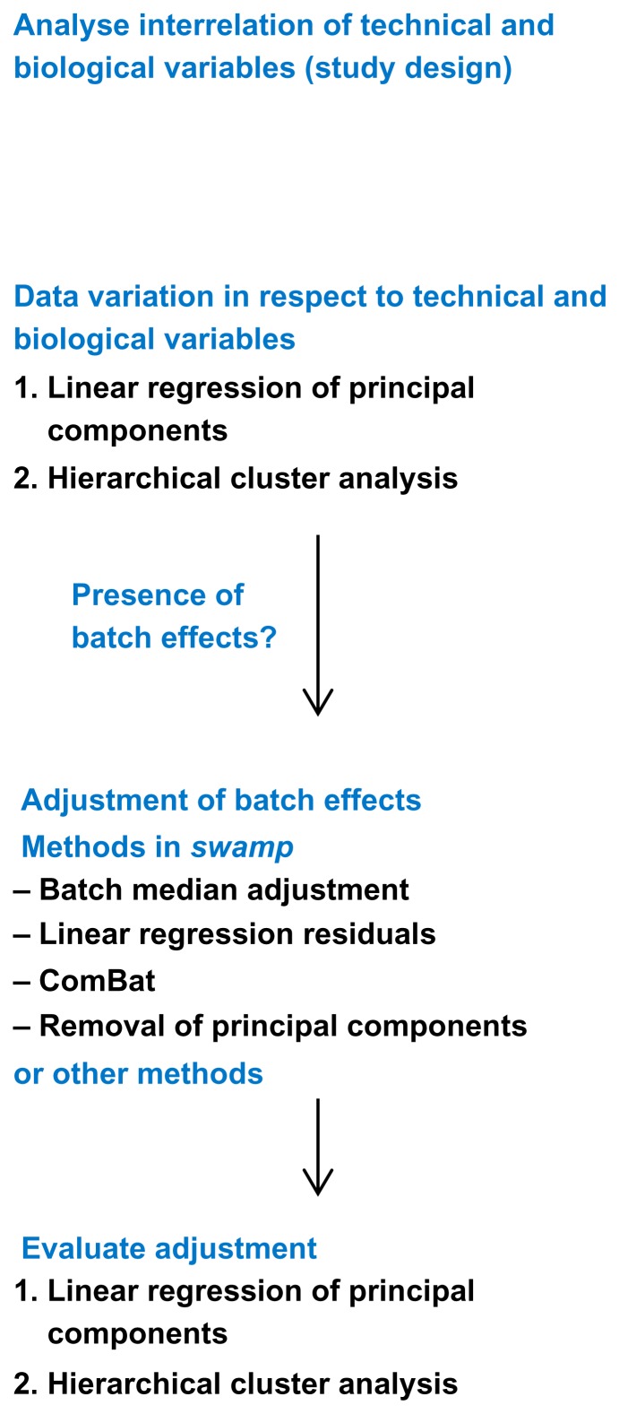
We have developed the R package swamp to provide algorithms and supportive plots for the analyses of high-throughput data in respect to sample annotations. The basic elements of the suggested framework presented in Figure 4 are:
Figure 4.
Framework to monitor technical variation.
Study design: Heatmap of the square matrix of log10P-values from pair-wise tests of sample annotations using Fisher/Chi-square test or linear models. Function: confounding.
Principal component analysis, using univariate linear regression models to determine the association between principal components and sample annotations. A heatmap of log10P-values or R2 values is plotted. Functions: prince, prince.plot.
Hierarchical clustering analysis and a quantification of batch effects across the dendrogram clusters using Fisher/Chi-square test or linear models for factors and numeric vectors respectively. Functions: hca.plot, hca.test.
We include two data correction methods that so far have not been implemented in R packages: The function kill.pc removes principal components from the data, as described by Alter et al.13 Principal components are deleted from the data by setting the corresponding singular values to zero and recalculating the data matrix. The function adjust.linearmodel uses the lm() function to obtain for each probe the residuals of a linear regression model with the technical variable as regressor. The adjust.linearmodel function makes it possible to correct the data for continuous technical variables. Furthermore we implemented the popular Com-Bat algorithm,7 taken from the webpage http://www.bu.edu/jlab/wp-assets/ComBat, in the function combat. The functions batchadjust.ref and bachadjust.zero perform simple median-centering of each probe and batch.
Additional batch correction methods, which may be more appropriate for certain data types, can be found in dedicated R packages for dwd,14 poe,15 sva,16 isva,17 pls-sva,18 and xpn.12
Data processing
For RNAseq data, we downloaded level3 RNAseqv2 data from the Cancer Genome Atlas (TCGA) data portal. We used the files that contain ‘reads per kilo-base per million mapped reads’ (RPKM) values for each gene. There is currently no standard processing pipeline of RPKM values. In the case of colon cancer, we used quantile-normalization as it removed substantial amounts of unexplained variation. For all RNAseq datasets from TCGA, we added an offset of 32, capped the data at 65,000, log2 transformed the data, and mean-centered the genes. This simple pre-processing method makes the data similar to the microarray gene expression format. It has been proposed that heteroscedastic RNAseq counts may influence downstream homoscedastic-based methods, such as principal component analysis.19 We therefore compared the simple pre-processing method with ‘variance stabilizing transformation’ (vst).19 However, we find that principal component analysis of TCGA data produces highly similar results for the simple pre-processing method and the vst-correction (Supplementary Fig. 1). In order to limit unnecessary data transformation, we did not continue to use vst-corrected data. For miRNAseq data, we downloaded level3 data from the TCGA data portal and performed the same data pre-processing (offset 32, cap 65,000, log2 transformation).
For methylation data we downloaded level2 data and calculated beta-values as M/(M+U), where M is methylated and U is unmethylated signal. For microarray gene expression data we used processed data from Leek et al.2 The batch variable in this dataset refers to date of hybridization, as derived from the headers of the cel files.
Availability and requirements
The R package swamp is freely available at CRAN. The package runs in R 2.15 or higher, and requires amap, gplots, and impute20 packages. A Windows software for swamp is freely available at http://co.bmc.lu.se/swamp/. The software is implemented in RGG language,21 and requires R 2.15 or higher and Java.
Results
Batch effects are found in a variety of datasets
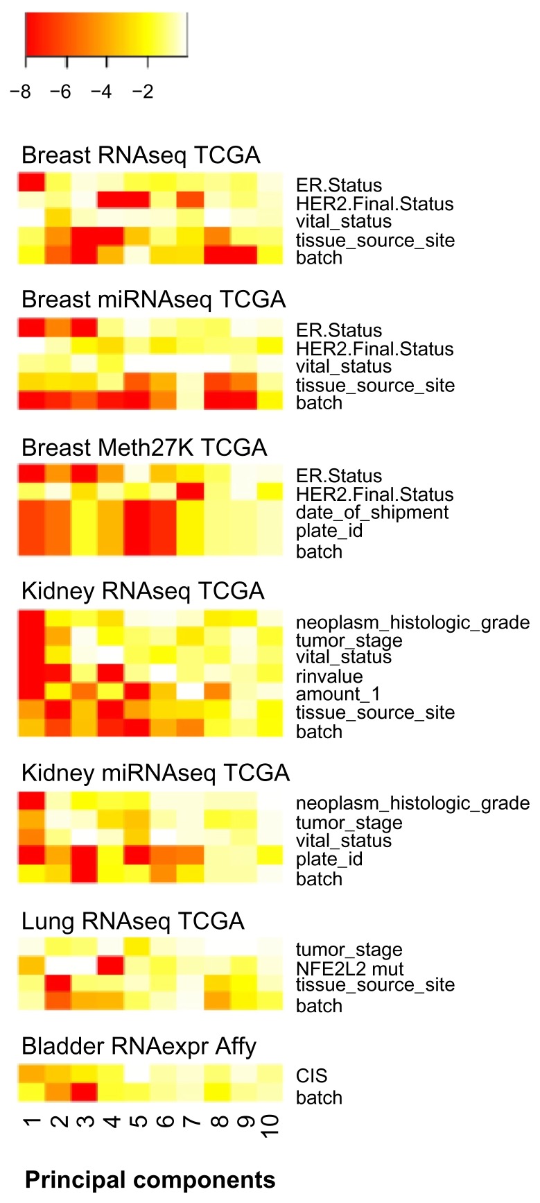
TCGA resource is remarkable as it reports technical variables in detail, notably by the MD Anderson Batch Effects Tool that implements the MBatch package. To visualize technical bias, such as batch effects, in high-throughput datasets, we introduce a plot which we call prince plot (Fig. 1). For the prince plot we perform a univariate linear regression of each principal component of a data matrix using the sample annotations as regressors. The heatmap of P-values shows the strength of associations of each sample annotation with the top principal components of a dataset. Biological variables are well associated to the top principal components, as shown in Figure 1, for several types of data, including RNAseq, miRNAseq, Methylation27K, and Affymetrix gene expression data. For instance, estrogen receptor status is strongly associated with top components of all three breast cancer datasets. In the kidney cancer RNAseq and miRNAseq data sets, histological grade and tumor stage are well associated with principal component 1. However, technical variables can also be associated to high-ranking principal components. In particular, the ‘batch’ annotations from TCGA data were associated to the top components in all types of investigated data (Fig. 1). The ‘batch’ variable is not further defined in the TCGA project; however, in most datasets correlates well with ‘tissue source site’ (hospital), ‘shipment date,’ and ‘plate-id’ variables. Notably, the ‘tissue source site’ variable can introduce slightly different bias when compared to the ‘batch’ variable, as observed in the breast cancer RNAseq data (Fig. 1). Sources of technical bias can also stem from continuous variables such as amount of DNA or RIN-value (RNA Integrity Number, ranges from 1 to 10) as observed in the kidney cancer RNAseq dataset. Furthermore, technical bias can occur in more than one principal component. For example, the batch variable of the lung cancer RNAseq data is associated with principal components 2, 3 and 4; and the strength of these associations differs across principal components. Biological variation may overlap technical variation and therefore can influence the same principal component. For example, principal component 2 of the bladder cancer expression data indicates that the technical ‘batch’ and the biological ‘CIS’ variables are interrelated. In summary, technical bias is present in all investigated high-throughput technologies, varies in effect size, and may overlap with biological variation in the data.
Figure 1.
Technical and biological variation in cancer high-throughput data.
Notes: The prince plots show the log10P-values from univariate linear regression of the top 10 principal components with sample annotations as regressors. The P-values are color-coded from red (P < 10−8) to white (P = 1). Sample annotations are named as in the TCGA biotab files or patient information tables of the respective TCGA portal publications.
Abbreviations: TCGA, The Cancer Genome Atlas; CIS, carcinoma in situ.
Monitoring of batch correction
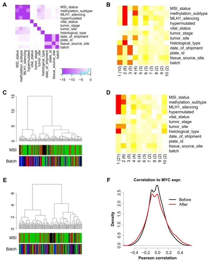
We took RNAseq data from TCGA’s colon cancer project generated using Illumina Hiseq2000 technology as an example.22 To make the analysis straightforward, we considered only the four largest sample batches. A plot of the interrelation of some important biological and technical variables revealed information on the study design of the TCGA colon project (Fig. 2A). The ‘batch’ variable overlaps with ‘date-of-shipment’ and ‘plate-id,’ as is the case for most TCGA projects. On the other hand, ‘batch’ is largely independent from biological variables such as ‘MSI status’ or ‘MLH1 silencing,’ indicating that each batch contains roughly the same biological composition. The prince plot shows that batch, together with other technical variables, confounds the first and the third component (Fig. 2B). The biological variables are highly associated with the second principal component and show moderate association with the fourth component. As biological and technical variables are associated to different sets of principal components, they contribute to uncorrelated variation patterns. No conclusions can be made a priori on the unexplained variance in the principal component analysis. For example, the variance in component 5 could be caused by either unknown technical or unknown biological processes. Batch effects have an immediate impact on unsupervised clustering analysis, with samples from the same batch clustering together (Fig. 2C). The two main colon cancer clusters are driven significantly by batch assignment (P = 2.5 × 10⁻⁶, Fisher test). We removed the first and third principal components from the dataset, as they are dominated by technical confounders and confirm the removal using a prince plot (Fig. 2D). This resulted in the batch variable being equally distributed across the two main clusters (Fig. 2E, P = 0.47). The TCGA publication concluded that MYC is a key regulator in colon cancer. We compared the associations of all genes on the platform to MYC expression, before and after correction (Fig. 2F). Before correction, 2879 genes were correlated to MYC at fdr = 0.05 while 4757 genes were after correction. Furthermore, there were 2406 genes before correction and 3924 genes after correction correlated to micro-satellite instability, respectively. It should be emphasized that successful batch correction can also decrease associations in supervised analysis. This is the case when the technical variable and the biological variable of interest are correlated. In such cases, the initial biological effect had been inflated by the batch effect.
Figure 2.
Adjustment of the RNAseq data from the TCGA colorectal cancer project.
Notes: The 4 largest batches of the colon cancer data are analyzed before and after data correction. (A) Confounding plot shows the association of sample annotations with P-values color-coded from purple (P < 10−8) to white (P = 1). (B) Prince plot before correction. Legend as in Figure 1, and percentage of variation for each principal component in brackets. (C) Hierarchical cluster analysis (HCA) using correlation as distance and ward algorithm as linkage method. MSI, microsatellite instability: green, stable microsatellites; red, MSI-low; black, MSI-high. (D) Prince plot after removal of principal components 1 and 3. (E) HCA after correction. (F) Correlation of the expression of all genes on the platform to MYC expression before (black) and after (green) correction.
Monitoring of dataset merging
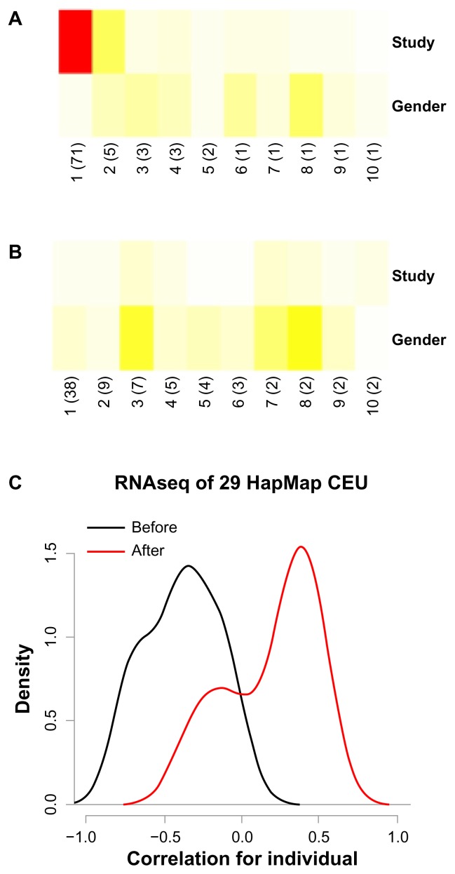
In another example, two RNAseq datasets taken from the ReCount database were assessed.23 Here, two labs used independently generated B-lymphocyte cell lines from the same 29 HapMap samples. A large association of the study variable was found with the first principal component of the merged data (Fig. 3A), and corrected the data by setting the median of each probe to be the same in both studies. Gender remained associated to the data after correction (Fig. 3B). The gender association is weak, however, as it relies on only 3 Y-chromosome genes, expressed in males. The highest expressed gene, RPS4Y1, shows increased male-specific expression after study correction (before: P = 6 × 10⁻⁹; after: P = 3 × 10⁻¹⁵). For a single HapMap individual, RNAseq data across the two studies should be similar. Before study correction sample pairs, however, are anti-correlated. This is due to the strong effect of the study variable in combination with low biological variation, as all cell lines are derived from lymphocytic cells of healthy individuals. Mean correlation values of HapMap cell line pairs increase after study correction, from −0.38 to 0.29 (Fig. 3C).
Figure 3.
Merging of two HapMap RNAseq datasets.
Notes: RNAseq data of 29 HapMap cell lines from two independent studies. (A) Prince plot before study correction and (B) after correction. (C) Density plot of correlations of HapMap cell line pairs before (black) and after (red) study correction.
Discussion
We find that large RNAseq datasets, such as those generated by the TCGA,22,24–26 can be burdened with technical variation and that this bias distorts downstream analysis. For expression microarray data, it has been shown that standard normalization pipelines may perform poorly to remove batch effects.2 In the colon RNA-seq dataset from TCGA, we applied quantile-normalization to RPKM values, thereby removing unexplained variances. However, batch effects remained after quantile-normalization. Applying a vst, as suggested for RNAseq data,19 did not make a notable impact on the TCGA datasets. For sequencing technologies, it may be possible that platform-tailored alignment and pre-processing algorithms can reduce batch effects, and we would argue that the prince plot is an adequate tool to monitor improvements.
The high prevalence of batch effects has important implications on study design. As it is unclear how to avoid batch effects, it may be wise to consider a study design that allows for repairing batch effects. In the worst case, biological variables and technical variables are highly correlated, eg, Phenotype A was assayed preferentially on Date A, and Phenotype B was preferentially assayed on Date B. The removal of a batch effect in such a case will be problematic as it reduces the biological variation in the data. To be able to correct for batch effects, each batch should be a good representation of the overall cohort. If there remains a risk that a strong biological variable is unknown, randomization of samples across batches may be a good strategy. A sufficiently large number of samples per batch are needed to statistically secure biological independence of batches. When the data is a compendium of small batches, batch correction is likely to shift biological variation, and hence outweighs the benefits. Unfortunately, many TCGA batches show biological selection and are small-sized, which makes it problematic to provide batch-corrected data.
To control batch effects, we propose a simple framework (Fig. 4). During the experiment all possible sources of technical variation are recorded and put into relation with biological annotations. The data is then screened by a prince plot and hierarchical clustering analysis. This may lead to detection of batch effects and subsequent batch correction efforts. If the correction algorithms provided by the swamp package are not suitable for a certain dataset, we encourage the use of an alternative algorithm from the literature. The choice of batch correction algorithm is likely to be dependent on study design,12 pre-processing steps, sample type, and platform. Regardless of the chosen algorithm, it is important to monitor the success of batch correction. Therefore, the outcome of data manipulation is controlled again by a prince plot/HCA. The elements of this framework are implemented in the R package swamp.
Conclusions
In summary, we find that high-throughput datasets which result in continuous measurements are potentially subject to technical biases. In such data, we argue that it is essential to monitor batch effects, eg, using the prince plot. Furthermore, we recommend a study design that keeps technical and biological variables independent, to be able to take rescue actions. To increase transparency and reproducibility of scientific findings, data submissions to public repositories should include technical variables.
Supplementary Figure
Simple data processing vs. variance stabilizing transformation.
Notes: The prince plots show the log10P-values from univariate linear regression of the top 10 principal components with sample annotations as regressors. The P-values are color-coded from red (P < 10−8) to white (P = 1). For sample annotations see Figure 1.
Footnotes
Author Contributions
ML has conceived the study, scripted the R package, analyzed the data and wrote the manuscript. IV and AK have developed the GUI software. MR and GJ have assisted in data analyses. MH conceived and supervised the study and wrote the manuscript. All authors read and approved the final manuscript.
Competing Interests
Author(s) disclose no potential conflicts of interest.
Disclosures and Ethics
As a requirement of publication the authors have provided signed confirmation of their compliance with ethical and legal obligations including but not limited to compliance with ICMJE authorship and competing interests guidelines, that the article is neither under consideration for publication nor published elsewhere, of their compliance with legal and ethical guidelines concerning human and animal research participants (if applicable), and that permission has been obtained for reproduction of any copyrighted material. This article was subject to blind, independent, expert peer review. The reviewers reported no competing interests.
Funding
This work was supported by the Swedish Cancer Society, the Swedish Research Council and the Nilsson Cancer Foundation.
References
- 1.Lazar C, Meganck S, Taminau J, et al. Batch effect removal methods for microarray gene expression data integration: a survey. Brief Bioinformatics. 2013;14(4):469–90. doi: 10.1093/bib/bbs037. [DOI] [PubMed] [Google Scholar]
- 2.Leek JT, Scharpf RB, Bravo HC, et al. Tackling the widespread and critical impact of batch effects in high-throughput data. Nat Rev Genet. 2010;11(10):733–9. doi: 10.1038/nrg2825. [DOI] [PMC free article] [PubMed] [Google Scholar]
- 3.Teschendorff AE, Menon U, Gentry-Maharaj A, et al. An epigenetic signature in peripheral blood predicts active ovarian cancer. PLoS ONE. 2009;4(12):e8274. doi: 10.1371/journal.pone.0008274. [DOI] [PMC free article] [PubMed] [Google Scholar]
- 4.Scharpf RB, Ruczinski I, Carvalho B, Doan B, Chakravarti A, Irizarry RA. A multilevel model to address batch effects in copy number estimation using SNP arrays. Biostatistics. 2011;12(1):33–50. doi: 10.1093/biostatistics/kxq043. [DOI] [PMC free article] [PubMed] [Google Scholar]
- 5.Taminau J, Meganck S, Lazar C, et al. Unlocking the potential of publicly available microarray data using inSilicoDb and inSilicoMerging R/Bioconductor packages. BMC Bioinformatics. 2012;13:335. doi: 10.1186/1471-2105-13-335. [DOI] [PMC free article] [PubMed] [Google Scholar]
- 6.Boutros PC. LTR: Linear Cross-Platform Integration of Microarray Data. Cancer Inform. 2010;9:197–208. doi: 10.4137/cin.s5756. [DOI] [PMC free article] [PubMed] [Google Scholar]
- 7.Johnson WE, Li C, Rabinovic A. Adjusting batch effects in microarray expression data using empirical Bayes methods. Biostatistics. 2007;8(1):118–27. doi: 10.1093/biostatistics/kxj037. [DOI] [PubMed] [Google Scholar]
- 8.Benito M, Parker J, Du Q, et al. Adjustment of systematic microarray data biases. Bioinformatics. 2004;20(1):105–14. doi: 10.1093/bioinformatics/btg385. [DOI] [PubMed] [Google Scholar]
- 9.Leek JT, Storey JD. Capturing heterogeneity in gene expression studies by surrogate variable analysis. PLoS Genet. 2007;3(9):1724–35. doi: 10.1371/journal.pgen.0030161. [DOI] [PMC free article] [PubMed] [Google Scholar]
- 10.Shabalin AA, Tjelmeland H, Fan C, Perou CM, Nobel AB. Merging two gene-expression studies via cross-platform normalization. Bioinformatics. 2008;24(9):1154–60. doi: 10.1093/bioinformatics/btn083. [DOI] [PubMed] [Google Scholar]
- 11.Chen C, Grennan K, Badner J, et al. Removing batch effects in analysis of expression microarray data: an evaluation of six batch adjustment methods. PLoS ONE. 2011;6(2):e17238. doi: 10.1371/journal.pone.0017238. [DOI] [PMC free article] [PubMed] [Google Scholar]
- 12.Rudy J, Valafar F. Empirical comparison of cross-platform normalization methods for gene expression data. BMC Bioinformatics. 2011;12:467. doi: 10.1186/1471-2105-12-467. [DOI] [PMC free article] [PubMed] [Google Scholar]
- 13.Alter O, Brown PO, Botstein D. Singular value decomposition for genome-wide expression data processing and modeling. Proc Natl Acad Sci U S A. 2000;97(18):10101–6. doi: 10.1073/pnas.97.18.10101. [DOI] [PMC free article] [PubMed] [Google Scholar]
- 14.Huang H, Lu X, Liu Y, Haaland P, Marron JS. R/DWD: distance-weighted discrimination for classification, visualization and batch adjustment. Bioinformatics. 2012;28(8):1182–3. doi: 10.1093/bioinformatics/bts096. [DOI] [PMC free article] [PubMed] [Google Scholar]
- 15.Scharpf R, Garrett ES, Hu J, Parmigiani G. Statistical modeling and visualization of molecular profiles in cancer. BioTechniques. 2003;(Suppl):22–9. [PubMed] [Google Scholar]
- 16.Leek JT, Johnson WE, Parker HS, Jaffe AE, Storey JD. The sva package for removing batch effects and other unwanted variation in high-throughput experiments. Bioinformatics. 2012;28(6):882–3. doi: 10.1093/bioinformatics/bts034. [DOI] [PMC free article] [PubMed] [Google Scholar]
- 17.Teschendorff AE, Zhuang J, Widschwendter M. Independent surrogate variable analysis to deconvolve confounding factors in large-scale microarray profiling studies. Bioinformatics. 2011;27(11):1496–505. doi: 10.1093/bioinformatics/btr171. [DOI] [PubMed] [Google Scholar]
- 18.Chakraborty S, Datta S, Datta S. Surrogate variable analysis using partial least squares (SVA-PLS) in gene expression studies. Bioinformatics. 2012;28(6):799–806. doi: 10.1093/bioinformatics/bts022. [DOI] [PubMed] [Google Scholar]
- 19.Anders S, Huber W. Differential expression analysis for sequence count data. Genome Biol. 2010;11(10):R106. doi: 10.1186/gb-2010-11-10-r106. [DOI] [PMC free article] [PubMed] [Google Scholar]
- 20.Troyanskaya O, Cantor M, Sherlock G, et al. Missing value estimation methods for DNA microarrays. Bioinformatics. 2001;17(6):520–5. doi: 10.1093/bioinformatics/17.6.520. [DOI] [PubMed] [Google Scholar]
- 21.Visne I, Dilaveroglu E, Vierlinger K, et al. RGG: a general GUI Framework for R scripts. BMC Bioinformatics. 2009;10:74. doi: 10.1186/1471-2105-10-74. [DOI] [PMC free article] [PubMed] [Google Scholar]
- 22.Cancer Genome Atlas Research Network. Comprehensive molecular characterization of human colon and rectal cancer. Nature. 2012;487(7407):330–7. doi: 10.1038/nature11252. [DOI] [PMC free article] [PubMed] [Google Scholar]
- 23.Frazee AC, Langmead B, Leek JT. ReCount: a multi-experiment resource of analysis-ready RNA-seq gene count datasets. BMC Bioinformatics. 2011;12:449. doi: 10.1186/1471-2105-12-449. [DOI] [PMC free article] [PubMed] [Google Scholar]
- 24.Cancer Genome Atlas Research Network. Comprehensive molecular portraits of human breast tumours. Nature. 2012;490(7418):61–70. doi: 10.1038/nature11412. [DOI] [PMC free article] [PubMed] [Google Scholar]
- 25.Cancer Genome Atlas Research Network. Comprehensive genomic characterization of squamous cell lung cancers. Nature. 2012;489(7417):519–25. doi: 10.1038/nature11404. [DOI] [PMC free article] [PubMed] [Google Scholar]
- 26.Cancer Genome Atlas Research Network. Comprehensive molecular characterization of clear cell renal cell carcinoma. Nature. 2013;499(7456):43–9. doi: 10.1038/nature12222. [DOI] [PMC free article] [PubMed] [Google Scholar]
Associated Data
This section collects any data citations, data availability statements, or supplementary materials included in this article.
Supplementary Materials
Simple data processing vs. variance stabilizing transformation.
Notes: The prince plots show the log10P-values from univariate linear regression of the top 10 principal components with sample annotations as regressors. The P-values are color-coded from red (P < 10−8) to white (P = 1). For sample annotations see Figure 1.


